Optimal H¹-Norm Estimation of Nonconforming FEM for Time-Fractional Diffusion Equation on Anisotropic Meshes

Abstract

In this paper, based on the $L2$-$1_{\sigma }$ scheme and nonconforming $E{Q}_1^{rot}$ finite element method (FEM), a numerical approximation is presented for a class of two-dimensional time-fractional diffusion equations involving variable coefficients. A novel and detailed analysis of the equations with an initial singularity is described on anisotropic meshes. The fully discrete scheme is shown to be unconditionally stable, and optimal second-order accuracy for convergence and superconvergence can be achieved in both time and space directions. Finally, the obtained numerical results are compared with the theoretical analysis, which verifies the accuracy of the proposed method.

1. Introduction

The development of fractional calculus has marked a significant impact on partial differential equations involving fractional differential operators. Especially in recent years, the applications of fractional partial differential equations have emerged in viscoelastic (See [1,2]), electromagnetic (See [3,4]), fluid dynamics (See [5]), control theory (See [6]), image processing (See [7]), ion-channel gating dynamics in some proteins (See [8]), airfoil theory, tumor development (See [9]), etc. For example, several fractional models have been successfully used to describe physical phenomena (See [10]). Furthermore, sufficient conditions for the existence of solutions to fractional differential equations involving Caputo derivatives were discussed in [11]. The analytical solutions of fractional differential equations are difficult to calculate using mathematical or analytical methods due to the complexity of fractional differential equations. Therefore, it is essential to develop efficient numerical methods and conduct rigorous numerical analysis for fractional partial differential equations, especially the time-fractional diffusion equation (See [12,13]), which is very useful in modeling physical and biological systems.

Some efforts have been devoted to time-fractional diffusion equations. Using the first-order finite difference scheme in both time and space directions, Liu et al. derived some stability conditions for the time-fractional diffusion equation in [14]. Lin et al. applied the backward differentiation and collocation method to numerically solve the time-fractional diffusion problem over finite fields, spatial exponential convergence and temporal $2-\alpha$ order accuracy can be obtained, where $\alpha (0<\alpha <1)$ represents the order of the fractional derivative (See [15]). Two finite difference/element methods were proposed in [16] for time-fractional diffusion equations with Dirichlet boundary conditions. Based on the spatial mixed FEM and the classical $L1$ time step method, Zhao et al. established an unconditionally stable fully discrete approximation scheme for the time-fractional diffusion equation, and the global superconvergence result was derived (See [17]). By constructing a higher-order $L2$-1${}_{\sigma }$ scheme for the Caputo fractional derivative, [18] investigated the time-fractional variable coefficient diffusion equation and demonstrated the stability and convergence in the $L^2$-norm. Using the $L2$-1${}_{\sigma }$ format and an unconditionally stable difference scheme, Gao et al. numerically solved the multi-term and distributed-order time-fractional diffusion equations (See [19]). Ref. [20] proposed a linear quasi-compact finite difference scheme for semi-linear space-fractional diffusion equations with time delays. And the time-space fractional nonlinear diffusion equation received attention in [21,22].

Furthermore, Refs. [23,24] discussed the regularity of the solution to the time-fractional diffusion problem and suggested that a key consideration in solving the time-fractional diffusion problem is the nonsmoothness of the solution at the initial time. As a result, some researchers mainly focus on initial singularity. Jin et al. revisited the $L1$ format error analysis and established $O\left(\tau \right)$ order convergence results for smooth and nonsmooth initial data (See [25]). Using graded meshes is one way to deal with initial singularity (See [26]). By combining the $L1$ scheme and spatial standard finite difference method on graded meshes, Ref. [27] presented a new analysis of stability and convergence for the time-fractional reaction-diffusion problem. Through complementary discrete convolution kernels, the global consistency error of fractional derivatives on graded meshes was deduced in [28], and the convergence analysis of the $L1$-FEM for the time-fractional reaction-diffusion equation was provided. The results in [27,28] showed that optimal $2-\alpha$ order convergence can be achieved by choosing the suitable temporal mesh parameter. In addition, combining the $L2$-$1_{\sigma }$ scheme and the bilinear FEM, the $L^2$-norm error analysis of the time-fractional diffusion equation was described in [29]. With the aid of the time-space splitting technique, [30] established $H^1$-norm error estimates of two finite difference methods for the time-fractional reaction-diffusion problem on graded meshes. Refs. [31,32] presented fully discrete schemes of $L2$-$1_{\sigma }$ FE/spectral method on graded meshes for the time-fractional reaction-diffusion equations, and stability and convergence were deduced.

In the above analysis of smooth or nonsmooth data, the researchers were committed to developing a more efficient and accurate method. It is well known that superconvergence is an effective method for improving the accuracy of FE approximation. For example, Ref. [33] provided $L^{\infty }\left(H^1\right)$ error estimates and superconvergence results for the multi-term time-fractional diffusion problem utilizing the $L1$-FEM on graded meshes. Moreover, by combining the $L2$-$1_{\sigma }$ scheme on graded meshes and the nonconforming Wilson FEM, the superconvergence analysis of the time-fractional diffusion equation was demonstrated in [34]. However, it appears that the temporal accuracy in the analysis of [34] is reduced by $r\alpha /2$. As a result, we re-analyzed the two-dimensional time fractional diffusion equation with variable coefficients to achieve optimal accuracy. The nonconforming FEM is an economical and flexible numerical method and is popular for its better convergence behavior. To the best of our knowledge, there has been limited research on the optimal superconvergence analysis of the two-dimensional time-fractional diffusion equation without sacrificing temporal accuracy. Therefore, the goal of this paper is to perform the optimal $H^1$-norm error estimation and superconvergence analysis of the $L2$-$1_{\sigma }$ nonconforming $E{Q}_1^{rot}$ FEM for the time-fractional variable coefficient diffusion equation.

The two-dimensional time-fractional variable coefficient diffusion equation can be described as:

$${\displaystyle D_t^{\alpha }u(\mathit{x},t)-\nabla ·(J\left(\mathit{x}\right)\nabla u)=f(\mathit{x},t),(\mathit{x},t)\in \Omega \times (0,T]}$$

(1)

with a Dirichlet boundary condition

$$u(\mathit{x},t)=0,(\mathit{x},t)\in \partial \Omega \times (0,T]$$

and a initial condition

$$u(\mathit{x},0)=u^0\left(\mathit{x}\right),\mathit{x}\in \Omega ,$$

$\Omega \subset R^2$ is a rectangular domain with a boundary $\partial \Omega$. The divergence operator and the gradient operator are represented by the symbol $\nabla ·$ and the symbol ∇, respectively. $J\left(\mathit{x}\right)$ is a smooth, bounded diffusion coefficient that satisfies $0<J_1^{-1}\le J\left(\mathit{x}\right)\le J_1,$ where $J_1$ is a positive constant. $u^0\left(\mathit{x}\right)$ and $f(\mathit{x},t)$ are the initial value function and the right-side source term, respectively. The operator $D_t^{\alpha }$ is the $\alpha$-order left-sided Caputo fractional derivative with respect to t. For $\alpha \in (0,1)$, $D_t^{\alpha }u(\mathit{x},t)$ is defined as

$${\displaystyle D_t^{\alpha }u(\mathit{x},t)=\frac{1}{\Gamma (1-\alpha )}{\int }_0^t\frac{\partial u(\mathit{x},\eta )}{\partial \eta }\frac{d\eta }{{(t-\eta )}^{\alpha }},}$$

where $\Gamma (·)$ is the Gamma function.

In this paper, it is assumed that there is a solution $u(\mathit{x},t)$ to Equation (1) such that $|{\partial }_t^{l}u(\mathit{x},t)|\lesssim 1+t^{\alpha -l}(l=0,1,2,3)$. It should be noted that this is a reasonable assumption satisfied by the typical problem solution (1). In addition, [24] illustrated that if the solution $u(\mathit{x},t)$ of Equation (1) is not as singular as assumed, that is, $|{\partial }_t^{l}u(\mathit{x},t)|\lesssim 1+t^{\gamma -l}$$(l=0,1,2,3)$ for $\gamma >\alpha$. Then the initial condition $u^0$ will be uniquely defined by the other data of the equation, which is obviously restrictive.

The rest of this paper is organized as follows. In Section 2, the $L2$-$1_{\sigma }$ scheme and some lemmas are introduced. Section 3 is devoted to the spatial discretization of the nonconforming $E{Q}_1^{rot}$ FEM. The fully discrete scheme and unconditional stability are discussed in Section 4. In Section 5, the $L^2$-norm error estimate and the suboptimal $H^1$-norm estimate are derived. The optimal $H^1$-norm estimation is supplemented in Section 6. In Section 7, the interpolation postprocessing technique is introduced and the $H^1$-norm global superconvergence result is presented. Section 8 implements numerical experiments to demonstrate the accuracy of our theoretical analysis. Finally, a brief conclusion completes our work.

2. $L2$-$1_{\sigma }$ Approximation on Graded Meshes

Notations. $a\lesssim b$ denotes $a⩽Cb$. The existence of $a\lesssim b$ and $b\lesssim a$ is described by $a\backsimeq b$. C is a positive constant and independent of mesh parameters, it can take various values in different locations.

2.1. Direct Error Analysis for $L2$-$1_{\sigma }$ Time-Stepping Scheme

Select the graded meshes ${\displaystyle t_n=T{(n/N)}^r(r\ge 1)}$ at $n=0,\dots ,N$, and N is a positive integer. Then the time step ${\tau }_n=t_n-t_{n-1}$ and $t_{n+\sigma }=t_n+\sigma {\tau }_{n+1}(0\le \sigma \le 1)$. For the function $v\left(t\right)$ defined on $[0,T]$, we denote

$${\displaystyle v^n=v\left(t_n\right),v^{n+\sigma }=v\left(t_{n+\sigma }\right),v^{\overline{n}}=\sigma v^{n+1}+(1-\sigma )v^n\mathrm{and}{\delta }_t{v}^n=(v^{n+1}-v^n)/{\tau }_{n+1}.}$$

The properties of the graded meshes ${\left\{t_n\right\}}_{n=0}^N$ are described in Lemma 1 below.

Lemma 1.

For the graded meshes ${\left\{t_n\right\}}_{n=0}^N$, we have

$$t_n\ge \frac{t_{n+1}}{2^r}and{\tau }_n\backsimeq T^{\frac{1}{r}}{N}^{-1}{t}_n^{1-\frac{1}{r}}.$$

Proof. 

From the definition of ${\left\{t_n\right\}}_{n=0}^N$, we can deduce

$${\displaystyle \frac{t_n}{t_{n+1}}={\left(\frac{n}{n+1}\right)}^r\ge \frac{1}{2^r}.}$$

That is, for ${\displaystyle n=1,2\dots ,N-1,t_n\ge \frac{t_{n+1}}{2^r}}$.

Furthermore, we derive the time step

$${\displaystyle {\tau }_n=t_n-t_{n-1}=T\frac{n^r-{(n-1)}^r}{N^r}=T^{1-\frac{1}{r}}{\left(\frac{n}{N}\right)}^{r-1}{T}^{\frac{1}{r}}{\left(\frac{n}{N}\right)}^{1-r}\frac{n^r-{(n-1)}^r}{N^r}=t_n^{1-\frac{1}{r}}{T}^{\frac{1}{r}}{N}^{-1}{j}^{1-r}(j^r-{(j-1)}^r).}$$

$j^{1-r}(j^r-{(j-1)}^r)$ can be discussed in two situations. For $j=1$, the equation $j^{1-r}(j^r-{(j-1)}^r)=1$ is established.

Using the Cauchy mean value theorem, we have

$${\displaystyle j^{1-r}(j^r-{(j-1)}^r)=\frac{j^r-{(j-1)}^r}{j^{r-1}}=\frac{r{(j-{\theta }_j)}^{r-1}}{j^{r-1}}=r{\left(\frac{j-{\theta }_j}{j}\right)}^{r-1}=r{\left(1-\frac{{\theta }_j}{j}\right)}^{r-1}\mathrm{for}j\ge 2,{\theta }_j\in (0,1).}$$

It is not difficult to obtain ${\displaystyle {\tau }_n\backsimeq T^{\frac{1}{r}}{N}^{-1}{t}_n^{1-\frac{1}{r}}}$ for $n=1,2\dots ,N$ with the help of

$${\displaystyle r{\left(\frac{1}{2}\right)}^{r-1}\le r{\left(1-\frac{1}{2}\right)}^{r-1}\le r{\left(1-\frac{{\theta }_j}{j}\right)}^{r-1}\le r.}$$

□

The $L2$-$1_{\sigma }$ time step scheme proposed in [18] is used in this paper to approximate the Caputo fractional derivative $D_t^{\alpha }{v}^{n+\sigma }$:

$$D_t^{\alpha }{v}^{n+\sigma }\approx {\delta }_t^{\alpha }{v}^{n+\sigma }=\sum _{k=0}^n{A}_{n-k}^{n+1}(v^{k+1}-v^k),n=0,\dots N-1.$$

Lemma 2

([18]). For a function $v(\mathit{x},t)$ and the $L2$-$1_{\sigma }$ approximation ${\delta }_t^{\alpha }{v}^{n+\sigma }$ on the graded meshes ${\left\{t_n\right\}}_{n=0}^N,$ we have

$$2(v^{\overline{n}},{\delta }_t^{\alpha }{v}^{n+\sigma })\ge {\delta }_t^{\alpha }{\parallel v^{n+\sigma }\parallel }^2,n=0,\dots ,N-1.$$

In this article, $(·,·)$ is the inner product in the space $L^2(\Omega )$, and $\parallel ·\parallel$ denotes the $L^2$-norm. For each $q\in \mathbb{N},\mathbb{N}=\{1,2,3,\dots \},$ the symbol $H^q(\Omega )$ represents the standard Sobolev space with the corresponding norm ${\parallel ·\parallel }_q$ and semi-norm ${|·|}_q$. $L^{\infty }(0,T;H^m(\Omega ))$ expresses the space of the measurable function $v:(0,T)\to H^m(\Omega )$, and v satisfies ${\displaystyle {\parallel v\parallel }_{L^{\infty }\left(H^m\right)}=\mathrm{ess}\underset{0\le t\le T}{sup}{\parallel v\left(t\right)\parallel }_m<+\infty }$.

Lemma 3

([32]). Assume that $1-\alpha /2\le \sigma \le 1$. For a function $v\left(t\right)$ defined on the graded meshes ${\left\{t_k\right\}}_{k=0}^N$, we have

$$|v^{n+1}|\le |v^0|+\Gamma (1-\alpha )\underset{k=0,\dots ,n}{max}\{t_{k+\sigma }^{\alpha }{\delta }_t^{\alpha }|v^{k+\sigma }\left|\right\},n=0,\dots ,N-1.$$

Remark 1.

Similar to the derivation of Lemma 3 in [32], replacing $|·|$ with $\parallel ·\parallel$ and the conclusion is still valid.

Lemma 4.

For a function $v(\mathit{x},t)$ defined on the graded meshes ${\left\{t_n\right\}}_{n=0}^N$, assuming $\sigma =1-\alpha /2$ and $\parallel {\partial }_t^l{v(\mathit{x},t)\parallel }_{q_1}\lesssim 1+t^{\alpha -l}(q_1=0,1)\mathrm{for}l=0,1,2,3,$ we have

$$t_{n+\sigma }^{\alpha }{\parallel {\delta }_t^{\alpha }{v}^{n+\sigma }-D_t^{\alpha }{v}^{n+\sigma }\parallel }_{q_1}\lesssim N^{-min\{r\alpha ,3-\alpha \}},n=0,\dots ,N-1.$$

Proof. 

We know from the result in [32] that $t_{n+\sigma }^{\alpha }|{\delta }_t^{\alpha }{v}^{n+\sigma }-D_t^{\alpha }{v}^{n+\sigma }|\lesssim N^{-min\{r\alpha ,3-\alpha \}}$ is true for the function $v\left(t\right)$ that satisfy $v\left(t\right)\in C\left([0,T]\right)\cap C^3\left((0,T]\right)$ and $|v^{\left(l\right)}\left(t\right)|\lesssim 1+t^{\alpha -l}$$(l=0,1,2,3)$.

Furthermore, for the function $v(\mathit{x},t)$, if $\parallel {\partial }_t^l{v(\mathit{x},t)\parallel }_{q_1}\lesssim 1+t^{\alpha -l}(q_1=0,1)$ for $l=0,1,2,3,$ the conclusion presented in Lemma 4 is not difficult to deduce. □

Lemma 5.

Assume the function $v(\mathit{x},t)\in L^{\infty }(0,T;H_0^1(\Omega )\bigcap H^{2+q_2}(\Omega ))$ and $\parallel {\partial }_t^l{v(\mathit{x},t)\parallel }_{2+q_2}\lesssim 1+t^{\alpha -l}(q_2=0,1,2)forl=0,1,2,3,$ we have

$$t_{n+\sigma }^{\alpha }{\parallel \nabla ·(J\left(\mathit{x}\right)\nabla (v^{\overline{n}}-v^{n+\sigma }))\parallel }_{q_2}\lesssim N^{-min\{r\alpha ,2\}}.$$

Proof. 

Using Taylor’s theorem, it is easy to derive

$$|v^{\overline{n}}-v^{n+\sigma }|\le \frac{1}{8}{\tau }_{n+1}^2\underset{t\in (t_n,t_{n+1})}{max}\left|v^{″}\left(t\right)\right|\mathrm{for}v\left(t\right)\in C^2\left((0,T]\right).$$

(2)

Using the result of (2), we have $t_{\sigma }^{\alpha }{\parallel \nabla ·(J\left(\mathit{x}\right)\nabla (v^{\overline{n}}-v^{n+\sigma }))\parallel }_{q_2}\lesssim t_1^{\alpha }\lesssim T^{\alpha }{N}^{-r\alpha }$ for $n=0$.

Combining Lemma 1, (2), and ${\displaystyle \parallel {\partial }_t^2{u(\mathit{x},t)\parallel }_{2+q_2}\lesssim t^{\alpha -2}}$ yields the following result

$${\displaystyle t_{n+\sigma }^{\alpha }{\parallel \nabla ·(J\left(\mathit{x}\right)\nabla (v^{\overline{n}}-v^{n+\sigma }))\parallel }_{q_2}\lesssim t_{n+\sigma }^{\alpha }{\tau }_{n+1}^2{t}_n^{\alpha -2}\lesssim t_{n+1}^{\alpha }{T}^{\frac{2}{r}}{N}^{-2}{t}_{n+1}^{2-\frac{2}{r}}{2}^{-r(\alpha -2)}{t}_{n+1}^{\alpha -2}\lesssim N^{-2}{t}_{n+1}^{2\alpha -\frac{2}{r}}\mathrm{for}n\ge 1.}$$

Furthermore,

$$t_{n+\sigma }^{\alpha }{\parallel \nabla ·(J\left(\mathit{x}\right)\nabla (v^{\overline{n}}-v^{n+\sigma }))\parallel }_{q_2}\lesssim \left\{\begin{array}{cc}{\displaystyle N^{-2},}\hfill & \mathrm{for}n=1,\dots ,N-1\mathrm{if}r\ge \frac{1}{\alpha },\hfill \\ {\displaystyle N^{-2}{t}_1^{2\alpha -\frac{2}{r}}\lesssim N^{-2}{N}^{-2r\alpha +2}\backsimeq N^{-2r\alpha },}\hfill & \mathrm{for}n=1,\dots ,N-1\mathrm{if}\frac{1}{\alpha }\ge r\ge 1\hfill \end{array}\right.$$

is established as a more precise result.

The preceding analysis indicates that obtaining the desired result is not difficult. □

2.2. Global Consistency Error Analysis for $L2$-$1_{\sigma }$ Time-Stepping Scheme

In this section, we introduce complementary discrete convolution kernels

$${\displaystyle p_0^{n+1}=\frac{1}{A_0^{n+1}},p_{n-j}^{n+1}=\frac{1}{A_0^{j+1}}\sum _{k=j+1}^n(A_{k-j-1}^{k+1}-A_{k-j}^{k+1})p_{n-k}^{n+1},0\le j\le n-1.}$$

And ${\displaystyle \sum _{j=k}^n{p}_{n-j}^{n+1}{A}_{j-k}^{j+1}\equiv 1}$ is established for the convolution kernels $p_{n-j}^{n+1}$.

In Lemma 6, we present the modified discrete fractional Grönwall inequality, which is based on the results in [30,31].

Lemma 6.

For given non-negative sequences ${\left\{{\omega }_{n-k}\right\}}_{k=0}^{N-1},{\left\{{\epsilon }^{k+1}\right\}}_{k=0}^{N-1}$ and ${\left\{{\zeta }^{k+1}\right\}}_{k=0}^{N-1}$, there is a constant ω independent of the time step, such that ${\sum }_{k=0}^{N-1}\left\{{\omega }_{n-k}\right\}\le \omega$. If the non-negative functions ${\left\{v^{k+1}\right\}}_{k=0}^{N-1}$ defined on graded meshes satisfy

$${\displaystyle \sum _{k=0}^n{A}_{n-k}^{n+1}\left({\left(v^{k+1}\right)}^2-{\left(v^k\right)}^2\right)\le \sum _{k=0}^n{\omega }_{n-k}{\left(v^{\overline{n}}\right)}^2+v^{\overline{n}}{\epsilon }^{n+1}+{\left({\zeta }^{n+1}\right)}^{2}for0\le n\le N-1,}$$

then

$${\displaystyle v^{n+1}\le 2E_{\alpha }\left(\frac{8}{3}\omega t_{n+1}^{\alpha }\right)\left(v^0+\underset{0\le k\le n}{max}\sum _{j=0}^k{p}_{k-j}^{k+1}{\epsilon }^{j+1}+\sqrt{4\Gamma (1-\alpha )/3}\underset{0\le k\le n}{max}{t}_{k+1}^{\alpha /2}{\zeta }^{k+1}\right)}$$

is true, where Mittag-Leffler function $E_{\alpha }\left(\varsigma \right)={\Sigma }_{k=0}^{\infty }{\varsigma }^k/\Gamma (1+k\varsigma )$.

The following Lemma 7 plays an important role in the error estimation in this paper.

Lemma 7.

Assuming $\parallel {\partial }_t^l{v(\mathit{x},t)\parallel }_{q_1}\lesssim 1+t^{\alpha -l}(q_1=2,3)$ holds for $l=0,1,2,3$, we can infer the result

$${\displaystyle \sum _{j=0}^n{p}_{n-j}^{n+1}{\parallel v^{\overline{n}}-v^{n+\sigma }\parallel }_{q_1}\lesssim {\tau }^{min\{\lambda \alpha ,2\}},0\le n\le N-1.}$$

(3)

In addition, if $\parallel {\partial }_t^l{v(\mathit{x},t)\parallel }_{q_2}\lesssim 1+t^{\alpha -l}(q_2=0,1)$ and $\sigma =1-\alpha /2$, we have

$${\displaystyle \sum _{j=0}^n{p}_{n-j}^{n+1}{\parallel {\delta }_t^{\alpha }{v}^{n+\sigma }-D_t^{\alpha }{v}^{n+\sigma }\parallel }_{q_2}\lesssim {\tau }^{min\{\lambda \alpha ,2\}},0\le n\le N-1.}$$

(4)

Proof. 

According to Lemmas 3.6 and 3.8 in [31], if $v\left(t\right)\in C^2\left((0,T]\right)$ and $|v^{″}\left(t\right)|\lesssim 1+t^{\alpha -2}$, then

$${\displaystyle \sum _{j=0}^n{p}_{n-j}^{n+1}|v^{\overline{n}}-v^{n+\sigma }|\lesssim {\tau }^{min\{\lambda \alpha ,2\}},0\le n\le N-1}$$

is established. Furthermore, if $\sigma =1-\alpha /2$, $v\left(t\right)\in C\left([0,T]\right)\cap C^3\left((0,T]\right)$, and $|v^{\left(l\right)}\left(t\right)|\lesssim 1+t^{\alpha -l}(l=0,1,2,3)$, we have

$${\displaystyle \sum _{j=0}^n{p}_{n-j}^{n+1}|{\delta }_t^{\alpha }{v}^{n+\sigma }-D_t^{\alpha }{v}^{n+\sigma }|\lesssim {\tau }^{min\{\lambda \alpha ,2\}},0\le n\le N-1.}$$

Inspired by the idea in [31], we assume $\parallel {\partial }_t^l{v(\mathit{x},t)\parallel }_{q_1}\lesssim 1+t^{\alpha -l}(q_1=2,3)$ and $\parallel {\partial }_t^l{v(\mathit{x},t)\parallel }_{q_2}\lesssim 1+t^{\alpha -l}(q_2=0,1)$ for $l=0,1,2,3$, the results (3) and (4) can be obtained, respectively. □

3. Nonconforming ${EQ}_1^{rot}$ FEM in Space

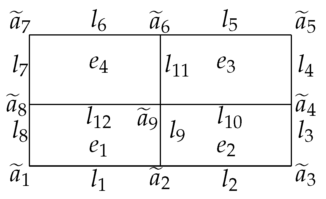
Let ${\Gamma }_h$ represent a family of anisotropic rectangular meshes on $\Omega$ with ${\displaystyle \overline{\Omega }={\cup }_{e\in {\Gamma }_h}e}$ that do not need to satisfy the regularity or quasi-uniformity assumptions. Assume that $O_e$ is the center of e for each $e\in {\Gamma }_h$. The four vertices of e are

$$A_1=(x_e-h_{x,e},y_e-h_{y,e}),A_2=(x_e+h_{x,e},y_e-h_{y,e}),A_3=(x_e+h_{x,e},y_e+h_{y,e}),\mathrm{and}{A}_4=(x_e-h_{x,e},y_e+h_{y,e}).$$

$O_e=(x_e,y_e)$, where $h_{x,e}$ and $h_{y,e}$ are the perpendicular distances between $O_e$ and two sides of e that are parallel to the two coordinate planes. Let $l_i=\overline{A_i{A}_{i+1}}(i=1,2,3,4.mod\left(4\right))$, $h_e=max\{h_{x,e},h_{y,e}\}$ and ${\displaystyle h=\underset{e\in {\Gamma }_h}{max}\left\{h_e\right\}.}$.

The FE space is defined as

$$V_h=\{v_h;v_h{|}_e\in \{1,x,y,x^2,y^2\},{\int }_F⟨v_h⟩ds=0,F\subset \partial e,\forall e\in {\Gamma }_h\},$$

where $⟨v_h⟩$ represents for the jump of $v_h$ across the edge F if F is an internal edge, and $⟨v_h⟩=v_h$ if F is a boundary edge.

Let $I_h:v\in H^1(\Omega )\to I_{h}v\in V_h$ be the associated interpolation operator satisfying

$$I_h{|}_e=I_e,{\int }_{l_i}(v-I_{e}v)ds=0,i=1,2,3,4,{\int }_e(v-I_{e}v)dxdy=0.$$

From [35,36], we can obtain the following estimation results of the interpolation operator $I_h$.

Lemma 8.

Assuming the function $v\in H_0^1(\Omega )\cap H^2(\Omega )$ on anisotropic meshes, we obtain

$$\parallel v-I_{h}v\parallel +h\parallel v-I_h{v\parallel }_1\lesssim h^2{\parallel v\parallel }_2$$

and

$$(\nabla (v-I_{h}v),\nabla v_h)=0,\forall v_h\in V_h.$$

The Ritz projection operator $R_h:H_0^1(\Omega )\to V_h$ is then defined, which satisfies $(J\left(\mathit{x}\right)\nabla (v-R_{h}v),\nabla v_h)=0,\forall v_h\in V_h.$ It is not difficult to conclude Lemma 9 from the results in Lemma 8, the definition of $R_h$, and the literature [37].

Lemma 9.

For any function $v\in H_0^1(\Omega )\cap H^2(\Omega )$, we have

$$\parallel R_{h}v-I_h{v\parallel }_1\lesssim h^2{\parallel v\parallel }_2$$

(5)

and

$$\parallel R_{h}v-v\parallel +h\parallel \nabla (R_{h}v-v)\parallel \lesssim h^2{\parallel v\parallel }_2.$$

(6)

Combining the results in Lemma 8 and 9 with the proof in [38], the expected result is given in Lemma 10.

Lemma 10.

If the function $v\in H_0^1(\Omega )\cap H^4(\Omega ),$ we have

$${\displaystyle \left|\sum _e{\int }_{\partial e}J\left(\mathit{x}\right)\frac{\partial v}{\partial \mathit{n}}{v}_{h}ds\right|\lesssim h^2{\parallel v\parallel }_4\parallel v_h\parallel ,\forall v_h\in V_h,}$$

where $|·|$ is the absolute value and $\mathit{n}$ is the unit normal vector on $\partial e$.

4. Stability in $L^2$-Norm and $H^1$-Norm

Combining the $L2$-$1_{\sigma }$ scheme and the nonconforming $E{Q}_1^{rot}$ FEM, the fully discrete scheme of (1) can be expressed as: find ${\left\{u_h^n\right\}}_{n=0}^N\in V_h$ such that

$$\left\{\begin{array}{cc}{\displaystyle \left({\delta }_t^{\alpha }{u}_h^{n+\sigma },v_h\right)+\left(J\left(\mathit{x}\right)\nabla {u_h}^{\overline{n}},\nabla v_h\right)=\left(f^{n+\sigma },v_h\right),}\hfill & \forall v_h\in V_h,\hfill \\ (u_h^0,v_h)=(u^0,v_h),\hfill & x\in \Omega .\hfill \end{array}\right.$$

(7)

The unconditional stability of the fully discrete scheme (7) is described in Theorem 1.

Theorem 1.

Let ${\left\{u_h^{n+1}\right\}}_{n=0}^{N-1}$ represent the solutions of (7). If the function $f\in L^{\infty }(0,T;L^2(\Omega ))$, we have

$${\displaystyle \parallel u_h^{n+1}{\parallel }^2\le \parallel u_h^0{\parallel }^2+\frac{\Gamma (1-\alpha )J_1{T}^{\alpha }}{2}\underset{k=0,\dots ,N-1}{max}{\parallel f^{k+\sigma }\parallel }^2}$$

and

$${\displaystyle \parallel \nabla u_h^{n+1}{\parallel }^2\le J_1^2\parallel \nabla u_h^0{\parallel }^2+\frac{\Gamma (1-\alpha )J_1{T}^{\alpha }}{2}\underset{k=0,\dots ,N-1}{max}{\parallel f^{k+\sigma }\parallel }^2.}$$

Proof. 

Taking $v_h=2{u_h}^{\overline{n}}$ in (7), (7) can be rewritten as

$$({\delta }_t^{\alpha }{u}_h^{n+\sigma },2{u_h}^{\overline{n}})+(J\left(\mathit{x}\right)\nabla {u_h}^{\overline{n}},2\nabla {u_h}^{\overline{n}})=(f^{n+\sigma },2{u_h}^{\overline{n}}).$$

(8)

From Lemma 2, we know that

$$({\delta }_t^{\alpha }{u}_h^{n+\sigma },2{u_h}^{\overline{n}})\ge {\delta }_t^{\alpha }{\parallel {u_h}^{n+\sigma }\parallel }^2.$$

(9)

With the aid of (9) and the condition $0<J_1^{-1}\le J\left(\mathit{x}\right)\le J_1$, applying the Cauchy-Schwartz inequality and Young’s inequality, (8) can be converted to

$$\begin{array}{c}{\displaystyle {\delta }_t^{\alpha }\parallel {u_h}^{n+\sigma }{\parallel }^2+\frac{2}{J_1}\parallel \nabla {u_h}^{\overline{n}}{\parallel }^2\le 2\parallel f^{n+\sigma }\parallel \parallel \nabla {u_h}^{\overline{n}}\parallel \le \frac{J_1}{2}\parallel f^{n+\sigma }{\parallel }^2+\frac{2}{J_1}{\parallel \nabla {u_h}^{\overline{n}}\parallel }^2,}\hfill \end{array}$$

that is ${\displaystyle {\delta }_t^{\alpha }\parallel {u_h}^{n+\sigma }{\parallel }^2\le \frac{J_1}{2}{\parallel f^{n+\sigma }\parallel }^2.}$ Remark 1 implies that

$$\begin{array}{cc}\parallel u_h^{n+1}{\parallel }^2\hfill & {\displaystyle \le \parallel u_h^0{\parallel }^2+\Gamma (1-\alpha )\underset{k=0,\dots ,n}{max}\{t_{k+\sigma }^{\alpha }{\delta }_t^{\alpha }\parallel {u_h}^{k+\sigma }{\parallel }^2\}}\hfill \\ \hfill & {\displaystyle \le \parallel u_h^0{\parallel }^2+\frac{\Gamma (1-\alpha )J_1{T}^{\alpha }}{2}\underset{k=0,\dots ,N-1}{max}{\parallel f^{k+\sigma }\parallel }^2.}\hfill \end{array}$$

Choosing $v_h=2{\delta }_t^{\alpha }{u_h}^{n+\sigma }$ in (7) to estimate $\parallel \nabla u_h^{n+1}\parallel$, we have

$$({\delta }_t^{\alpha }{u_h}^{n+\sigma },2{\delta }_t^{\alpha }{u_h}^{n+\sigma })+(J\left(\mathit{x}\right)\nabla {u_h}^{\overline{n}},2{\delta }_t^{\alpha }\nabla {u_h}^{n+\sigma })=(f^{n+\sigma },2{\delta }_t^{\alpha }{u_h}^{n+\sigma }).$$

(10)

Lemma 2 means that

$$(J\left(\mathit{x}\right)\nabla {u_h}^{\overline{n}},2{\delta }_t^{\alpha }\nabla {u_h}^{n+\sigma })\ge {\delta }_t^{\alpha }{\parallel \nabla \left(J^{\frac{1}{2}}\left(\mathit{x}\right){u_h}^{n+\sigma }\right)\parallel }^2.$$

(11)

Combining (11) with (10), we have

$$\begin{array}{c}{\displaystyle 2\parallel {\delta }_t^{\alpha }{u_h}^{n+\sigma }{\parallel }^2+{\delta }_t^{\alpha }\parallel \nabla \left(J^{\frac{1}{2}}\left(\mathit{x}\right){u_h}^{n+\sigma }\right){\parallel }^2\le 2\parallel f^{n+\sigma }\parallel \parallel {\delta }_t^{\alpha }{u_h}^{n+\sigma }\parallel \le \frac{1}{2}\parallel f^{n+\sigma }{\parallel }^2+2{\parallel {\delta }_t^{\alpha }{u_h}^{n+\sigma }\parallel }^2.}\hfill \end{array}$$

(12)

Then (12) can be rewritten as ${\displaystyle {\delta }_t^{\alpha }\parallel \nabla \left(J^{\frac{1}{2}}\left(\mathit{x}\right){u_h}^{n+\sigma }\right){\parallel }^2\le \frac{1}{2}{\parallel f^{n+\sigma }\parallel }^2.}$ Using Remark 1, we obtain that

$$\begin{array}{c}{\displaystyle \parallel \nabla \left(J^{\frac{1}{2}}\left(\mathit{x}\right)u_h^{n+1}\right){\parallel }^2\le \parallel \nabla \left(J^{\frac{1}{2}}\left(\mathit{x}\right)u_h^0\right){\parallel }^2+\frac{\Gamma (1-\alpha )T^{\alpha }}{2}\underset{k=0,\dots ,N-1}{max}{\parallel f^{k+\sigma }\parallel }^2.}\hfill \end{array}$$

(13)

Further, inequality (13) can be simplified to

$$\parallel \nabla u_h^{n+1}{\parallel }^2\le J_1^2\parallel \nabla u_h^0{\parallel }^2+\frac{\Gamma (1-\alpha )J_1{T}^{\alpha }}{2}\underset{k=0,\dots ,N-1}{max}{\parallel f^{k+\sigma }\parallel }^2.$$

□

5. Error Estimates in Optimal $L^2$-Norm and Suboptimal $H^1$-Norm

Subtracting (7) from (1) yields the error equation

$$\begin{array}{cc}\hfill & ({\delta }_t^{\alpha }(u^{n+\sigma }-{u_h}^{n+\sigma }),v_h)+(J\left(\mathit{x}\right)\nabla (u^{\overline{n}}-{u_h}^{\overline{n}}),\nabla v_h)\hfill \\ \hfill & {\displaystyle =-(R_1^{n+\sigma },v_h)+(\nabla ·(J\left(\mathit{x}\right)\nabla R_2^{n+\sigma }),v_h)+\sum _e{\int }_{\partial e}J\left(\mathit{x}\right)\frac{\partial u^{\overline{n}}}{\partial \mathit{n}}{v}_{h}ds-\sum _e{\int }_{\partial e}J\left(\mathit{x}\right)\frac{\partial R_2^{n+\sigma }}{\partial \mathit{n}}{v}_{h}ds,\forall v_h\in V_h,}\hfill \end{array}$$

where $R_1^{n+\sigma }=D_t^{\alpha }{u}^{n+\sigma }-{\delta }_t^{\alpha }{u}^{n+\sigma },R_2^{n+\sigma }=u^{n+\sigma }-u^{\overline{n}}.$

Denoting $u^n-{u_h}^n=u^n-R_h{u}^n+R_h{u}^n-u_h^n={\eta }^n+{\xi }^n,$ the error equation has the following form:

$$\begin{array}{cc}\left({\delta }_t^{\alpha }{\xi }^{n+\sigma },v_h\right)+\left(J\left(\mathit{x}\right)\nabla {\xi }^{\overline{n}},\nabla v_h\right)\hfill & =-\left({\delta }_t^{\alpha }{\eta }^{n+\sigma },v_h\right)-\left(J\left(\mathit{x}\right)\nabla {\eta }^{\overline{n}},\nabla v_h\right)-\left(R_1^{n+\sigma },v_h\right)+\left(\nabla ·(J\left(\mathit{x}\right)\nabla R_2^{n+\sigma }),v_h\right)\hfill \\ \hfill & {\displaystyle +\sum _e{\int }_{\partial e}J\left(\mathit{x}\right)\frac{\partial u^{\overline{n}}}{\partial \mathit{n}}{v}_{h}ds-\sum _e{\int }_{\partial e}J\left(\mathit{x}\right)\frac{\partial R_2^{n+\sigma }}{\partial \mathit{n}}{v}_{h}ds.}\hfill \end{array}$$

(14)

By using the error equation, we present the convergence and superclose results of the fully discrete scheme in Theorems 2 and 3, respectively.

Theorem 2.

Let u represent the solution of (1), and ${\left\{u_h^n\right\}}_{n=0}^N$ represent the solutions of the fully discrete scheme (7) on graded meshes. Specify the parameter $\sigma =1-\alpha /2.$ If $u\in L^{\infty }(0,T;$$H_0^1(\Omega )\bigcap H^2(\Omega )\bigcap H^4(\Omega )),D_t^{\alpha }u\in L^{\infty }(0,T;H^2(\Omega ))$ and $\parallel {\partial }_t^l{u(\mathit{x},t)\parallel }_4\lesssim 1+t^{\alpha -l}$ hold for $l=0,1,2,3,$ we can deduce

$$\underset{1\le n\le N}{max}\parallel u^n-{u_h}^n\parallel \lesssim h^2+N^{-min\{r\alpha ,2\}}.$$

Proof. 

Choosing $v_h=2{\xi }^{\overline{n}}$ in (14), we have

$$\begin{array}{cc}\left({\delta }_t^{\alpha }{\xi }^{n+\sigma },2{\xi }^{\overline{n}}\right)+\left(J\left(\mathit{x}\right)\nabla {\xi }^{\overline{n}},2\nabla {\xi }^{\overline{n}}\right)\hfill & =-\left({\delta }_t^{\alpha }{\eta }^{n+\sigma },2{\xi }^{\overline{n}}\right)-\left(J\left(\mathit{x}\right)\nabla {\eta }^{\overline{n}},2\nabla {\xi }^{\overline{n}}\right)-\left(R_1^{n+\sigma },2{\xi }^{\overline{n}}\right)\hfill \\ \hfill & {\displaystyle +\left(\nabla ·(J\left(\mathit{x}\right)\nabla R_2^{n+\sigma }),2{\xi }^{\overline{n}}\right)+2\sum _e{\int }_{\partial e}J\left(\mathit{x}\right)\frac{\partial u^{\overline{n}}}{\partial \mathit{n}}{\xi }^{\overline{n}}ds}\hfill \\ \hfill & {\displaystyle -2\sum _e{\int }_{\partial e}J\left(\mathit{x}\right)\frac{\partial R_2^{n+\sigma }}{\partial \mathit{n}}{\xi }^{\overline{n}}ds.}\hfill \end{array}$$

(15)

Lemma 2 implies

$${\displaystyle ({\delta }_t^{\alpha }{\xi }^{n+\sigma },2{\xi }^{\overline{n}})\ge {\delta }_t^{\alpha }{\parallel {\xi }^{n+\sigma }\parallel }^2.}$$

(16)

Applying the Lemma 10, we know that

$${\displaystyle -(J\left(\mathit{x}\right)\nabla {\eta }^{\overline{n}},2\nabla {\xi }^{\overline{n}})+2\sum _e{\int }_{\partial e}J\left(\mathit{x}\right)\frac{\partial u^{\overline{n}}}{\partial \mathit{n}}{\xi }^{\overline{n}}ds-2\sum _e{\int }_{\partial e}J\left(\mathit{x}\right)\frac{\partial R_2^{n+\sigma }}{\partial \mathit{n}}{\xi }^{\overline{n}}ds\lesssim 2h^2(\parallel u^{\overline{n}}{\parallel }_4+\parallel R_2^{n+\sigma }{\parallel }_4)\parallel {\xi }^{\overline{n}}\parallel .}$$

(17)

Equation (15) can be simplified to

$${\delta }_t^{\alpha }\parallel {\xi }^{n+\sigma }{\parallel }^2\lesssim 2(\parallel {\delta }_t^{\alpha }{\eta }^{n+\sigma }\parallel +\parallel R_1^{n+\sigma }\parallel +\parallel \nabla ·(J\left(\mathit{x}\right)\nabla R_2^{n+\sigma })\parallel +h^2\parallel u^{\overline{n}}{\parallel }_4+h^2\parallel R_2^{n+\sigma }{\parallel }_4)\parallel {\xi }^{\overline{n}}\parallel$$

by substituting (16) and (17) into (15) and applying the Cauchy-Schwartz inequality. Using the result of Remark 1, we can easily determine that

$$\begin{array}{cc}{\displaystyle \underset{n=1,\dots ,N}{max}{\parallel {\xi }^n\parallel }^2}\hfill & {\displaystyle \lesssim 2\Gamma (1-\alpha )\underset{k=0,\dots ,N-1}{max}\{t_{k+\sigma }^{\alpha }(\parallel {\delta }_t^{\alpha }{\eta }^{k+\sigma }\parallel +\parallel R_1^{k+\sigma }\parallel +\parallel \nabla ·(J\left(\mathit{x}\right)\nabla R_2^{k+\sigma })\parallel }\hfill \\ \hfill & {\displaystyle +h^2\parallel u^{\overline{k}}{\parallel }_4+h^2\parallel R_2^{k+\sigma }{\parallel }_4\left)\right\}\underset{s=0,\dots ,N}{max}\parallel {\xi }^s\parallel .}\hfill \end{array}$$

(18)

Inequality (18) can be converted to

$$\begin{array}{cc}{\displaystyle \underset{n=1,\dots ,N}{max}\parallel {\xi }^n\parallel }\hfill & {\displaystyle \lesssim 2\Gamma (1-\alpha )\underset{k=0,\dots ,N-1}{max}\{t_{k+\sigma }^{\alpha }(\parallel {\delta }_t^{\alpha }{\eta }^{k+\sigma }\parallel +\parallel R_1^{k+\sigma }\parallel +\parallel \nabla ·(J\left(\mathit{x}\right)\nabla R_2^{k+\sigma })\parallel }\hfill \\ \hfill & {\displaystyle +h^2\parallel u^{\overline{k}}{\parallel }_4+h^2\parallel R_2^{k+\sigma }{\parallel }_4)\}\doteq \sum _{i=1}^5{E}_i.}\hfill \end{array}$$

(19)

The next goal is to estimate ${\sum }_{i=1}^5{E}_i$. Based on the result of (6) in Lemma 9, we have the following derivation

$$\begin{array}{cc}\parallel {\delta }_t^{\alpha }{\eta }^{k+\sigma }\parallel \hfill & \le \parallel {\delta }_t^{\alpha }{u}^{k+\sigma }-D_t^{\alpha }{u}^{k+\sigma }-R_h({\delta }_t^{\alpha }{u}^{k+\sigma }-D_t^{\alpha }{u}^{k+\sigma })\parallel +\parallel D_t^{\alpha }{\eta }^{k+\sigma }\parallel \hfill \\ \hfill & \lesssim \parallel R_1^{k+\sigma }\parallel +\parallel R_h{R}_1^{k+\sigma }\parallel +h^2{\parallel D_t^{\alpha }{u}^{k+\sigma }\parallel }_2\hfill \\ \hfill & \lesssim 2\parallel R_1^{k+\sigma }\parallel +h^2{\parallel D_t^{\alpha }u\parallel }_{L^{\infty }\left(H^2(\Omega )\right)}.\hfill \end{array}$$

(20)

Combine the results in Lemmas 4 and 5 with $D_t^{\alpha }u\in L^{\infty }(0,T;H^2(\Omega ))$, we have ${\displaystyle E_1+E_2+E_3\lesssim h^2+N^{-min\{r\alpha ,2\}}.}$ $E_4+E_5\lesssim h^2$ is established employing $u\in L^{\infty }(0,T;$$H_0^1(\Omega )\bigcap H^4(\Omega )).$

The preceding derivations suffice to demonstrate that ${\displaystyle \underset{n=1,\dots ,N}{max}\parallel {\xi }^n\parallel \lesssim h^2+N^{-min\{r\alpha ,2\}}.}$

Finally, the desired result can be obtained by using the result of (6) in Lemma 9 and the triangle inequality $\parallel u^n-u_h^n\parallel \le \parallel u^n-R_h{u}^n\parallel +\parallel R_h{u}^n-u_h^n\parallel$. □

Theorem 3.

Suppose u is the solution of (1) and ${\left\{u_h^n\right\}}_{n=0}^N$ are solutions of the fully discrete scheme (7) on graded meshes. If $u\in L^{\infty }(0,T;H_0^1(\Omega )\bigcap H^2(\Omega )\bigcap H^4(\Omega )),D_t^{\alpha }u\in L^{\infty }(0,T;$$H^2(\Omega ))$ and $\parallel {\partial }_t^l{u(\mathit{x},t)\parallel }_4\lesssim 1+t^{\alpha -l}\mathrm{for}l=0,1,2,3,$ choose $\sigma =1-\alpha /2$, we have the following result

$$\parallel \nabla (I_h{u}^n-u_h^n)\parallel \lesssim h^2+N^{-min\{\frac{r\alpha }{2},2-\frac{r\alpha }{2}\}}.$$

Proof. 

Taking $v_h=2{\delta }_t^{\alpha }{\xi }^{n+\sigma }$ in (14), we have

$$\begin{array}{cc}\hfill & ({\delta }_t^{\alpha }{\xi }^{n+\sigma },2{\delta }_t^{\alpha }{\xi }^{n+\sigma })+(J\left(\mathit{x}\right)\nabla {\xi }^{\overline{n}},2{\delta }_t^{\alpha }\nabla {\xi }^{n+\sigma })=-({\delta }_t^{\alpha }{\eta }^{n+\sigma },2{\delta }_t^{\alpha }{\xi }^{n+\sigma })-(J\left(\mathit{x}\right)\nabla {\eta }^{\overline{n}},2{\delta }_t^{\alpha }\nabla {\xi }^{n+\sigma })\hfill \\ \hfill & {\displaystyle -(R_1^{n+\sigma },2{\delta }_t^{\alpha }{\xi }^{n+\sigma })+(\nabla ·(J\left(\mathit{x}\right)\nabla R_2^{n+\sigma }),2{\delta }_t^{\alpha }{\xi }^{n+\sigma })+2\sum _e{\int }_{\partial e}J\left(\mathit{x}\right)\frac{\partial u^{\overline{n}}}{\partial \mathit{n}}{\delta }_t^{\alpha }{\xi }^{n+\sigma }ds-2\sum _e{\int }_{\partial e}J\left(\mathit{x}\right)\frac{\partial R_2^{n+\sigma }}{\partial \mathit{n}}{\delta }_t^{\alpha }{\xi }^{n+\sigma }ds.}\hfill \end{array}$$

$(J\left(\mathit{x}\right)\nabla {\xi }^{\overline{n}},2{\delta }_t^{\alpha }\nabla {\xi }^{n+\sigma })\ge {\delta }_t^{\alpha }{\parallel J^{\frac{1}{2}}\left(\mathit{x}\right)\nabla {\xi }^{n+\sigma }\parallel }^2$ can be found in Lemma 2.

Applying the results of Lemma 10 and the Cauchy-Schwartz inequality, it is straightforward to obtain the following inequality

$$\begin{array}{cc}\hfill & 2\parallel {\delta }_t^{\alpha }{\xi }^{n+\sigma }{\parallel }^2+{\delta }_t^{\alpha }{\parallel {\lambda }^{\frac{1}{2}}\left(\mathit{x}\right)\nabla {\xi }^{n+\sigma }\parallel }^2\hfill \\ \hfill & \lesssim 2(\parallel {\delta }_t^{\alpha }{\eta }^{n+\sigma }\parallel +\parallel R_1^{n+\sigma }\parallel +\parallel \nabla ·(J\left(\mathit{x}\right)\nabla R_2^{n+\sigma })\parallel +h^2\parallel u^{\overline{n}}{\parallel }_4+h^2\parallel R_2^{n+\sigma }{\parallel }_4)\parallel {\delta }_t^{\alpha }{\xi }^{n+\sigma }\parallel \hfill \\ \hfill & {\displaystyle \lesssim \frac{1}{2}(\parallel {\delta }_t^{\alpha }{\eta }^{n+\sigma }{\parallel }^2+\parallel R_1^{n+\sigma }{\parallel }^2+\parallel \nabla ·(J\left(\mathit{x}\right)\nabla R_2^{n+\sigma }){\parallel }^2+h^4\parallel u^{\overline{n}}{\parallel }_4^2+h^4\parallel R_2^{n+\sigma }{\parallel }_4^2)+2\parallel {\delta }_t^{\alpha }{\xi }^{n+\sigma }{\parallel }^2,}\hfill \end{array}$$

that is

$${\delta }_t^{\alpha }\parallel J^{\frac{1}{2}}\left(\mathit{x}\right)\nabla {\xi }^{n+\sigma }{\parallel }^2\lesssim \frac{1}{2}(\parallel {\delta }_t^{\alpha }{\eta }^{n+\sigma }{\parallel }^2+\parallel R_1^{n+\sigma }{\parallel }^2+\parallel \nabla ·(J\left(\mathit{x}\right)\nabla R_2^{n+\sigma }){\parallel }^2+h^4\parallel u^{\overline{n}}{\parallel }_4^2+h^4\parallel R_2^{n+\sigma }{\parallel }_4^2).$$

Using Remark 1, we have

$$\begin{array}{cc}{\displaystyle \parallel \nabla {\xi }^{n+1}{\parallel }^2}\hfill & {\displaystyle \lesssim \frac{\Gamma (1-\alpha )J_1}{2}\underset{k=0,\dots ,N-1}{max}\left\{t_{k+\sigma }^{\alpha }(\parallel {\delta }_t^{\alpha }{\eta }^{k+\sigma }{\parallel }^2+\parallel R_1^{k+\sigma }{\parallel }^2+\parallel \nabla ·(J\left(\mathit{x}\right)\nabla R_2^{k+\sigma }){\parallel }^2+h^4\parallel u^{\overline{k}}{\parallel }_4^2+h^4\parallel R_2^{k+\sigma }{\parallel }_4^2)\right\}}\hfill \\ \hfill & {\displaystyle \doteq \sum _{i=1}^5{F}_i.}\hfill \end{array}$$

Similar to the estimation of (20), ${\displaystyle F_1+F_2\lesssim \frac{\Gamma (1-\alpha )J_1{t}_{k+\sigma }^{\alpha }}{2}\left(\parallel R_1^{k+\sigma }{\parallel }^2+h^4{\parallel D_t^{\alpha }u\parallel }_{L^{\infty }\left(H^2(\Omega )\right)}^2\right)}$ can be obtained.

A more precise estimate of $t_{k+\sigma }^{\alpha }{\parallel R_1^{k+\sigma }\parallel }^2$ is required, and the derivation from the definitions of $t_k$ and $t_{k+\sigma }$ is as follows:

$$\begin{array}{c}{\displaystyle t_{k+\sigma }^{\alpha }\parallel R_1^{k+\sigma }{\parallel }^2=t_{k+\sigma }^{-\alpha }(t_{k+\sigma }^{\alpha }\parallel R_1^{k+\sigma }{\parallel )}^2\lesssim t_1^{-\alpha }{N}^{-2min\{r\alpha ,3-\alpha \}}\lesssim \left(T^{-\alpha }{N}^{r\alpha }\right)N^{-2min\{r\alpha ,3-\alpha \}}\lesssim T^{-\alpha }{N}^{-2min\{\frac{r\alpha }{2},3-\alpha -\frac{r\alpha }{2}\}}.}\hfill \end{array}$$

(21)

${\displaystyle F_1+F_2\lesssim h^4+N^{-2min\{\frac{r\alpha }{2},3-\alpha -\frac{r\alpha }{2}\}}}$ can be inferred utilizing $D_t^{\alpha }u\in L^{\infty }(0,T;H^2(\Omega ))$ and (21). By using the estimated result of Lemma 5 and (21), ${\displaystyle F_3\lesssim N^{-2min\{\frac{r\alpha }{2},2-\frac{r\alpha }{2}\}}}$ is obtained.

The condition $u\in L^{\infty }(0,T;H_0^1(\Omega )\bigcap H^4(\Omega ))$ means that $F_4+F_5\lesssim h^2$. Based on the above estimation of $F_i(i=1,2,3,4,5)$, we come to the conclusion ${\displaystyle \parallel \nabla {\xi }^n\parallel \lesssim h^2+N^{-min\{\frac{r\alpha }{2},2-\frac{r\alpha }{2}\}}.}$

The superclose result is established by combining the result of (5) in Lemma 9, the triangle inequality $\parallel \nabla (I_h{u}^n-u_h^n)\parallel \le \parallel \nabla (I_h{u}^n-R_h{u}^n)\parallel +\parallel \nabla (R_h{u}^n-u_h^n)\parallel$, and the technique of combining interpolation with projection. □

6. The Optimal Error Estimate in $H^1$-Norm

The $H^1$-norm superclose result is derived in Theorem 5.2. However, the optimal time accuracy was not attained. As a result, improving temporal precision will be addressed in this section.

Due to analysis requirements, the $L^2$-projection operator $P_h:L^2(\Omega )⟶V_h$ and the discrete Laplacian operator ${\Delta }_h:V_h⟶V_h$ are introduced.

For $\forall v_h\in V_h,$ we have $(P_{h}v,v_h)=(v,v_h)$.

And for $\forall v,v_h\in V_h,$ the following formula is established:

$$({\Delta }_{h}v,v_h)=-(J\left(\mathit{x}\right)\nabla v,\nabla v_h).$$

(22)

Therefore, the fully discrete format of (1) can take the form: find ${\left\{u_h^n\right\}}_{n=0}^N\in V_h$ such that

$$\left\{\begin{array}{cc}{\displaystyle ({\delta }_t^{\alpha }{u}_h^{n+\sigma },v_h)-({\Delta }_h{u_h}^{\overline{n}},v_h)=(P_h{f}^{n+\sigma },v_h),}\hfill & 0\le n\le N-1,\hfill \\ (u_h^0\left(\mathit{x}\right),v_h)=(P_h{u}^0\left(\mathit{x}\right),v_h),\hfill & \forall v_h\in V_h,\mathit{x}\in \Omega .\hfill \end{array}\right.$$

(23)

Using the property of the Ritz projection operator $R_h$, the following relationship between between $R_h$, ${\Delta }_h$, and $P_h$ can be obtained:

$$({\Delta }_h{R}_{h}v,v_h)=(P_h\nabla ·\left(J\left(\mathit{x}\right)\right)\nabla v),v_h)-\sum _e{\int }_{\partial e}J\left(\mathit{x}\right)\frac{\partial v}{\partial \mathit{n}}{v}_{h}ds,\forall v\in H^2(\Omega )\mathrm{and}{v}_h\in V_h.$$

(24)

The following equations can be derived by combining (22)–(24):

$$\begin{array}{cc}\hfill & {\displaystyle ({\delta }_t^{\alpha }{\xi }^{n+\sigma },v_h)-({\Delta }_h{\xi }^{\overline{n}},v_h)}\hfill \\ \hfill & =(R_h{\delta }_t^{\alpha }{u}^{n+\sigma },v_h)-({\delta }_t^{\alpha }{u}_h^{n+\sigma },v_h)-({\Delta }_h{R}_h{u}^{\overline{n}},v_h)+({\Delta }_h{u_h}^{\overline{n}},v_h)\hfill \\ \hfill & {\displaystyle =(R_h{\delta }_t^{\alpha }{u}^{n+\sigma },v_h)-(P_h{f}^{n+\sigma },v_h)-(P_h\nabla ·(J\left(\mathit{x}\right)\nabla u^{\overline{n}}),v_h)+\sum _e{\int }_{\partial e}J\left(\mathit{x}\right)\frac{\partial u^{\overline{n}}}{\partial \mathit{n}}{v}_{h}ds}\hfill \\ \hfill & {\displaystyle =((R_h-P_h){\delta }_t^{\alpha }{u}^{n+\sigma },v_h)+(P_h{\delta }_t^{\alpha }{u}^{n+\sigma },v_h)-(P_h{f}^{n+\sigma },v_h)-(P_h\nabla ·(J\left(\mathit{x}\right)\nabla u^{\overline{n}}),v_h)+\sum _e{\int }_{\partial e}J\left(\mathit{x}\right)\frac{\partial u^{\overline{n}}}{\partial \mathit{n}}{v}_{h}ds}\hfill \\ \hfill & {\displaystyle =-(P_h(I-R_h){\delta }_t^{\alpha }{u}^{n+\sigma },v_h)+(P_h(D_t^{\alpha }{u}^{n+\sigma }-R_1^{n+\sigma }),v_h)-(P_h(\nabla ·(J\left(\mathit{x}\right)\nabla u^{n+\sigma })-\nabla ·(J\left(\mathit{x}\right)\nabla R_2^{n+\sigma })),v_h)}\hfill \\ \hfill & {\displaystyle -(P_h{f}^{n+\sigma },v_h)+\sum _e{\int }_{\partial e}J\left(\mathit{x}\right)\frac{\partial u^{\overline{n}}}{\partial \mathit{n}}{v}_{h}ds}\hfill \\ \hfill & {\displaystyle =-(P_h{\delta }_t^{\alpha }{\eta }^{n+\sigma },v_h)+(P_h(D_t^{\alpha }{u}^{n+\sigma }-R_1^{n+\sigma }),v_h)-(P_h(\nabla ·(J\left(\mathit{x}\right)\nabla u^{n+\sigma })-\nabla ·(J\left(\mathit{x}\right)\nabla R_2^{n+\sigma })),v_h)}\hfill \\ \hfill & {\displaystyle -(P_h{f}^{n+\sigma },v_h)+\sum _e{\int }_{\partial e}J\left(\mathit{x}\right)\frac{\partial u^{\overline{n}}}{\partial \mathit{n}}{v}_{h}ds}\hfill \\ \hfill & {\displaystyle =-(P_h{\delta }_t^{\alpha }{\eta }^{n+\sigma },v_h)+(P_h(\nabla ·(J\left(\mathit{x}\right)\nabla R_2^{n+\sigma })-R_1^{n+\sigma }),v_h)+\sum _e{\int }_{\partial e}J\left(\mathit{x}\right)\frac{\partial u^{\overline{n}}}{\partial \mathit{n}}{v}_{h}ds.}\hfill \end{array}$$

(25)

Theorem 4.

Suppose ${\left\{u_h^n\right\}}_{n=0}^N$ are the solutions of the fully discrete scheme (25) on graded meshes, and u is the solution of (1). Let $\sigma =1-\alpha /2$, if $u\in L^{\infty }(0,T;H_0^1(\Omega )\bigcap H^2(\Omega )\bigcap H^4(\Omega )),$$D_t^{\alpha }u\in L^{\infty }(0,T;H^2(\Omega ))$ and $\parallel {\partial }_t^l{u(\mathit{x},t)\parallel }_3\lesssim 1+t^{\alpha -l}forl=0,1,2,3,$ we have

$$\parallel I_h{u}^{n+1}-u_h^{n+1}{\parallel }_1\lesssim h^2+{\tau }^{min\{\lambda \alpha ,2\}}.$$

Proof. 

Choosing $v_h=-2{\Delta }_h{\xi }^{\overline{n}}$ in (25), we have

$$\begin{array}{cc}{\displaystyle (J\left(\mathit{x}\right){\delta }_t^{\alpha }\nabla {\xi }^{n+\sigma },2\nabla {\xi }^{\overline{n}})+2{\parallel {\Delta }_h{\xi }^{\overline{n}}\parallel }^2}\hfill & =(P_h{\delta }_t^{\alpha }{\eta }^{n+\sigma },2{\Delta }_h{\xi }^{\overline{n}})-(P_h(\nabla ·(J\left(\mathit{x}\right)\nabla R_2^{n+\sigma })-R_1^{n+\sigma }),2{\Delta }_h{\xi }^{\overline{n}})\hfill \\ \hfill & {\displaystyle -2\sum _e{\int }_{\partial e}J\left(\mathit{x}\right)\frac{\partial u^{\overline{n}}}{\partial \mathit{n}}{\Delta }_h{\xi }^{\overline{n}}ds.}\hfill \end{array}$$

(26)

According to the result of Lemma 2, we know that

$${\displaystyle (J\left(\mathit{x}\right){\delta }_t^{\alpha }\nabla {\xi }^{n+\sigma },2\nabla {\xi }^{\overline{n}})\ge \sum _{k=0}^n{A}_{n-k}^{n+1}\left(|J^{\frac{1}{2}}\left(\mathit{x}\right){\xi }^{k+1}{|}_1^2-{\left|J^{\frac{1}{2}}\left(\mathit{x}\right){\xi }^k\right|}_1^2\right).}$$

(27)

Combining Young’s inequality, the Cauchy-Schwartz inequality, and Lemma 9, the following derivation can be presented as

$$\begin{array}{cc}(P_h{\delta }_t^{\alpha }{\eta }^{n+\sigma },2{\Delta }_h{\xi }^{\overline{n}})\hfill & =-(R_1^{n+\sigma },2{\Delta }_h{\xi }^{\overline{n}})+(R_h{R}_1^{n+\sigma },2{\Delta }_h{\xi }^{\overline{n}})+(D_t^{\alpha }{\eta }^{n+\sigma },2{\Delta }_h{\xi }^{\overline{n}})\hfill \\ \hfill & =(J\left(\mathit{x}\right)\nabla R_1^{n+\sigma },2\nabla {\xi }^{\overline{n}})-(J\left(\mathit{x}\right)\nabla R_h{R}_1^{n+\sigma },2\nabla {\xi }^{\overline{n}})+(D_t^{\alpha }{\eta }^{n+\sigma },2{\Delta }_h{\xi }^{\overline{n}})\hfill \\ \hfill & \le 2|J^{\frac{1}{2}}\left(\mathit{x}\right)R_1^{n+\sigma }{|}_1|J^{\frac{1}{2}}\left(\mathit{x}\right){\xi }^{\overline{n}}{|}_1+2|J^{\frac{1}{2}}\left(\mathit{x}\right)R_h{R}_1^{n+\sigma }{|}_1|J^{\frac{1}{2}}\left(\mathit{x}\right){\xi }^{\overline{n}}{|}_1+2\parallel D_t^{\alpha }{\eta }^{n+\sigma }\parallel \parallel {\Delta }_h{\xi }^{\overline{n}}\parallel \hfill \\ \hfill & \le 2|J^{\frac{1}{2}}\left(\mathit{x}\right)R_1^{n+\sigma }{|}_1|J^{\frac{1}{2}}\left(\mathit{x}\right){\xi }^{\overline{n}}{|}_1+2|J^{\frac{1}{2}}\left(\mathit{x}\right)R_1^{n+\sigma }{|}_1|J^{\frac{1}{2}}\left(\mathit{x}\right){\xi }^{\overline{n}}{|}_1+\parallel D_t^{\alpha }{\eta }^{n+\sigma }{\parallel }^2+{\parallel {\Delta }_h{\xi }^{\overline{n}}\parallel }^2\hfill \\ \hfill & \le 4|J^{\frac{1}{2}}\left(\mathit{x}\right)R_1^{n+\sigma }{|}_1|J^{\frac{1}{2}}\left(\mathit{x}\right){\xi }^{\overline{n}}{|}_1+C{h}^4\parallel D_t^{\alpha }{u}^{n+\sigma }{\parallel }_2^2+{\parallel {\Delta }_h{\xi }^{\overline{n}}\parallel }^2\hfill \\ \hfill & \le 4|J^{\frac{1}{2}}\left(\mathit{x}\right)R_1^{n+\sigma }{|}_1|J^{\frac{1}{2}}\left(\mathit{x}\right){\xi }^{\overline{n}}{|}_1+C{h}^4+{\parallel {\Delta }_h{\xi }^{\overline{n}}\parallel }^2\hfill \end{array}$$

(28)

and

$$(P_h(\nabla ·(J\left(\mathit{x}\right)\nabla R_2^{n+\sigma })-R_1^{n+\sigma }),2{\Delta }_h{\xi }^{\overline{n}})\le 2\left(\parallel J^{\frac{1}{2}}\left(\mathit{x}\right)R_2^{n+\sigma }{\parallel }_3+{\left|J^{\frac{1}{2}}\left(\mathit{x}\right)R_1^{n+\sigma }\right|}_1\right){\left|J^{\frac{1}{2}}\left(\mathit{x}\right){\xi }^{\overline{n}}\right|}_1.$$

(29)

Referring to Lemma 10, we can know

$$|-2\sum _e{\int }_{\partial e}J\left(\mathit{x}\right)\frac{\partial u^{\overline{n}}}{\partial \mathit{n}}{\Delta }_h{\xi }^{\overline{n}}ds|\le 2C{h}^2\parallel u^{\overline{n}}{\parallel }_4\parallel {\Delta }_h{\xi }^{\overline{n}}\parallel \le C{h}^4+{\parallel {\Delta }_h{\xi }^{\overline{n}}\parallel }^2.$$

(30)

Substituting (27)–(30) into (26), we have

$${\displaystyle \sum _{k=0}^n{A}_{n-k}^{n+1}\left(|J^{\frac{1}{2}}\left(\mathit{x}\right){\xi }^{k+1}{|}_1^2-{\left|J^{\frac{1}{2}}\left(\mathit{x}\right){\xi }^k\right|}_1^2\right)\le \left(6|J^{\frac{1}{2}}\left(\mathit{x}\right)R_1^{n+\sigma }{|}_1+2{\parallel J^{\frac{1}{2}}\left(\mathit{x}\right)R_2^{n+\sigma }\parallel }_3\right){\left|J^{\frac{1}{2}}\left(\mathit{x}\right){\xi }^{\overline{n}}\right|}_1+2C{h}^4.}$$

(31)

The result in Lemma 6 shows that

$$\begin{array}{cc}|J^{\frac{1}{2}}\left(\mathit{x}\right){\xi }^{n+1}{|}_1\hfill & {\displaystyle \le 2E_{\alpha }\left(\frac{16}{3}k{t}_{n+1}^{\alpha }\right)({\left|J^{\frac{1}{2}}\left(\mathit{x}\right){\xi }^0\right|}_1+\underset{0\le k\le n}{max}\sum _{j=0}^k{Q}_{k-j}^{k+1}\left(6|J^{\frac{1}{2}}\left(\mathit{x}\right)R_1^{j+\sigma }{|}_1+2{\left|J^{\frac{1}{2}}\left(\mathit{x}\right)R_2^{j+\sigma }\right|}_3\right)}\hfill \\ \hfill & {\displaystyle +C{h}^2\underset{0\le k\le n}{max}{t}_{k+1}^{\alpha /2}\sqrt{4(2+k^2)\Gamma (1-\alpha )/3}).}\hfill \end{array}$$

(32)

In addition, (32) can be converted to

$${\displaystyle |{\xi }^{n+1}{|}_1\le 2E_{\alpha }\left(\frac{16}{3}k{t}_{n+1}^{\alpha }\right)\left(J_1{\left|{\xi }^0\right|}_1+\underset{0\le k\le n}{max}\sum _{j=0}^k{Q}_{k-j}^{k+1}\left(6J_1|R_1^{j+\sigma }{|}_1+2J_1{\left|R_2^{j+\sigma }\right|}_3\right)+C{h}^2\underset{0\le k\le n}{max}{t}_{k+1}^{\alpha /2}\sqrt{4J_1(2+k^2)\Gamma (1-\alpha )/3}\right).}$$

The result of Lemma 7 implies that

$$|{\xi }^{n+1}{|}_1\lesssim h^2+{\tau }^{min\{\lambda \alpha ,2\}}.$$

It is not difficult to obtain

$$\begin{array}{c}{\displaystyle \parallel I_h{u}^{n+1}-u_h^{n+1}{\parallel }_1\le C{h}^2\parallel u^{n+1}{\parallel }_2+\parallel {\xi }^{n+1}\parallel +|{\xi }^{n+1}{|}_1\lesssim h^2+{\tau }^{min\{\lambda \alpha ,2\}}}\hfill \end{array}$$

from Lemma 9 and $u\in L^{\infty }(0,T;H_0^1(\Omega )\bigcap H^3(\Omega ))$. □

7. Interpolation Postprocessing Technology

In this section, superconvergent results are derived by reconstructing a series of meshes ${\Gamma }_{2h}$. For $\forall \tilde{e}\in {\Gamma }_{2h}$ (see Figure 1), it contains four adjacent small elements belonging to ${\Gamma }_h$. Using the result in [39], the interpolation operator ${\displaystyle I_{2h}{v|}_{\tilde{e}}\in P_2\left(\tilde{e}\right)}$ can be defined by

$$\begin{array}{c}\hfill \begin{array}{c}{\displaystyle {\int }_{l_i}(I_{2h}v-v)ds=0,i=1,2,3,4,{\int }_{e_1\bigcup e_3}(I_{2h}v-v)dxdy=0,{\int }_{e_2\bigcup e_4}(I_{2h}v-v)dxdy=0,}\hfill \end{array}\end{array}$$

where $P_2\left(\tilde{e}\right)=span\{1,x,y,xy,x^2,y^2\}$ represents the quadratic polynomial space on the element $\tilde{e}$.

Figure 1. New element $\widetilde{e.}$

It has the following properties for the interpolation operator $I_{2h}$:

$$\begin{array}{c}\hfill \begin{array}{cc}& I_{2h}{I}_{h}v=I_{2h}v,\hfill \\ & \parallel I_{2h}{v-v\parallel }_1\lesssim h^2{\parallel v\parallel }_3,\forall v\in H^3(\Omega ),\hfill \\ & \parallel I_{2h}{v}_h{\parallel }_1\lesssim {\parallel v_h\parallel }_1,\forall v_h\in V_h.\hfill \end{array}\end{array}$$

Theorem 5.

The following global superconvergence result can be obtained under the assumption of Theorem 4

$$\begin{array}{c}{\displaystyle \parallel I_{2h}{u_h}^n-u^n{\parallel }_1\lesssim h^2+{\tau }^{min\{\lambda \alpha ,2\}}.}\hfill \end{array}$$

Proof. 

Combining the properties of $I_{2h}$ and the result of Theorem 4, we have the following derivation

$$\begin{array}{cc}\parallel I_{2h}{u_h}^n-u^n{\parallel }_1\hfill & \le \parallel I_{2h}{u_h}^n-I_{2h}{I}_h{u}^n{\parallel }_1+{\parallel I_{2h}{I}_h{u}^n-u^n\parallel }_1\hfill \\ \hfill & =\parallel I_{2h}({u_h}^n-I_h{u}^n){\parallel }_1+{\parallel I_{2h}{u}^n-u^n\parallel }_1\hfill \\ \hfill & \lesssim \parallel \nabla (u_h^n-I_h{u}^n)\parallel +h^2{\parallel u^n\parallel }_3.\hfill \end{array}$$

That is,

$${\displaystyle \parallel I_{2h}{u_h}^n-u^n{\parallel }_1\lesssim h^2+{\tau }^{min\{\lambda \alpha ,2\}}.}$$

□

8. Numerical Results

In this section, two numerical examples are provided to demonstrate the correctness of our theoretical results.

Example 1.

Consider problem (1) defined in the region $\Omega =[0,1]\times [0,1]$ with diffusion coefficient $J\left(\mathit{x}\right)=x^2{y}^2+0.1$, and final time $T=1$. The function $f(\mathit{x},t)$ is chosen such that the exact solution $u(\mathit{x},t)=t^{\alpha }y(1-x)(1-y)(1-e^{-\frac{x}{ϵ}})$, where $\mathit{x}=(x,y)$.

Example 2.

Consider equation (1) in the spatial domain $\Omega =[0,1]\times [0,1]$ and the time interval $(0,T]$, choosing the source term $f(\mathit{x},t)$ with the exact solution $u(\mathit{x},t)=t^{\alpha }(1-x)sin\pi y(1-e^{-\frac{x}{ϵ}})$, where $T=1,\mathit{x}=(x,y)$. In this example, we set the diffusion coefficient $J\left(\mathit{x}\right)=x^2{y}^2+0.1.$

The exact and numerical solutions for Examples 1 and 2 are shown in Figure 2, Figure 3, Figure 4 and Figure 5. As can be seen from Figure 2, Figure 3, Figure 4 and Figure 5, the solution changes sharply in the x-direction, while it changes gently in the y-direction. That is, the solution to the problem (1) has strong anisotropy in the x-direction when the value of $ϵ$ is very small. Further, comparing the images of the numerical solution and the exact solution, it can be seen that the numerical simulation is very perfect.

Figure 2. Example 1.

Figure 3. Example 1.

Figure 4. Example 2.

Figure 5. Example 2.

In addition, numerical experiments are performed on Examples 1 and 2 by choosing $\alpha =0.3,0.5,0.8$. The errors and convergence orders in the time and space directions are shown in Table 1, Table 2, Table 3, Table 4, Table 5, Table 6, Table 7, Table 8, Table 9 and Table 10, where $m_1$ and $m_2$ represent the number of elements in the x-direction and y-direction, respectively. The obtained numerical results are consistent with the theoretical analysis for different $\alpha$ values and ${\displaystyle r=1,r=2/\alpha ,r=(3-\alpha )/\alpha }$. The algorithm can achieves optimal second-order accuracy in both time and space directions.

Table 1. Temporal numerical results of $r=1$ on graded meshes to Example 1.

$\alpha =0.8$	$\parallel u^n-U^n\parallel$		$\parallel I_h{u}^n-U^n{\parallel }_1$		$\parallel I_{2h}{U}^n-u^n{\parallel }_1$
N	Error	Rate	Error	Rate	Error	Rate
32	5.7510 × 10 −5	/	2.7571 × 10 −4	/	2.1860 × 10 −3	/
64	3.9133 × 10 −5	0.5554	1.8178 × 10 −4	0.6009	1.3213 × 10 −3	0.7262
128	2.4954 × 10 −5	0.6490	1.1372 × 10 −4	0.6767	7.2972 × 10 −4	0.8566
256	1.5227 × 10 −5	0.7125	6.8842 × 10 −5	0.7241	4.2070 × 10 −4	0.7945

Table 2. Temporal numerical results of ${\displaystyle \parallel u^n-U^n\parallel }$ on graded meshes to Example 1.

	$T=1$	$\alpha =0.3$		$\alpha =0.5$		$\alpha =0.8$
	N	Error	Rate	Error	Rate	Error	Rate
	32	1.5549 × 10 −3	/	1.5500 × 10 −3	/	1.5327 × 10 −3	/
$r=2/\alpha$	64	4.0089 × 10 −4	1.9556	3.9971 × 10 −4	1.9552	3.9571 × 10 −4	1.9536
	128	1.0101 × 10 −4	1.9886	1.0072 × 10 −4	1.9885	9.9738 × 10 −5	1.9882
	256	2.5304 × 10 −5	1.9971	2.5230 × 10 −5	1.9971	2.4985 × 10 −5	1.9970
	32	1.5594 × 10 −3	/	1.5520 × 10 −3	/	1.5329 × 10 −3	/
$r=(3-\alpha )/\alpha$	64	4.0202 × 10 −4	1.9556	4.0021 × 10 −4	1.9553	3.9577 × 10 −4	1.9536
	128	1.0130 × 10 −4	1.9885	1.0084 × 10 −4	1.9885	9.9752 × 10 −5	1.9882
	256	2.5378 × 10 −5	1.9970	2.5263 × 10 −5	1.9971	2.4989 × 10 −5	1.9970

Table 3. Temporal numerical results of ${\displaystyle \parallel I_h{u}^n-U^n{\parallel }_1}$ on graded meshes to Example 1.

	$T=1$	$\alpha =0.3$		$\alpha =0.5$		$\alpha =0.8$
	N	Error	Rate	Error	Rate	Error	Rate
	32	4.1956 × 10 −3	/	4.1603 × 10 −3	/	4.0345 × 10 −3	/
$r=2/\alpha$	64	1.0385 × 10 −3	2.0143	1.0294 × 10 −3	2.0148	9.9788 × 10 −4	2.0154
	128	2.5896 × 10 −4	2.0036	2.5665 × 10 −4	2.0039	2.4873 × 10 −4	2.0042
	256	6.4708 × 10 −5	2.0007	6.4124 × 10 −5	2.0008	6.2139 × 10 −5	2.0010
	32	4.2283 × 10 −3	/	4.1752 × 10 −3	/	4.0363 × 10 −3	/
$r=(3-\alpha )/\alpha$	64	1.0475 × 10 −3	2.0130	1.0334 × 10 −3	2.0144	9.9836 × 10 −4	2.0154
	128	2.6133 × 10 −4	2.0030	2.5769 × 10 −4	2.0037	2.4885 × 10 −4	2.0042
	256	6.5317 × 10 −5	2.0003	6.4388 × 10 −5	2.0007	6.2171 × 10 −5	2.0009

Table 4. Temporal numerical results of ${\displaystyle \parallel I_{2h}{U}^n-u^n{\parallel }_1}$ on graded meshes to Example 1.

	$T=1$	$\alpha =0.3$		$\alpha =0.5$		$\alpha =0.8$
	N	Error	Rate	Error	Rate	Error	Rate
	32	5.4900 × 10 −2	/	5.4901 × 10 −2	/	5.4903 × 10 −2	/
$r=2/\alpha$	64	1.5497 × 10 −2	1.8248	1.5500 × 10 −2	1.8245	1.5511 × 10 −2	1.8235
	128	4.0019 × 10 −3	1.9532	4.0028 × 10 −3	1.9531	4.0060 × 10 −3	1.9530
	256	1.0110 × 10 −3	1.9848	1.0112 × 10 −3	1.9848	1.0121 × 10 −3	1.9848
	32	5.4900 × 10 −2	/	5.4901 × 10 −2	/	5.4903 × 10 −2	/
$r=(3-\alpha )/\alpha$	64	1.5494 × 10 −2	1.8250	1.5499 × 10 −2	1.8246	1.5511 × 10 −2	1.8236
	128	4.0011 × 10 −3	1.9532	4.0025 × 10 −3	1.9532	4.0060 × 10 −3	1.9530
	256	1.0108 × 10 −3	1.9848	1.0111 × 10 −3	1.9847	1.0121 × 10 −3	1.9848

Table 5. Spatial numerical results of $ϵ=0.05$ on anisotropic meshes to Example 1.

$\alpha =0.5$	$\parallel u^n-U^n\parallel$		$\parallel I_h{u}^n-U^n{\parallel }_1$		$\parallel I_{2h}{U}^n-u^n{\parallel }_1$
$m_1\times m_2$	Error	Rate	Error	Rate	Error	Rate
$32\times 4$	3.0272 × 10 −3	/	4.4043 × 10 −2	/	3.2801 × 10 −1	/
$64\times 8$	6.7511 × 10 −4	2.1647	7.9701 × 10 −3	2.4662	8.0403 × 10 −2	2.0284
$128\times 16$	1.6921 × 10 −4	1.9962	1.7240 × 10 −3	2.2088	1.9616 × 10 −2	2.0352
$256\times 32$	4.4113 × 10 −5	1.9396	4.2518 × 10 −4	2.0196	4.8606 × 10 −3	2.0128

Table 6. Temporal numerical results of $r=1$ on graded meshes to Example 2.

$\alpha =0.8$	$\parallel u^n-U^n\parallel$		$\parallel I_h{u}^n-U^n{\parallel }_1$		$\parallel I_{2h}{U}^n-u^n{\parallel }_1$
N	Error	Rate	Error	Rate	Error	Rate
32	2.2153 × 10 −4	/	1.0555 × 10 −3	/	7.7283 × 10 −3	/
64	1.5161 × 10 −4	0.5471	7.0104 × 10 −4	0.5904	4.5740 × 10 −3	0.7567
128	9.6726 × 10 −5	0.6484	4.3974 × 10 −4	0.6729	2.5582 × 10 −3	0.8383
256	5.9023 × 10 −5	0.7126	2.6636 × 10 −4	0.7233	1.4706 × 10 −3	0.7987

Table 7. Temporal numerical results of ${\displaystyle \parallel u^n-U^n\parallel }$ on graded meshes to Example 2.

	$T=1$	$\alpha =0.3$		$\alpha =0.5$		$\alpha =0.8$
	N	Error	Rate	Error	Rate	Error	Rate
	32	6.0099 × 10 −3	/	5.9916 × 10 −3	/	5.9280 × 10 −3	/
$r=2/\alpha$	64	1.5456 × 10 −3	1.9591	1.5411 × 10 −3	1.9589	1.5257 × 10 −3	1.9581
	128	3.8922 × 10 −4	1.9895	3.8809 × 10 −4	1.9895	3.8426 × 10 −4	1.9893
	256	9.7486 × 10 −5	1.9973	9.7201 × 10 −5	1.9973	9.6244 × 10 −5	1.9973
	32	6.0267 × 10 −3	/	5.9992 × 10 −3	/	5.9289 × 10 −3	/
$r=(3-\alpha )/\alpha$	64	1.5499 × 10 −3	1.9591	1.5430 × 10 −3	1.9590	1.5259 × 10 −3	1.9581
	128	3.9036 × 10 −4	1.9894	3.8858 × 10 −4	1.9895	3.8431 × 10 −4	1.9893
	256	9.7777 × 10 −5	1.9972	9.7326 × 10 −5	1.9973	9.6258 × 10 −5	1.9972

Table 8. Temporal numerical results of ${\displaystyle \parallel I_h{u}^n-U^n{\parallel }_1}$ on graded meshes to Example 2.

	$T=1$	$\alpha =0.3$		$\alpha =0.5$		$\alpha =0.8$
	N	Error	Rate	Error	Rate	Error	Rate
	32	1.5736 × 10 −2	/	1.5599 × 10 −2	/	1.5114 × 10 −2	/
$r=2/\alpha$	64	3.9176 × 10 −3	2.0060	3.8820 × 10 −3	2.0066	3.7582 × 10 −3	2.0078
	128	9.7884 × 10 −4	2.0008	9.6976 × 10 −4	2.0011	9.3855 × 10 −4	2.0015
	256	2.4471 × 10 −4	1.9999	2.4242 × 10 −4	2.0001	2.3459 × 10 −4	2.0002
	32	1.5864 × 10 −2	/	1.5657 × 10 −2	/	1.512146 × 10 −2	/
$r=(3-\alpha )/\alpha$	64	3.9529 × 10 −3	2.0047	3.8977 × 10 −3	2.0061	3.7600 × 10 −3	2.0077
	128	9.8811 × 10 −4	2.0002	9.7381 × 10 −4	2.0009	9.3903 × 10 −4	2.0015
	256	2.4709 × 10 −4	1.9996	2.4345 × 10 −4	1.9999	2.3471 × 10 −4	2.0002

Table 9. Temporal numerical results of ${\displaystyle \parallel I_{2h}{U}^n-u^n{\parallel }_1}$ on graded meshes to Example 2.

	$T=1$	$\alpha =0.3$		$\alpha =0.5$		$\alpha =0.8$
	N	Error	Rate	Error	Rate	Error	Rate
	32	1.9200 × 10 −1	/	1.9201 × 10 −1	/	1.9202 × 10 −1	/
$r=2/\alpha$	64	5.3623 × 10 −2	1.8402	5.3635 × 10 −2	1.8399	5.3676 × 10 −2	1.8389
	128	1.3846 × 10 −2	1.9534	1.3849 × 10 −2	1.9533	1.3862 × 10 −2	1.9532
	256	3.4994 × 10 −3	1.9843	3.5003 × 10 −3	1.9843	3.5034 × 10 −3	1.9842
	32	1.9199 × 10 −1	/	1.9200 × 10 −1	/	1.9202 × 10 −1	/
$r=(3-\alpha )/\alpha$	64	5.3613 × 10 −2	1.8404	5.3629 × 10 −2	1.8400	5.3675 × 10 −2	1.8389
	128	1.3843 × 10 −2	1.9534	1.3848 × 10 −2	1.9533	1.3861 × 10 −2	1.9532
	256	3.4985 × 10 −3	1.9843	3.4999 × 10 −3	1.9843	3.5033 × 10 −3	1.9843

Table 10. Spatial numerical results of $ϵ=0.05$ on anisotropic meshes to Example 2.

$\alpha =0.5$	$\parallel u^n-U^n\parallel$		$\parallel I_h{u}^n-U^n{\parallel }_1$		$\parallel I_{2h}{U}^n-u^n{\parallel }_1$
$m_1\times m_2$	Error	Rate	Error	Rate	Error	Rate
$32\times 4$	9.6520 × 10 −3	/	1.1496 × 10 −1	/	9.3686 × 10 −1	/
$64\times 8$	2.2893 × 10 −3	2.0759	2.1546 × 10 −2	2.4157	2.1937 × 10 −1	2.0944
$128\times 16$	5.7768 × 10 −4	1.9865	4.8736 × 10 −3	2.1444	5.3944 × 10 −2	2.0238
$256\times 32$	1.5132 × 10 −4	1.9326	1.2299 × 10 −3	1.9864	1.3432 × 10 −2	2.0058

9. Conclusions

In this paper, we analyze a class of two-dimensional time-fractional variable coefficient diffusion equation using a high-precision $L2$-$1_{\sigma }$ scheme on graded meshes with an anisotropic nonconforming FEM. Unconditional stability, optimal $H^1$-norm error estimates and global superconvergence result are rigorously derived. The results show that by selecting a suitable mesh parameter r, the optimal second-order accuracy can be achieved in time and space. Next we will focus on the superconvergence analysis of high-precision approximation schemes for nonlinear equations.

References

- Schiessel, H.; Metzler, R.; Blumen, A.; Nonnenmacher, T. Generalised viscoelastic models: Their fractional equations with solutions. J. Phys. A 1995, 28, 6567–6584. [Google Scholar] [CrossRef]
- Bagley, R.; Torvik, P. Fractional calculus in the transient analysis of viscoelastically damped structures. AIAA J. 1985, 23, 918–925. [Google Scholar] [CrossRef]
- Taraqsov, V. Fractional integro-differential equations for electromagnetic waves in dielectric media. Theor. Math. Phys. 2009, 158, 355–359. [Google Scholar] [CrossRef] [Green Version]
- Rossikhin, Y.; Shitikova, M. Application of fractional calculus for dynamic problems of solid mechanics: Novel trends and recent results. Appl. Mech. Rev. 2010, 63, 010801. [Google Scholar] [CrossRef]
- Odibat, Z.; Momani, S. The variational iteration method: An efficient scheme for handling fractional partial diferential equations in fluid mechanics. Comput. Math. Appl. 2009, 58, 2199–2208. [Google Scholar] [CrossRef] [Green Version]
- Matignon, D. Stability results for fractional differential equations with applications to control processing. Comput. Eng. Syst. Appl. 1996, 2, 963–968. [Google Scholar]
- Guo, L.; Zhao, X.; Gu, X.; Zhao, Y.; Zheng, Y.; Huang, T. Three-dimensional fractional total variation regularized tensor optimized model for image deblurring. Appl. Math. Comput. 2021, 404, 126224. [Google Scholar] [CrossRef]
- Goychuk, I.; Hänggi, P. Fractional diffusion modeling of ion gating. Phys. Rev. E 2004, 70, 051915. [Google Scholar] [CrossRef] [Green Version]
- Lomin, A.; Dorfman, S.; Dorfman, L. On tumor development: Fractional transport approach. arXiv 2004, arXiv:q-bio/0406001. [Google Scholar]
- Yu, B.; Jiang, X.; Wang, C. Numerical algorithms to estimate relaxation parameters and caputo fractional derivative for a fractional thermal wave model in sperical composite medium. Appl. Math. Comput. 2016, 274, 106–118. [Google Scholar]
- Wang, J.; Lv, L.; Zhou, Y. Boundary value problems for fractional differential equations involving Caputo derivative in Banach space. J. Appl. Math. Comput. 2012, 38, 209–224. [Google Scholar] [CrossRef]
- Zhao, Y.; Zhang, Y.; Liu, F.; Turner, I.; Tang, Y.; Anh, V. Convergence and superconvergence of a fully-discrete scheme for multi-term time fractional diffusion equations. Comput. Math. Appl. 2017, 73, 1087–1099. [Google Scholar] [CrossRef]
- Gu, X.; Sun, H.; Zhao, Y.; Zheng, X. An implicit difference scheme for time-fractional diffusion equations with a time-invariant type variable order. Appl. Math. Lett. 2021, 120, 107270. [Google Scholar] [CrossRef]
- Liu, F.; Shen, S.; Anh, V.; Turner, I. Analysis of a discrete non-markovian random walk approximation for the time fractional diffusion equation. Anziam J. 2004, 46, C488–C504. [Google Scholar] [CrossRef]
- Lin, Y.; Xu, C. Finite difference/spectral approximations for the time-fractional diffusion equation. J. Comput. Phys. 2007, 225, 1533–1552. [Google Scholar] [CrossRef]
- Zeng, F.; Li, C.; Liu, F.; Turner, I. The use of finite difference/element approaches for solving the time-fractional subdiffusion equation. SIAM J. Sci. Comput. 2013, 35, A2976–A3000. [Google Scholar] [CrossRef]
- Zhao, Y.; Chen, P.; Bu, W.; Liu, X.; Tang, Y. Two mixed finite element methods for time-fractional diffusion equations. J. Sci. Comput. 2017, 70, 407–428. [Google Scholar] [CrossRef]
- Alikhanov, A. A new difference scheme for the time fractional diffusion equation. J. Comput. Phys. 2015, 280, 424–438. [Google Scholar] [CrossRef] [Green Version]
- Gao, G.; Alikhanov, A.; Sun, Z. The temporal second order difference schemes based on the interpolation approximation for solving the time multi-term and distributed-order fractional sub-diffusion equations. J. Sci. Comput. 2017, 73, 93–121. [Google Scholar] [CrossRef]
- Hao, Z.; Fan, K.; Cao, W.; Sun, Z. A finite difference scheme for semilinear space-fractional diffusion equations with time delay. Appl. Math. Comput. 2016, 275, 238–254. [Google Scholar] [CrossRef]
- Gu, X.; Huang, T.; Zhao, Y.; Lyu, P.; Carpentieri, B. A fast implicit difference scheme for solving generalized time-space fractional diffusion equations with variable coefficients. Numer. Meth. Part Differ. Equ. 2021, 37, 1136–1162. [Google Scholar] [CrossRef]
- Gu, X.; Sun, H.; Zhang, Y.; Zhao, Y. Fast implicit difference schemes for time-space fractional diffusion equations with the integral fractional Laplacian. Math. Meth. Appl. Sci. 2021, 44, 441–463. [Google Scholar] [CrossRef]
- McLean, W. Regularity of solutions to a time-fractional diffusion equation. Anziam J. 2010, 52, 123–138. [Google Scholar] [CrossRef] [Green Version]
- Stynes, M. Too much regularity may force too much uniqueness. Fract. Calc. Appl. Anal. 2010, 19, 1554–1562. [Google Scholar] [CrossRef] [Green Version]
- Jin, B.; Lazarov, R.; Zhou, Z. An analysis of the L1 scheme for the subdiffusion equation with nonsmooth data. IMA J. Numer. Anal. 2016, 36, 197–221. [Google Scholar] [CrossRef] [Green Version]
- Zhao, Y.; Gu, X.; Ostermann, A. A preconditioning technique for an all-at-once system from Volterra subdiffusion equations with graded time steps. J. Sci. Comput. 2021, 88, 11. [Google Scholar] [CrossRef]
- Stynes, M.; O’Riordan, E.; Gracia, J. Error analysis of a finite difference method on graded meshes for a time-fractional diffusion equation. SIAM J. Numer. Anal. 2017, 55, 1057–1079. [Google Scholar] [CrossRef]
- Liao, H.; Li, D.; Zhang, J. Sharp error estimate of the nonuniform L1 formula for linear reaction-subdiffusion equations. SIAM J. Numer. Anal. 2018, 56, 1112–1133. [Google Scholar] [CrossRef]
- Wei, Y.; Lü, S.; Chen, H.; Zhao, Y.; Wang, F. Convergence analysis of the anisotropic FEM for 2D time fractional variable coefficient diffusion equations on graded meshes. Appl. Math. Lett. 2021, 111, 106604. [Google Scholar] [CrossRef]
- Ren, J.; Liao, H.; Zhang, J.; Zhang, Z. Sharp H1-norm error estimates of two time-stepping schemes for reaction-subdiffusion problems. J. Comput. Appl. Math. 2021, 389, 113352. [Google Scholar] [CrossRef]
- Liao, H.; McLean, W.; Zhang, J. A second-order scheme with nonuniform time steps for a linear reaction-sudiffusion problem. arXiv 2019, arXiv:1803.09873. [Google Scholar]
- Chen, H.; Stynes, M. Error analysis of a second-order method on fitted meshes for a time-fractional diffusion problem. J. Sci. Comput. 2019, 79, 624–647. [Google Scholar] [CrossRef]
- Huang, C.; Stynes, M. Superconvergence of a finite element method for the multi-term time-fractional diffusion problem. J. Sci. Comput. 2020, 82, 1–17. [Google Scholar] [CrossRef]
- Li, M.; Shi, D.; Pei, L. Convergence and superconvergence analysis of finite element methods for the time fractional diffusion equation. Appl. Numer. Math. 2020, 151, 141–160. [Google Scholar] [CrossRef]
- Lin, Q.; Tobiska, L.; Zhou, A. Superconvergence and extrapolation of non-conforming low order finite elements applied to the Poisson equation. IAM J. Numer. Anal. 2005, 25, 160–181. [Google Scholar] [CrossRef]
- Shi, D.; Mao, S.; Chen, S. An anisotropic nonconforming finite element with some superconvergence results. J. Comput. Math. 2005, 23, 261–274. [Google Scholar]
- Fan, H.; Zhao, Y.; Wang, F.; Shi, Y.; Tang, Y. A superconvergent nonconforming mixed FEM for multi-term time-fractional mixed diffusion and diffusion-wave equations with variable coefficients. East Asian J. Appl. Math. 2021, 11, 63–92. [Google Scholar] [CrossRef]
- Zhang, H.; Yang, X. Superconvergence analysis of nonconforming finite element method for time-fractional nonlinear parabolic equations on anisotropic meshes. Comput. Math. Appl. 2019, 77, 2707–2724. [Google Scholar] [CrossRef]
- Lin, Q.; Lin, J. Finite Element Methods: Accuracy and Improvement; Elsevier: Amsterdam, The Netherlands, 2006. [Google Scholar]
Publisher’s Note: MDPI stays neutral with regard to jurisdictional claims in published maps and institutional affiliations. |
© 2022 by the authors. Licensee MDPI, Basel, Switzerland. This article is an open access article distributed under the terms and conditions of the Creative Commons Attribution (CC BY) license (https://creativecommons.org/licenses/by/4.0/).