Abstract
This paper proposes a three–dimensional (3D) local boundary element model based on meshless moving least squares (MLS) method for ultrasonic wave propagation fractional order boundary value problems of functionally graded anisotropic (FGA) fiber-reinforced plates. The problem domain is split into several circular sub-domains. The nodal points are randomly distributed across the examined region. Each node is the focal point of a circular sub-domain that encircles it. The Laplace-transform approach is used to solve dynamic issues. In the local weak form of the governing equations for the converted quantities, a unit test function is utilized. The Gauss divergence theorem to the weak-form is used to produce local boundary-domain integral equations. A meshless approximation is achieved using the MLS method. To find time-dependent solutions, an inverse Laplace-transform approach is used. The effects of the fractional order parameter, functionally graded material, anisotropy, and the time characteristic of the laser pulse are investigated. The proposed method’s validity and performance are demonstrated for a two-dimensional problem with excellent agreement with the finite element method.
1. Introduction
Recently, fractional calculus has gained popularity as a method for studying the theory and applications of arbitrary non-integer order derivatives and integrals. This mathematical branch has recently emerged as a useful and powerful tool for mathematical modeling in a variety of engineering, industrial, and materials-science applications [1]. Fractional-order operators are useful in expressing the memory and heredity properties of many materials and processes due to their nonlocal nature. According to the associated literature published by prominent fractional calculus journals [2], the primary focus of the investigation had shifted from traditional integer-order models to fractional-order models.
Fractional calculus is used in many fields, including hereditary solid mechanics, fluid dynamics, viscoelasticity, heat conduction modeling and identification, biology, food engineering, econophysics, biophysics, biochemistry, robotics and control theory, signal and image processing, electronics, electric circuits, wave propagation, nanotechnology, and many others [3].
Many mathematicians have contributed to the history of fractional calculus, which begins in 1730 with Euler’s first mention of interpolating between integral orders of a derivative. In 1812, Laplace used an integral to define a fractional derivative.
In 1819, Lacroix introduced the first fractional order derivative into calculus, expressing the fractional order derivative law as follows
Fourier defined fractional operations according to his integral representation of in 1822, where he introduced the following generalization
where is any arbitrary positive or negative order.
The first use of fractional operations has been established by Abel in 1823, where he used the following formula
Liouville introduced the foundations of fractional calculus in 1832, where he supposed that to derive the fractional derivative as
In 1848, Hargreave introduced the first the generalization of Leibniz’s derivative of a product, as follows
where , are ordinary differentiation and fractional operation, respectively.
In 1876, Riemann introduced his fractional integration theory based on Taylor series as
in which is the complementary function.
Laurent defined arbitrary order integration in 1884, based on the Cauchy’s integral law for complex-valued analytic functions as
where represents differentiation of order of the function along the -axis.
Cauchy’s fractional order derivative is denoted as [4]
Caputo proposed the following fractional order derivative in 1967
Lancaster and Salkauskas [5] introduce the MLS method for surface construction, and the corresponding error analysis is discussed in [6]. The MLS method provides a best approximation in a weighted least squares sense, and it emphasizes the compacted support of the weight function especially, so it has local characteristics. It does, however, have some limitations, such as complex computation and the absence of the Kronecker delta function property.
The classical theory is written in terms of out-of-plane displacement and its derivatives, or, as demonstrated in [7], plate rotations can be represented by an irrotational field. The integral equation has four boundary parameters and satisfying two boundary conditions is required to obtain a single solution. When considering a polygonal plate, it should be noted that, in addition to the two boundary unknowns, a concentrated reaction is placed at each corner as an additional parameter in the boundary value problem. The classical theory’s inaccuracy turns out to be of practical interest in the edge zone of a plate and around holes with a diameter no larger than the plate’s thickness. To overcome the above-mentioned characteristics of the classical theory’s one-displacement dependence. Mindlin [8] and Reissner [9] proposed similar theories based on shear deformation. Unless those theories are designed to deal with thin or thick plates, they are commonly referred to as thick-plate theories in numerical analysis. In the constitutive equations, curvatures are not directly related to out-of-plane displacement derivatives, and three boundary conditions should be satisfied in the boundary value problem rather than the two in classical theory.
The boundary element method (BEM) has emerged as a viable numerical solution for plate problems. Wang and Huang [10] were the first to use BEM to model orthotropic thick plates. Meshless approaches to continuum mechanics problems have received a lot of attention in the last decade [11]. For such plates, meshless approaches with continuous stress approximation are more convenient [12]. The element-free Galerkin approach was used by Krysl and Belytschko [13] to offer the first use of a meshless method to plate problems. Their results showed excellent convergence, however, their formulation is not applicable to shear deformable plate problems. Fahmy [14] applied BEM to three-temperature distributions in carbon nanotube fiber-reinforced plates with inclusions.
Finding an analytical solution to a problem is extremely difficult in general; thus, several engineering papers devoted to numerical methods have studied such problems in various thermoelasticity topics, such as thermoelastic metal and alloy discs [15,16], generalized magneto-thermoelasticity [17], and micropolar magneto-thermoviscoelasticity [18]. However, several papers have used the boundary element method in general, for example, to solve micropolar FGA composites problems [19], Photothermal waves [20], and magneto-thermo-viscoelasticity [21]. Because the trial and test functions can be chosen from different functional spaces, the meshless local Petrov-Galerkin (MLPG) method [22] is a fundamental foundation for the derivation of many meshless formulations. The method has also been applied successfully to plate problems [23,24,25].
In the present paper, the local BEM based on MLS method has been successfully applied to solve dynamic problems of FGA fiber-reinforced plates. The Laplace-transform technique is used to solve the governing equations system of elastodynamic Reissner bending theory. The local boundary-domain integral equations are derived by applying the Gauss divergence theorem to the local weak-form governing equations. For each time instant under consideration, boundary value problems must be treated using a variety of Laplace-transform parameter values. The transformed quantities can be calculated in time domain by using the numerical inverse Laplace transformation method.
2. Formulation of the Problem
The plane-stress constitutive equation for nonhomogeneous anisotropic plates can be written as [26]
in which
The heat conduction equation of nonhomogeneous anisotropic plates can be expressed as [20]:
in which .
To investigate the pure anisotropic fiber-reinforced effect, we assumed that
where the reinforcing parameters , and introduce significantly anisotropic behavior in the considered structure. Moreover, the isotropic behavior can be achieved under the following condition (see Table A1).
3. BEM Implementation for the Temperature Field
Based on Caputo’s finite difference scheme at and , we can write [7]
where
By using Equation (15), the fractional nonlinear heat conduction Equation (13) becomes [23]
Let the analyzed domain of the studied plate be denoted by with and for the top and bottom surfaces, respectively. It is assumed that the initial condition is
We considered the sub-domain , the MLS approximates of as , where is a vector of complete monomial basis of order , and is a vector of coefficients , . In the considered 3D analysis based on the MLPG method, we have
By applying the Laplace transform to Equation (13), we obtain
in which
where , .
The local weak form of the governing Equation (20) for can be written as
in which is a weight function.
Applying the Gauss divergence theorem to Equation (22) we obtain
where denotes the local sub-domain boundary and
If a Heaviside unit step function is used as the test function, then we can write in each subdomain as follows
Now, by using the fundamental solution of (17), the following local boundary integral equation is derived from the local weak form (23)
The boundary integral formulation will be obtained if zero body heat sources are assumed. The MLS is used to calculate the heat flux as follows
According to [26], we can write (26) as follows
Now, we consider the following notations
By implementing numerical inverse Laplace transformation method [27], the transformed quantities can be calculated in time domain.
4. BEM Implementation for the Displacement Field
Suppose that the material parameters are graded throughout the functionally graded fiber-reinforced plate thickness as
where , , and n are the generic property, top face property, bottom face property and functionally graded parameter, respectively.
The bending moments as well as the shear forces are identified as
where in the Reissner plate theory.
Substituting Equation (10) into (31), we can write
where
In which the material parameters and can be written as
where
For a general variation in material properties as a function of plate thickness
According to Reissner [28], the equations of motion can be expressed as
Now, the Laplace-transform can be defined as
By applying the Laplace-transform (38) to (37), we obtain
where denotes the Laplace transform parameter and
where are the displacement initial values and and are the displacement initial velocities.
MLPG techniques generate the weak-form circular local sub-domains such as , which is a small area assigned to each node within the global domain . For , the local weak form of the governing Equations (39) and (40) are as follows:
where and are test functions.
According to [26], the application of Gauss divergence theorem to Equations (43) and (44) yields
where is the boundary of the local sub-domain and
where the following unit step functions are chosen as the test functions in each sub-domain
The local weak forms (45) and (46) are then transformed into the local boundary integral equations based on the unit step functions and of each sub-domain as follows
where the MLS approximations for rotations and for deflections [26].
Thus, the generalized displacements can be written as
Substituting from (51) into (31), we obtain
where , , , and which are connected to on can be expressed as
Moreover, can be expressed in terms of the shape functions as
Now, we can write [26]
where and
Then, insertion of the MLS-discretized force fields (52) and (55) into the local boundary integral Equations (49) and (50) yields the discretized local integral equations (LIEs)
in which
According to [26], and using (51) with Equations (57) and (58), we can write
where is the source point located on the global boundary , is the sub-domain boundary, is the global boundary part with prescribed bending moment, is the global boundary part with prescribed rotations or displacements, and is the Laplace-transform displacement vector.
By implementing numerical inverse Laplace transformation method [27], we obtain
where
In our numerical analyses, we considered and .
5. Numerical Results and Discussion
We consider a special case of this study for comparison purposes, to demonstrate the accuracy, feasibility, effectiveness, and convergence of the present MLS method, so we define the root mean square error in terms of exact solution , numerical solution and nodes surrounding as follows [29]
where
In which can be expressed as the linear combination of the MLS shape functions and LRBF shape functions
where is a constant that can have various values in .
Now, we give the results of with different number of collocation points (40, 80, 160) in Table 1. As shown in Table 1, as the collocation increases, the value of decreases, and the results and error analysis agree well. We find that the approximation effect of the present MLS method suggested in this study is the best in all cases when compared to moving least squares and local radial basis functions (MLS-LRBF) [29] and Modified Moving Least Squares (MMLS) [30].

Table 1.
The results of the root mean square error Rew with different numbers of collocation points (40, 80, 160).
In our numerical calculations, we considered an anisotropic FGM clamped plate under a uniform impact load with a side-length , plate thicknesses , and a Heaviside time dependence.
The material properties and geometry parameters are as follows: mass density . A quadratic variation of the volume fraction is considered for the considered plate. For the approximation of rotations and deflections in our numerical calculations, 441 nodes with a regular distribution were used [26]. If is the distance between two nodes, the radius of the circular subdomain is chosen as and the radius of the support domain for node is .
The following material parameters for anisotropic FGA fiber-reinforced plate are used in numerical analysis:
where reinforcement parameters , and μL − μT introduce anisotropic behavior in the considered functionally graded fiber-reinforced plates.
The domain boundary of the considered problem has been discretized into 42 boundary elements and 68 internal points, as illustrated in Figure 1.
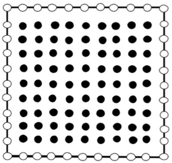
Figure 1.
Boundary element model of the considered problem.
The following material parameters for orthotropic FGM plate are used in numerical analysis: Young’s moduli , Poisson’s ratios shear modulus are
A quadratic variation of the volume fraction is considered with Young’s moduli on the bottom side are: and .
The following material parameters for isotropic FGM plate are used in numerical analysis: Young’s modulus , Poisson’s ratios , the thermal expansion coefficients shear modulus are
We considered numerical results of three-dimensional problem in the computational domain that consists of 40 boundary nodes and 81 internal nodes as shown in Figure 1.
Figure 2, Figure 3, Figure 4, Figure 5, Figure 6 and Figure 7 display the variations of the thermal stress waves , , , , and in the functionally graded (FG) and homogeneous (H) anisotropic fiber-reinforced plates under different values of the fractional order parameter .

Figure 2.
Variation of the thermal stress wave along axis in the functionally graded (FG) and homogeneous (H) anisotropic fiber-reinforced plates under different fractional order parameters.
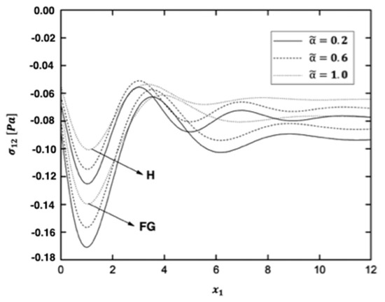
Figure 3.
Variation of the thermal stress wave along axis in the functionally graded (FG) and homogeneous (H) anisotropic fiber-reinforced plates under different fractional order parameters.
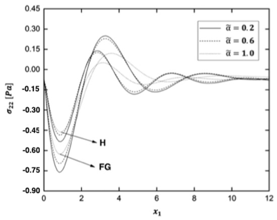
Figure 4.
Variation of the thermal stress wave along axis in the functionally graded (FG) and homogeneous (H) anisotropic fiber-reinforced plates under different fractional order parameters.
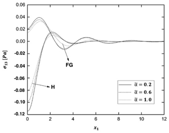
Figure 5.
Variation of the thermal stress wave along axis in the functionally graded (FG) and homogeneous (H) anisotropic fiber-reinforced plates under different fractional order parameters.
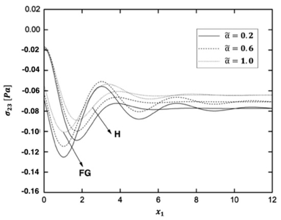
Figure 6.
Variation of the thermal stress wave along axis in the functionally graded (FG) and homogeneous (H) anisotropic fiber-reinforced plates under different fractional order parameters.

Figure 7.
Variation of the thermal stress wave along axis in the functionally graded (FG) and homogeneous (H) anisotropic fiber-reinforced plates under different fractional order parameters.
As shown in Figure 2, the value of the thermal stress wave always increases from a positive value. It grows until it reaches its maximum value in the range. Since then, it has been on a downward trend. Finally, it tends to zero as it moves in the direction of wave propagation. In both FG and H anisotropic fiber-reinforced plates, the thermal stress wave behaves similarly. As shown in Figure 2, the H reduces the maximum value of the thermal stress wave . When the fractional order parameter is varied, the distributions of thermal stress wave are similar.
The thermal stress wave , as shown in Figure 3, has a negative value at and then has a downward trend. It moves in the form of wave propagation after a period of rising. The thermal stress wave behaves similarly in the FG anisotropic fiber-reinforced plate as it does in the H anisotropic fiber-reinforced plate. As shown in Figure 3, the FG fiber-reinforced anisotropic plate increases the minimum value of the thermal stress wave . The distributions of the thermal stress wave are similar when the fractional order parameter is varied.
The thermal stress wave exhibits the same behavior in FG and H anisotropic fiber-reinforced plates, as shown in Figure 4. It demonstrates that the value of the thermal stress wave reaches a negative value early on and has a downward trend. Since then, it has risen from the lowest to the highest point. Finally, it moves in the direction of wave propagation. Figure 4 shows that the maximum value of the thermal stress wave in FG anisotropic fiber-reinforced plates is greater than that in H anisotropic fiber-reinforced plates. The distributions of the thermal stress wave are similar when the fractional order parameter is varied.
In the context of FG anisotropic fiber-reinforced plate, the behavior of the thermal stress wave always goes up from a positive value, as shown in Figure 5. In the FG anisotropic fiber-reinforced plate, the value of the thermal stress wave in the range of is the same as in the FG anisotropic fiber-reinforced plate of Figure 2. From a positive value to its maximum value, it always increases. Then it tends to zero and moves along with the wave. The FG anisotropic fiber-reinforced plate, as shown in Figure 5, increases the amplitude of the thermal stress wave . The distributions of the thermal stress wave are similar when the fractional order parameter is varied.
The thermal stress wave has a negative value at , as shown in Figure 6. The behavior of the thermal stress wave in the FG anisotropic fiber-reinforced plate is identical to that shown in Figure 3. In the absence of gravity, it has a downward trend in the range of . It gradually decreases after a period of rising. As shown in Figure 6, the FG anisotropic fiber-reinforced plate increases the amplitude of the thermal stress wave . When the fractional order parameter is changed, the distributions of the thermal stress wave are similar.
As shown in Figure 7, the behavior of the thermal stress wave in the FG anisotropic fiber-reinforced plate is identical to that of the FG anisotropic fiber-reinforced plate in Figure 4. In the context of H anisotropic fiber-reinforced plate, it always decreases from a negative value at the start. It goes down to its minimum value in the range of , then up from the minimum to the maximum. Finally, as the distance x increases, it tends to zero. As shown in Figure 7, the amplitude of the thermal stress wave is greater in the FG anisotropic fiber-reinforced plate than in the H anisotropic fiber-reinforced plate. The distributions of the thermal stress wave are similar when the fractional order parameter is varied.
Figure 8, Figure 9, Figure 10, Figure 11, Figure 12 and Figure 13 display the variations of the thermal stress waves , σ12, , , and in the functionally graded (FG) and homogeneous (H) plates for anisotropic, orthotropic, and isotropic materials.

Figure 8.
Variation of the thermal stress wave along x1−axis in the functionally graded (FG) and homogeneous (H) fiber-reinforced plates for different materials.
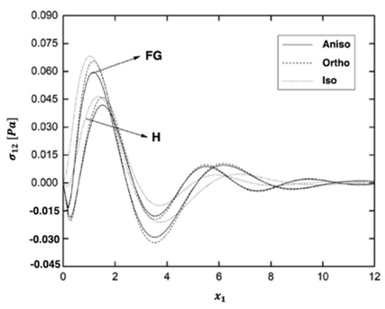
Figure 9.
Variation of the thermal stress wave σ12 along axis in the functionally graded (FG) and homogeneous (H) fiber-reinforced plates for different materials.

Figure 10.
Variation of the thermal stress wave along axis in the functionally graded (FG) and homogeneous (H) fiber-reinforced plates for different materials.
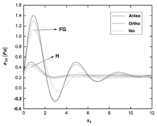
Figure 11.
Variation of the thermal stress wave along axis in the functionally graded (FG) and homogeneous (H) fiber-reinforced plates for different materials.

Figure 12.
Variation of the thermal stress wave σ23 along axis in the functionally graded (FG) and homogeneous (H) fiber-reinforced plates for different materials.

Figure 13.
Variation of the thermal stress wave along axis in the functionally graded (FG) and homogeneous (H) fiber-reinforced plates for different materials.
As shown in Figure 8, the thermal stress wave always rises from a positive starting point. It grows until it reaches its maximum value. It has remained on a downward trend since then. Finally, it moves along with the wave propagation and tends to zero. The thermal stress wave behaves similarly in FG and H fiber-reinforced plates. As illustrated in Figure 8, the homogeneous case reduces the maximum value of the thermal stress wave . The distributions of the thermal stress wave are similar when anisotropic, orthotropic, and isotropic fiber-reinforced plates are considered.
As shown in Figure 9, the thermal stress wave decreases from zero at x = 0 and coincides with the boundary condition. It decreases slightly and then rapidly in the range of . Then it decreases and moves along with the wave. In both the FG and H fiber-reinforced plates, the distributions of the thermal stress wave are similar. The maximum value of the thermal stress wave in the H fiber-reinforced plate is lower than in the FG fiber-reinforced plate, as shown in Figure 9. The distributions of the thermal stress wave are similar when anisotropic, orthotropic, and isotropic fiber-reinforced plates are considered.
As shown in Figure 10, the thermal stress wave begins with a positive value. It begins with an upward trend and reaches its maximum value at . Finally, it decreases and moves as the wave propagates. It behaves similarly in the H and FG fiber-reinforced plates. As illustrated in Figure 10, the H case reduces the maximum value of the thermal stress wave . The distributions of the thermal stress wave are similar when anisotropic, orthotropic, and isotropic fiber-reinforced plates are considered.
As shown in Figure 11, the behavior of the thermal stress wave in the FG case is identical to that shown in Figure 8, it always rises from a positive value. It began with an upward trend and then began to decline. Finally, as the distance x increases, it tends to zero. As shown in Figure 11, the FG fiber-reinforced plate increases the amplitude of the thermal stress wave . The distributions of the thermal stress wave are similar when anisotropic, orthotropic, and isotropic fiber-reinforced plates are considered.
The behavior of the thermal stress wave in the FG fiber-reinforced plate is shown in Figure 12, and it is the same as in the FG fiber-reinforced plate shown in Figure 9. It decreases from zero at to coincide with the boundary condition. It rapidly decreases in the range of and then begins to rise. Finally, it decreases and moves as the wave propagates. As shown in Figure 12, the amplitude of the thermal stress wave is greater in the FG fiber-reinforced plate than in the H fiber-reinforced plate case. The distributions of the thermal stress wave are similar when anisotropic, orthotropic, and isotropic fiber-reinforced plates are considered.
The behavior of the thermal stress wave in the FG fiber-reinforced plate is the same as in the FG fiber-reinforced plate of Figure 10, as shown in Figure 13. In the H fiber-reinforced plate, it falls at first and reaches its lowest point at . Following that, it rises and tends to zero as the distance increases. As shown in Figure 13, the FG fiber-reinforced plate increases the amplitude of the thermal stress wave . The distributions of the thermal stress wave σ33 are similar when anisotropic, orthotropic, and isotropic fiber-reinforced plates are considered.
Figure 14, Figure 15, Figure 16, Figure 17, Figure 18 and Figure 19 display the variations of the thermal stress waves , , , , and in the functionally graded (FG) and homogeneous (H) anisotropic fiber-reinforced plates under different values of the time characteristic of the laser pulse .
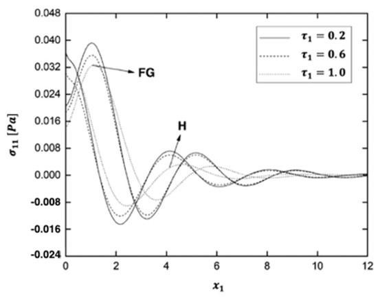
Figure 14.
Variation of the thermal stress wave along axis in the functionally graded (FG) and homogeneous (H) fiber-reinforced plates under different values of time characteristic of the laser pulse.
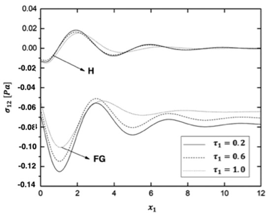
Figure 15.
Variation of the thermal stress wave σ12 along axis in the functionally graded (FG) and homogeneous (H) anisotropic fiber-reinforced plates under different values of time characteristic of the laser pulse.

Figure 16.
Variation of the thermal stress wave along axis in the functionally graded (FG) and homogeneous (H) anisotropic fiber-reinforced plates under different values of time characteristic of the laser pulse.

Figure 17.
Variation of the thermal stress wave σ13 along axis in the functionally graded (FG) and homogeneous (H) anisotropic fiber-reinforced plates under different values of time characteristic of the laser pulse.

Figure 18.
Variation of the thermal stress wave along x1−axis in the functionally graded (FG) and homogeneous (H) anisotropic fiber-reinforced plates under different values of time characteristic of the laser pulse.

Figure 19.
Variation of the thermal stress wave along x1−axis in the functionally graded (FG) and homogeneous (H) anisotropic fiber-reinforced plates under different values of time characteristic of the laser pulse.
As shown in Figure 14, the behavior of the thermal stress wave in the FG anisotropic fiber-reinforced plate is identical to that shown in Figure 5. It reaches its peak in the range , and the value of the thermal stress wave continues to fall. Following that, it tends to zero and moves in the wave propagation. As shown in Figure 14, the time characteristic of the laser pulse influences the behavior of the thermal stress wave . The distributions of the thermal stress wave σ11 are similar when the time characteristic of the laser pulse changes.
As shown in Figure 15, the thermal stress wave in the H anisotropic fiber-reinforced plate has an upward trend in the range of. 0 ≤ x1 ≤ 1.9. When it reaches its maximum value, it gradually decreases and tends to zero. As shown in Figure 15, the time characteristic of the laser pulse causes the value of the thermal stress wave to increase. The distributions of the thermal stress wave are similar when the time characteristic of the laser pulse changes.
As shown in Figure 16, the thermal stress wave decreases slightly and then rapidly increases to its maximum value in the range of . Finally, it approaches zero and moves in the wave propagation. As shown in Figure 16, the time characteristic of the laser pulse causes the maximum value of the FG anisotropic fiber-reinforced plate of thermal stress wave to decrease. The distributions of the thermal stress wave σ22 are similar when the time characteristic of the laser pulse changes.
The thermal stress wave , as shown in Figure 17, decreases from a positive value in the H anisotropic fiber-reinforced plate. In the H anisotropic fiber-reinforced plate, it decreases to its minimum value in the range of . Following that, it grows and moves in the wave propagation. As shown in Figure 17, the FG anisotropic fiber-reinforced plate increases the maximum value of the thermal stress wave σ13. The distributions of the thermal stress wave are similar when the time characteristic of the laser pulse changes.
As shown in Figure 18, the thermal stress wave decreases from zero to coincide with the boundary condition. It rapidly decreases and then increases. Finally, it moves in the direction of wave propagation. Figure 18 shows that the maximum value of the thermal stress wave σ23 in the FG anisotropic fiber-reinforced plate is greater than that in the H fiber-reinforced plate. The distributions of the thermal stress wave are similar when the time characteristic of the laser pulse τ1 changes.
The behavior of the thermal stress wave , as shown in Figure 19, is identical to that shown in Figure 13. In the FG and H anisotropic fiber-reinforced plates, it has a positive value at first. It rises and reaches its highest point at . Then it diminishes and moves in the wave propagation. As shown in Figure 19, the FG anisotropic fiber-reinforced plate increases the maximum value of the thermal stress wave . The distributions of the thermal stress wave σ33 are similar when the time characteristic of the laser pulse takes different values.
Table 2 shows a comparison of required computer resources for the current BEM results, and FEM–NMM results of An et al. [31] for the modeling of ultrasonic wave propagation fractional order boundary value problems of FGA plates.
Table 2.
A comparison of the required computer resources for modeling of ultrasonic wave propagation fractional order boundary value problems of functionally graded anisotropic fiber-reinforced plates.
There were no published results to support the validity of the proposed technique’s findings. Some papers, on the other hand, can be regarded as subsets of the larger study under consideration. The variations of the special case thermal stress waves σ11, σ12, and σ22 along the axis for BEM and combined finite element method/normal mode method (FEM–NMM) in fractional order functionally graded plates are shown in Figure 20, Figure 21 and Figure 22, respectively. These results show that the BEM findings agree very well with the FEM–NMM findings of An et al. [31]. As a result, the proposed technique’s validity was confirmed. We refer the interested readers to the references of fractional derivative of the Riemann Zeta function [32,33,34], fractional derivatives in complex planes [35,36] and fractional boundary element method [37,38].
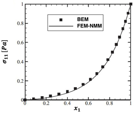
Figure 20.
Variation of the thermal stress wave along x1−axis in the special case of the functionally graded anisotropic fiber-reinforced plates for BEM and FEM-NMM.

Figure 21.
Variation of the thermal stress wave along x1−axis in the special case of the functionally graded anisotropic fiber-reinforced plates for BEM and FEM-NMM.
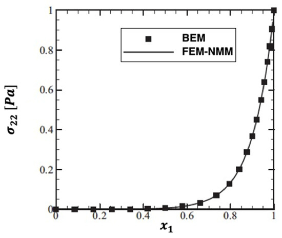
Figure 22.
Variation of the thermal stress wave along x1−axis in the special case of the functionally graded anisotropic fiber-reinforced plates for BEM and FEM-NMM.
6. Conclusions
Some of the conclusions that can be derived from this paper are as follows:
- A numerical BEM scheme based on MLS is applied to FGA fiber-reinforced plates under thermoelastic loads. The Reissner–Mindlin theory, which considers shear deformation, is used to explain the behavior.
- The Laplace-transform is used to remove the time variable from the governing equations.
- The domain under consideration is subdivided into small circular subdomains. The local boundary integral equations are derived using the unit step test function.
- The MLS scheme has been proposed for treating the domain integrals arising from the inertial term and approximates the physical quantities.
- Numerical results demonstrate the accuracy, feasibility, effectiveness, and convergence of the present MLS method.
- The boundary value problems must be solved for a variety of Laplace-transform parameter values chosen for each time instant under consideration.
- The primary benefit of the current technique is its generality and simplicity. The used test function in the proposed technique is less complicated than the fundamental solution for anisotropic fiber-reinforced plates.
- Numerical results demonstrate that the fractional order parameter, functionally graded material, anisotropy, and time characteristic of the laser pulse have significant effects on the thermal stresses of FGA fiber-reinforced plates.
- The numerical results confirm that the proposed technique provides more benefits than other domain discretization methods.
- The results presented in this paper may provide interesting information for researchers who are working on computer science, material science, mathematical physics, geotechnical engineering, and geothermal engineering as well as for those working on the development of the functionally graded anisotropic fiber-reinforced plates.
Funding
This research was funded by Deanship of Scientific Research at Umm Al-Qura University grant number [22UQU4340548DSR04]. The APC was funded by Deanship of Scientific Research at Umm Al-Qura University.
Institutional Review Board Statement
Not applicable.
Informed Consent Statement
Not applicable.
Data Availability Statement
All data generated or analyzed during this study are included in this published article.
Acknowledgments
The author would like to thank the Deanship of Scientific Research at Umm Al-Qura University for supporting this work by Grant Code: (22UQU4340548DSR04).
Conflicts of Interest
The author declares no conflict of interest.
Appendix A
Table A1.
Nomenclature.
Table A1.
Nomenclature.
| Strain | Young’s moduli | ||
| & | Elastic parameters | Shear moduli | |
| ρ (x) | Mass density | Non-Gaussian temporal profile | |
| Temperature field | Total energy intensity | ||
| Stress | Thermal conductivity tensor | ||
| Laser pulse time characteristic | n | Functionally graded parameter | |
| MLS shape functions | Generic property | ||
| LRBF shape functions | Pb | Bottom face property | |
| Fractional order parameter | Top face property | ||
| Linear thermal expansion coefficients | Q(x,t) | Heat source intensity | |
| Specific heat | R | Irradiated surface absorptivity | |
| Material stiffness coefficients | Poisson’s ratios |
References
- Podlubny, I. Fractional Differential Equations; Academic Press: San Diego, CA, USA, 1999. [Google Scholar]
- Kilbas, A.A.; Srivastava, H.M.; Trujillo, J.J. Theory and Applications of Fractional Differential Equations; Elsevier Science: Amsterdam, The Netherlands, 2006; Volume 204. [Google Scholar]
- Sabatier, J.; Agrawal, O.P.; Machado, J.A.T. (Eds.) Advances in Fractional Calculus: Theoretical Developments and Applications in Physics and Engineering; Springer: Dordrecht, The Netherlands, 2007. [Google Scholar]
- Ortigueira, M.D.; Machado, J.A.T.; Da Costa, J.S. Which differintegration? IEE Proc. Vis. Image Signal Processing 2005, 152, 846–850. [Google Scholar] [CrossRef] [Green Version]
- Lancaster, P.; Salkauskas, K. Surfaces generated by moving least squares methods. Math. Comput. 1981, 37, 141–158. [Google Scholar] [CrossRef]
- Levin, D. The approximation power of moving least-squares. Math. Comput. 1998, 67, 1517–1531. [Google Scholar] [CrossRef] [Green Version]
- Palermo, L., Jr. A Study About Fundamental Solution in Plates; WIT Press: Ashurst Lodge, UK, 2000. [Google Scholar]
- Mindlin, R.D. Influence of rotatory inertia and shear on flexural motions of isotropic elastic plates. J. Applled Mechunlcs 1951, 18, 31–38. [Google Scholar] [CrossRef]
- Reissner, E. The Effect of Transverse Shear Deformation on the Bending of Elastic Plates. J. Appl. Mech. 1945, 12, A69–A77. [Google Scholar] [CrossRef]
- Wang, J.; Huang, M. Boundary element method for orthotropic thick plates. Acta Mech. Sin. 1991, 7, 258–266. [Google Scholar]
- Belytschko, T.; Krogauz, Y.; Organ, D.; Fleming, M.; Krysl, P. Meshless methods; an overview and recent developments. Comput. Methods Appl. Mech. Eng. 1996, 139, 3–47. [Google Scholar] [CrossRef] [Green Version]
- Donning, B.M.; Liu, W.K. Meshless methods for shear-deformable beams and plates. Comput. Methods Appl. Mech. Eng. 1998, 152, 47–71. [Google Scholar] [CrossRef]
- Krysl, P.; Belytschko, T. Analysis of thin shells by the element-free Galerkin method. Int. J. Solids Struct. 1996, 33, 3057–3080. [Google Scholar] [CrossRef]
- Fahmy, M.A. A new boundary element formulation for modeling and simulation of three-temperature distributions in carbon nanotube fiber reinforced composites with inclusions. Math. Methods Appl. Sci. 2021, in press. [Google Scholar] [CrossRef]
- Fahmy, M.A.; Alsulami, M.O. Boundary element and sensitivity analysis of anisotropic thermoelastic metal and alloy discs with holes. Materials 2022, 15, 1828. [Google Scholar] [CrossRef] [PubMed]
- Ezzat, M.A.; Youssef, H.M. Generalized magneto-thermoelasticity in a perfectly conducting medium. Int. J. Solids Struct. 2005, 42, 6319–6334. [Google Scholar] [CrossRef] [Green Version]
- Abouelregal, A.E.; Mohammed, W.W. Effects of nonlocal thermoelasticity on nanoscale beams based on couple stress theory. Math. Methods Appl. Sci. 2020, in press. [Google Scholar] [CrossRef]
- Fahmy, M.A.; Shaw, S.; Mondal, S.; Abouelregal, A.E.; Lotfy, K.; Kudinov, I.A.; Soliman, A.H. Boundary element modeling for simulation and optimization of three-temperature anisotropic micropolar magneto-thermoviscoelastic problems in porous smart structures using NURBS and genetic algorithm. Int. J. Thermophys. 2021, 42, 29. [Google Scholar] [CrossRef]
- Fahmy, M.A. A new boundary element algorithm for modeling and simulation of nonlinear thermal stresses in micropolar FGA composites with temperature-dependent properties. Adv. Modeling Simul. Eng. Sci. 2021, 8, 6. [Google Scholar] [CrossRef]
- Fahmy, M.A. Boundary element modeling of fractional nonlinear generalized photothermal stress wave propagation problems in FG anisotropic smart semiconductors. Eng. Anal. Bound. Elem. 2022, 134, 665–679. [Google Scholar] [CrossRef]
- Fahmy, M.A. Boundary element modeling of 3T nonlinear transient magneto-thermoviscoelastic wave propagation problems in anisotropic circular cylindrical shells. Compos. Struct. 2021, 277, 114655. [Google Scholar] [CrossRef]
- Atluri, S.N. The Meshless Method (MLPG) For Domain & BIE Discretizations; Tech Science Press: Norcross, GA, USA, 2004. [Google Scholar]
- Sladek, J.; Sladek, V.; Mang, H.A. Meshless formulations for simply supported and clamped plate problems. Int. J. Numer. Methods Eng. 2002, 55, 359–375. [Google Scholar] [CrossRef]
- Sladek, J.; Sladek, V.; Mang, H.A. Meshless LBIE formulations for simply supported and clamped plates under dynamic load. Comput. Struct. 2003, 81, 1643–1651. [Google Scholar] [CrossRef]
- Soric, J.; Li, Q.; Jarak, T.; Atluri, S.N. Meshless Local Petrov-Galerkin (MLPG) Formulation for Analysis of Thick Plates. CMES Comput. Modeling Eng. Sci. 2004, 6, 349–358. [Google Scholar]
- Sladek, J.; Sladek, V.; Wen, P.H.; Zhang, C. Modelling of plates and shallow shells by meshless local integral equation method. In Boundary Element Methods in Engineering and Sciences, 1st ed.; Aliabadi, M.H., Wen, P.H., Eds.; Imperial College Press: London, UK, 2010; Volume 4, pp. 197–238. [Google Scholar]
- Horváth, I.; Talyigás, Z.; Telek, M. An Optimal Inverse Laplace Transform Method Without Positive and Negative Overshoot–An Integral Based Interpretation. Electron. Notes Theor. Comput. Sci. 2018, 337, 87–104. [Google Scholar] [CrossRef]
- Reissner, E. Stresses and Small Displacements of Shallow Spherical Shells. I. J. Math. Phys. 1946, 25, 80–85. [Google Scholar] [CrossRef]
- Wang, B. A local meshless method based on moving least squares and local radial basis functions. Eng. Anal. Bound. Elem. 2015, 50, 395–401. [Google Scholar] [CrossRef]
- Chowdhury, H.A.; Joldes, G.R.; Wittek, A.; Doyle, B.; Pasternak, E.; Miller, K. Implementation of a Modified Moving Least Squares Approximation for Predicting Soft Tissue Deformation using a Meshless Method. In Computational Biomechanics for Medicine; Doyle, B., Miller, K., Wittek, A., Nielsen, P., Eds.; Springer: Cham, Switzerland, 2015; pp. 59–71. [Google Scholar] [CrossRef]
- An, B.; Zhang, C.; Shang, D.; Xiao, Y.; Khan, I.U. A Combined Finite Element Method with Normal Mode for the Elastic Structural Acoustic Radiation in Shallow Water. J. Theor. Comput. Acoust. 2020, 28, 2050004. [Google Scholar] [CrossRef]
- Guariglia, E. Fractional calculus, zeta functions and Shannon entropy. Open Math. 2021, 19, 87–100. [Google Scholar] [CrossRef]
- Guariglia, E. Riemann zeta fractional derivative-functional equation and link with primes. Adv. Differ. Equ. 2019, 1, 261. [Google Scholar] [CrossRef]
- Torres-Hernandez, A.; Brambila-Paz, F. An approximation to zeros of the Riemann zeta function using fractional calculus. Math. Stat. 2021, 9, 309–318. [Google Scholar] [CrossRef]
- Zavada, P. Operator of fractional derivative in the complex plane. Commun. Math. Phys. 1998, 192, 261–285. [Google Scholar] [CrossRef] [Green Version]
- Li, C.; Dao, X.; Guo, P. Fractional derivatives in complex planes. Nonlinear Anal. Theory Methods Appl. 2009, 71, 1857–1869. [Google Scholar] [CrossRef]
- Fahmy, M.A. A new boundary element algorithm for a general solution of nonlinear space-time fractional dual-phase-lag bio-heat transfer problems during electromagnetic radiation. Case Stud. Therm. Eng. 2021, 25, 100918. [Google Scholar] [CrossRef]
- Fahmy, M.A. A New BEM for Fractional Nonlinear Generalized Porothermoelastic Wave Propagation Problems. CMC Comput. Mater. Contin. 2021, 68, 59–76. [Google Scholar]
Publisher’s Note: MDPI stays neutral with regard to jurisdictional claims in published maps and institutional affiliations. |
© 2022 by the author. Licensee MDPI, Basel, Switzerland. This article is an open access article distributed under the terms and conditions of the Creative Commons Attribution (CC BY) license (https://creativecommons.org/licenses/by/4.0/).