Article

Fractional Variation Network for THz Spectrum Denoising without Clean Data

1
School of Optics and Photonics, Beijing Institute of Technology, Beijing 100081, China
2
Beijing Key Laboratory for Precision Optoelectronic Measurement Instrument and Technology, Beijing 100081, China
3
Yangtze Delta Region Academy of Beijing Institute of Technology, Jiaxing 314019, China
*
Author to whom correspondence should be addressed.
Fractal Fract. 2022, 6(5), 246; https://doi.org/10.3390/fractalfract6050246
Submission received: 21 February 2022 / Revised: 20 April 2022 / Accepted: 28 April 2022 / Published: 29 April 2022
(This article belongs to the Special Issue Recent Advances in Computational Physics with Fractional Application)

Abstract

:
Deep learning can remove the noise of the terahertz (THz) spectrum via its powerful feature extraction ability. However, this technology suffers from several limitations, including clean training data being difficult to obtain, the amount of training data being small, and the restored effect being unsatisfactory. In this paper, a novel THz spectrum denoising method is proposed. Low-quality underwater images and transfer learning are used to alleviate the limitation of the training data amount. Then, the principle of Noise2Noise is applied to further reduce the limitations of clean training data. Moreover, a THz denoising network based on Transformer is proposed, and fractional variation is introduced in the loss function to improve the denoising effect. Experimental results demonstrate that the proposed method estimates the high-quality THz spectrum in simulation and measured data experiments, and it also has a satisfactory result in THz imaging.

1. Introduction

Many industrial fields [1], such as materials [2,3], chemistry [4], biological, and medical fields [5,6], are commonly monitored via adopting the terahertz (THz) spectroscopy method. The prominent penetrative capability of THz radiation makes the THz spectrum a powerful tool in the above fields. However, the accuracy of qualitative and quantitative analysis via THz spectroscopy is restricted because of the instrumentation or environmental factors [7,8]. Therefore, high-quality THz spectra play a crucial role in the above fields.
Generally, increasing the integration time is an acceptable method to remove noise. However, this method is inefficient because the integration time is used for all sampling points rather than the high-noise region. The applications, such as raster-scan imaging or monitoring a fast dynamic process [9], are restricted severely by increasing the integration time because these need a swift acquisition process. To lower the integration time, many methods based on digital signal processing technology have been proposed. Pupeza et al. [10] proposed a spatially variant moving average filter (SVMAF) to improve the quality of reconstructed THz spectra. Shen et al. proposed a signal reconstruction method using compressed sensing and a Savitzky–Golaysgz filter [11]. Khani et al. [12] retrieved the spectral absorption fingerprints of α-lactose monohydrate and 4-aminobenzoic acid in rough surfaces via phase function corrections and the hard threshold. These works prove the practicability of digital signal processing. Zeng et al. [13] utilized the Bézier curve and B-spline to smooth the noise, and this method is preferable for THz signal stability and robustness. Wang et al. [14] proposed a THz radar signal denoising algorithm by using adaptive empirical mode decomposition and stochastic resonance system. Liu et al. [15] believe that IR spectrum reconstruction can be considered a maximum a posteriori (MAP)-based problem. They solved this problem by minimizing a cost function, which included a likelihood term and two prior terms. Chen et al. [16] mitigated the noise effect via reconstructing the transfer function based on the genetic algorithm. The reconstructed THz spectra are more objective than the above methods because this method does not require thresholds. In general, the above works, which have obtained impressive reconstructed spectra, are based on noise prior. The noise prior assumes that noise increases the gradient of the THz spectrum, and noise belongs to the high-frequency signal in the frequency or wavelet domain. Unfortunately, noise is mixed with the actual high-frequency signal, and it is difficult to separate the noise from the captured THz spectrum in the frequency domain or wavelet domain. This problem may lead to the reconstructed THz spectrum being over-smooth or residual noise. Deep learning is a feasible method to alleviate these problems.
Deep learning technology [17] has attracted growing attention because of its formidable nonlinear fitting ability and feature extraction [18] ability. These advantages make deep learning a better method to separate the noise from the real signal than noise prior. Nowadays, it has been applied to optical imaging systems [19], blind deblurring [20], and image denoising [21] outstandingly. Currently, deep-learning-based methods, convolutional neural network (CNN)-based methods especially, have been preliminarily applied in spectral pre-processing. Pan et al. [22] removed the noise of Raman spectra. Joel et al. [23] implemented single-step preprocessing using a CNN. Jiao et al. [24] also designed a CNN-based method to remove noise and baseline. These methods can estimate a high-quality spectrum and have been applied in chemometrics. However, there are two crucial problems to limit the development of deep learning in THz spectra. One of the problems is the dataset [25]. Deep learning usually requires an extremely large amount of data for training, and the more data there is, the better the effect of the deep learning model. However, it is difficult to establish an excellent dataset, which is expensive and time-consuming. Another problem is that it is impossible to capture the ideal THz spectra due to temperature, humidity [26], cosmic radiation [27], and other factors. However, when training the deep learning network, a clean terahertz spectrum is necessary because the network model needs to establish the mapping relationship between noisy and clean THz spectra. These problems restrict the application of deep learning in THz spectral denoising.
To alleviate the aforementioned problems and improve the quality of the restored THz spectrum, a THz spectrum denoising method without clean data is proposed. In this study, the most general condition is applied, which only provides a contaminated THz spectrum to train and test the proposed method. The main solutions of the above problem and contributions of the proposed method can be summarized as follows.
(1)
The most significant difference between the proposed method and the state-of-the-art deep-learning-based methods is that the proposed method can estimate the clean THz spectrum without clean data.
(2)
Fractional variation is introduced to the L2 loss function, which can improve the restored quality and avoid the failure of the L2 loss function.
(3)
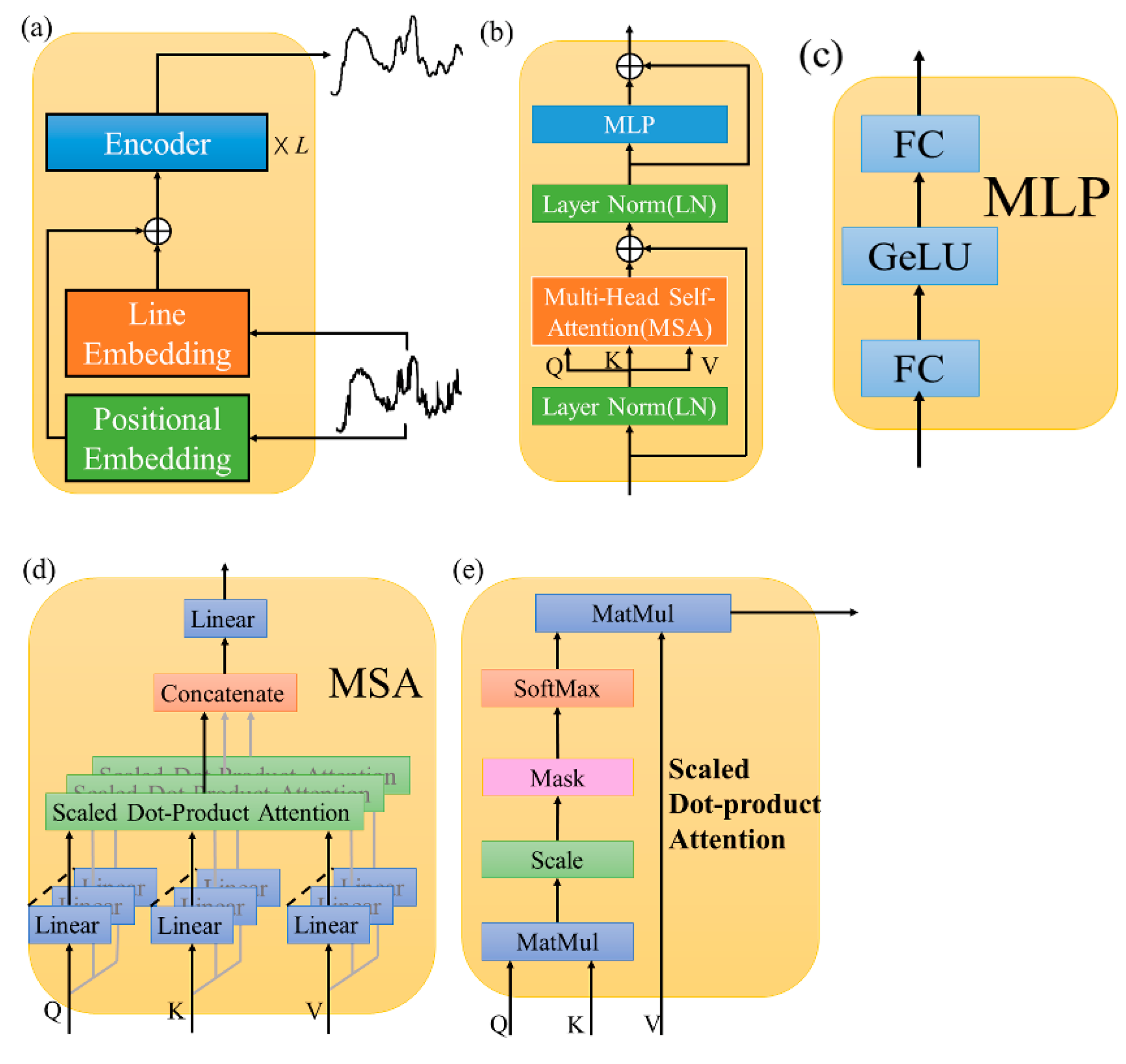
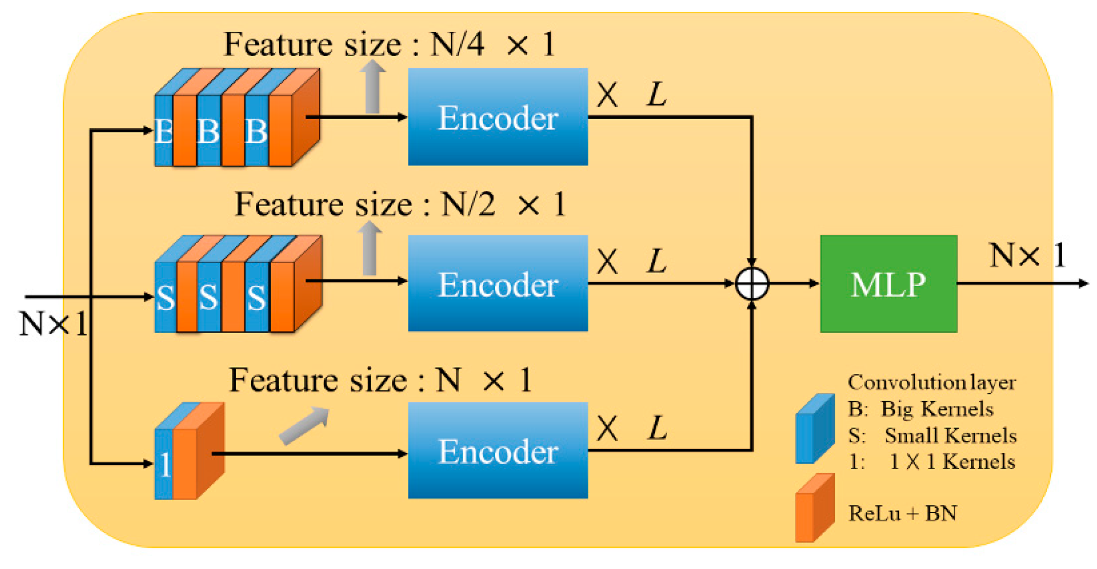
To estimate the high-quality THz spectrum, the Transformer network is applied, and it is modified to a multi-stream feature fusion network to remove the noise of the THz spectrum. Notably, the Transformer network is a potent natural language processing architecture.
(4)
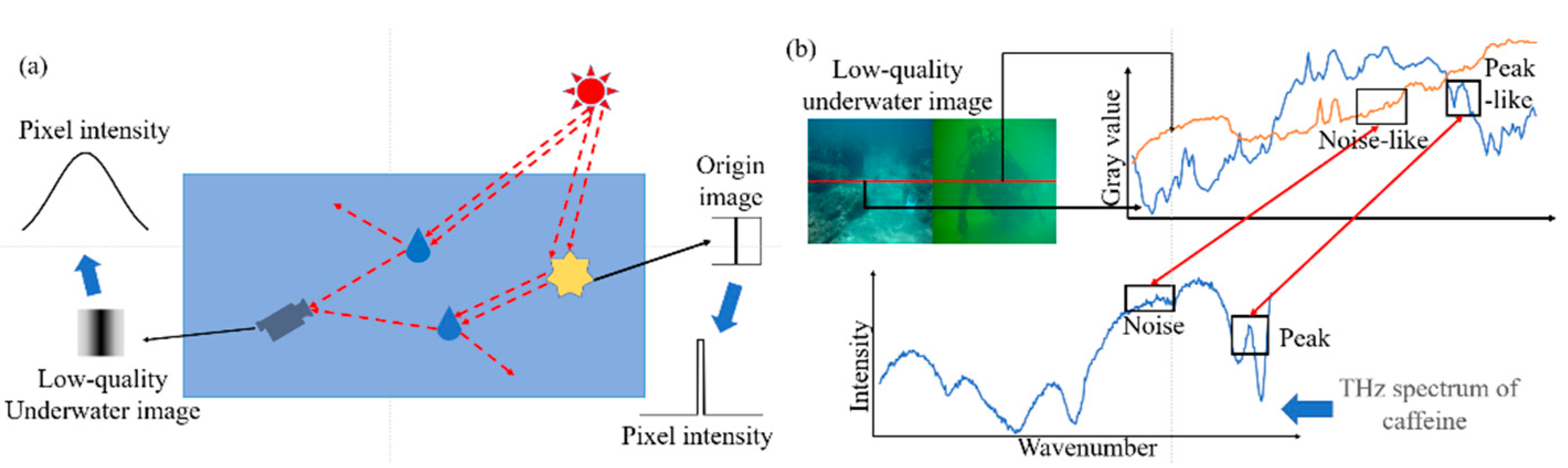
To augment the training data, a low-quality underwater image is applied. Transfer learning is used to prevent signal offset of the low-quality image.
(5)
The synthesized data, measured THz spectrum, and THz imaging are utilized to verify the performance of the proposed methods.

2. Methods

Figure 1 illustrates the distinction between the conventional methods and our method. Unlike the traditional deep-learning-based spectrum denoising framework, the proposed method does not require numerous different samples to obtain the THz spectrum, and does not require too long an integration time to capture the high-SNR THz signal, which can save cost and improve efficiency.

2.1. THz Spectra Line Type

Generally, the THz spectrum consists of three different signals. Background signals comprise the flat region that has no feature peak. The intensity of background signals is approximate to their neighborhood points. Noise signals are random and impact the THz spectrum application, such as chemometrics [28]. Feature peak signals comprise the most valuable region in qualitative and quantitative analysis, and their intensity varies dramatically. In practice, the feature peak signals can be described by Gauss or Lorentz functions [29]. To model the spectral structure efficiently, the feature peak can be regarded as a Voigt function [30], and this function can be expressed as
V ( ν ) = k ε exp [ ( ν ν 0 ) 2 α L 2 ] + ( 1 k ) β L π [ ( ν ν 0 ) 2 + β L 2 ] ,
where k is the synthetic factor, k [ 0 , 1 ] , v 0 is the center frequency of the THz spectra, ε is the peak value, and α L and β L are the half peak width of Gauss and Lorentz functions, respectively. From (1), the first term is a Gauss function, and the second term is a Lorentz function. This shows that the spectral peak is symmetrical.

2.2. Transfer Learning

Transfer learning [31], which concentrates on transferring the knowledge from source domains to target domains, is a state-of-the-art deep learning technology. It is universal that pianists can learn the violin more easily than soccer players, and soccer players can study basketball faster than pianists. This is because learning the piano and violin (soccer and basketball) involves common knowledge or experience. Analogously, it is hypothesized that the image and THz spectrum have the same type of structure and noise. In practice, the source domain is the low-quality underwater image and the target domain is the THz spectrum. The similarity of structure and noise from the underwater images and the THz spectra is discussed below, and the quantitative analysis is shown in Section 3.2.
Structure: Theoretically, THz waves and visible light have different physical properties. However, in 1-D data (the coordinate system of wavelength-spectral intensity and pixel coordinates-pixel intensity), the THz spectrum and low-quality underwater image have similar mathematical properties, such as gradient, concavity-convexity, and extremal properties. Specifically, the strong peak, baseline, and weak peak in a THz spectrum, which are generated by the physical property THz waves, and sharp edges, background, and blurred edges in the image have similar mathematical characteristics. To enhance similarity, low-quality underwater images are applied as source fields for transfer learning. Due to the refraction of light by the impurities in the water [32], the sharp edges in the original image can become gentle inclines, and the weak edges can become more blurred, becoming peak-like and noise-like regions, respectively. The illustration of the impact of water is shown in Figure 2a. In practice, we convert the RGB underwater images to grayscale images, and then select a row to observe its intensity. The schematic can be seen in Figure 2b.
From Figure 2b, the low-quality underwater images are at the top left. The relation between gray value and column coordinate is at the top right. The THz spectrum can be seen at the bottom of Figure 2b. According to Figure 2b, the noisy-like and peak-like regions exist in the relation between gray value and column coordinate, and similarity between noise and noise-like (peak and peak-like) regions is the basis of transfer learning.
Noise: Theoretically, the underwater images and THz spectra are disturbed by noise, which comes from the inside of the instrument (optical imaging system or spectrometer) or factors such as temperature and dust. The noise values generated by these factors are random and independent of each other. Hence, the synthesis noise is subject to the Gaussian distribution due to the central limit theorem. Therefore, the underwater images and THz spectra may have the same type of noise.

2.3. Loss Function with Fractional Order Differential

In this section, the improved loss function is introduced. Firstly, the theory of the proposed denoising method without clean data is explained. Then, the fractional order variation is applied to improve the loss function.
The proposed method is inspired by Noise2Noise (N2N) [33], and N2N is an image denoising algorithm that achieves high-quality images without using any clean image to train the network. In the training phase, the input and output of the network are different noisy data, which are obtained via adding the noise with different SNRs to the same data. Generally, L2 loss can be expressed as (2), and it is a conventional loss function in deep learning. In the proposed method, the loss function can be rewritten as (3).
θ = arg min θ E x [ f ( y 1 ; θ ) x 2 ] ,
where x is the ideal THz spectrum, y1 and y2 are the noisy THz spectra, f(y1;θ) is the deep learning model, and θ denotes the parameters of the deep learning model. From (2), the conditional expectation of the expansions of the L2 loss can be described as
E y | x [ f θ ( y 1 ; θ ) x 2 ] = E y | x [ f ( y 1 ; θ ) 2 ] 2 x T E y | x [ f ( y 1 ; θ ) ] + x 2 ,
E y | x [ f θ ( y 1 ; θ ) y 2 2 ] = E y | x [ f ( y 1 ; θ ) 2 ]   2 E y | x ( y 2 ) T E y | x [ f ( y 1 ; θ ) ] + E y | x ( y 2 2 ) ,
E y | x ( y 2 ) = x .
From (3) and (4), it is necessary to satisfy the condition (5). Therefore, the proposed method must meet two assumptions. One of the assumptions is that the arithmetic mean of clean data is equal to the noisy data. This assumption signifies the noise is zero-mean, which is acceptable because of the central limit theorem. Another assumption is that the two noisy data need to be decorrelated or completely uncorrelated. In practice, the multiple different zero-mean artificial random noise values are randomly added to the same THz spectrum. Then, two THz spectra with the lowest correlation are selected as the training set. In the training phase, the proposed method is divided into three stages, noise data generation, pre-training via the underwater image, and fine-training via the noisy THz spectrum.
The input and output of the proposed method are noisy THz spectra in training, and L2 loss (2) only involves similarity between data. Therefore, the proposed method may be useless if the noisy spectra are very similar. To avoid this problem and improve the denoising effect, the fractional variation is an advisable tool.
In recent years, the fractional-variation-based method has been successfully applied in signal processing [34,35] due to its advantage over the existing methods. In previous work, both integer and fractional-order operators can extract the high-frequency features effectively. Nevertheless, only fractional differential operators can improve the details of the low-frequency region [36]. This advantage of fractional differential operators can preserve the weak peaks and overlapping peaks from noise.
However, unlike integer-order differential operators, fractional-order differential operators do not have a unified definition. There are three representative definitions: Grünwald–Letnikov, Riemann–Liouville, and Caputo [37]. To reduce the computational complexity of proposed method, the Grünwald–Letnikov differential operator is used in this paper, because this operator has the strength that it can convert to convolution, which is suitable for processing a 1-D discrete signal such as a spectrum, in numerical implementation.
Therefore, the improved loss function via fractional variation is described as
θ = arg min θ E x [ f ( y 1 ; θ ) y 2 2 + λ D α f ( y 1 ; θ ) 2 2 ] ,
D α V ( v ) V ( v ) + ( α ) V ( v 1 ) + ( α ) ( 1 α ) 2 f ( v 2 ) + + Γ ( 1 α ) n ! Γ ( 1 α + n ) f ( t n ) ,
where λ is the regularization parameter, D α is the Grünwald–Letnikov fractional differential operator, α is the order number, V ( · ) is the spectrum function, v is the wavelength, and Γ ( · ) is the gamma function, which is a meromorphic function defined in the range of complex numbers.

2.4. Transformer

To estimate the clean THz spectrum, the Transformer network is used to remove noise [38]. The Transformer network has been a great success in natural language processing. Designed for sequence modeling and transduction tasks, the Transformer is notable for its use of attention to model long-range dependencies in the data. Recently, the Vision Transformer [39] has also proved that a pure Transformer architecture can achieve state-of-the-art performance in the computer vision field when the training data are large enough. However, it is incredible that the Transformer net has hardly been applied to spectral analysis and applications. According to Section 2.1, the different regions may have the same features in THz spectra. For example, the different peaks may have the same line type, and this means that non-local or long-range data can provide more useful information than local data for tasks such as denoising. Theoretically, the non-local similarity [40] is a powerful tool to remove noise. Therefore, the Transformer, which specializes in global modeling, is an ideal approach to obtain clean THz spectra, and Figure 3 shows the architecture of the Transformer.
Figure 3a shows the architecture of the Transformer, and Figure 3b shows the architecture of the Transformer encoder layer (MSA), where Figure 3c,d show the structure of the MLP layer and multi-head self-attention layer, and Figure 3e shows the structure of the scaled dot-product attention layer. From Figure 3a, the noisy THz spectrum is calculated via the line embedding layer and positional embedding layer. Then, the result of the addition of the line embedding layer and positional embedding layer is the input to the encoding layer. Finally, the clean THz spectra can be obtained via multiple encoding layers.
In Transformer net, the encoding layer is the paramount module, and its architecture is shown in Figure 3b. Firstly, the input data pass the line norm layer to obtain three sequences: query (Q), key (K), and value (V). Then, Q, K, and V pass the multi-head self-attention layer (MSA), and the result and input data are added as the input of the second norm layer in the encoding layer. Finally, the output of the encoding layer can be calculated via multilayer perceptron (MLP, Figure 3c), and the input of MLP is the output of the second norm layer. The mathematical model of the encoding layer and MLP are described as
z l 0.5 = MAS ( LN ( z l 1 ) ) + z l 1 ,   l = 1 , 2 L ,
z l = MLP ( LN ( z l 0.5 ) ) + z l 0.5 ,   l = 1 , 2 L ,
MLP ( z ) = FC ( GeLu ( FC ( z ) ) ) ,
where z represents the input data of the Transformer encoding layer, and L is the number of encoding layers. FC is the fully connectional layer, and GeLu is the activation function.
MSA is the vital component of the Transformer, and its concrete structure is shown in Figure 3d. Firstly, Q, K, and V pass the linear layers. Then, the results are calculated via the scaled dot-product attention layer. Finally, the output of MAS is obtained via a concatenation layer and a linear layer. The concatenation layer can concatenate the outputs of the scaled dot-product attention layer.
In practice, the self-attention map, which is the output of the MSA module, can be regarded as a weight map. The scaled dot-product attention layer is the core in the MSA module, which estimates the attention map via computing the Q, K, and V scaling dot-product. Figure 3e shows the details of the scaled dot-product attention layer. Firstly, the dot product of Q and K is calculated to determine the relevance between an element with other elements on the input data. Then, the result is scaled and fed into a softmax block to enhance useful features and discard futile features. Finally, the output of softmax is multiplied via V to procure the self-attention map. Therefore, the mathematical model of the scaled dot-product attention layer can be described as
[ Q , K , V ] = z U Q , K , V = FC ( z ) ,
SA ( z ) = softmax ( Q K T D ) V ,
where D is the dimension of K and U is a learnable parameter vector; U can be replaced via the fully connected layer or 1 × 1 convolutional layer.
The structure of the improved Transformer is shown in Figure 4. Apparently, the language is the information-intensive data, but the spectrum has sparsity, and useful information is contained in the spectral peaks. Therefore, it is vital to improve the Transformer network.
Furthermore, THz spectral sparsity is the main reason for the network design. The information from the uppermost stream is the densest, which can provide the most global and non-local information. The lowest stream has the richest local information, which is complementary to the uppermost flow. The middle stream is the supplement of other streams. Similarly, the uppermost stream can output the feature of the highest resolution, and the lowest stream can obtain the most abstract feature. Therefore, the proposed method can fuse different features to estimate the high-quality THz spectrum.

3. Experiments

In this section, we train and test the proposed method on synthetic and measured THz spectra. The training dataset and details are introduced in Section 3.1. Then, the similarity between low-quality underwater images and THz spectra are quantitatively analyzed in Section 3.2. The performance of the proposed method is verified via simulation experiment and measured THz spectrum, which are proved in Section 3.3 and 3.4, respectively. In Section 3.5, the performance of data augmentation using low-quality underwater images is compared. The effect of a fractional-order loss function is introduced in Section 3.6. In Section 3.7, the proposed method is applied to the reconstruction of THz imaging.

3.1. Training Dataset and Detail

In experiments, the training data contain two parts, the low-quality underwater images and the noisy THz spectrum. The underwater images are from the UIEB dataset [41], which has 890 raw underwater images with corresponding high-quality reference images and 60 poor-quality underwater images. Part of the THz spectrum includes the collected spectra at different temperatures and humidities, which have noise but no reference data. The other part of the spectrum is from the Internet, for example, the NIST Standard Reference Database [42] and figshare [43], and these data comprise clean signals.
The network, for which the size of input is 256 × 1, is implemented via Tensorflow. The network is trained on a server equipped with a single NVIDIA V100 GPU. The rest of the training setup is the same as for N2N, and the training model is long train, which is a Boolean optional parameter of N2N. In addition, the encoder quantity of the large convolution kernel channel is 13, the encoder quantity of the small convolution kernel channel is 9, and the encoder quantity of the 1 × 1 convolution kernel channel is 5.

3.2. Pre-Train Image

Firstly, the different types of images are used to pre-train the network. In this part, the underwater image, high-quality natural image (including the high-quality underwater image), and nighttime image are used as the experimental data. In this section, the test images are resized to 256 × 256.
To evaluate the similarity between images and the THz spectrum, the structural similarity (SSIM), correlation coefficient (R2), and the p of the t-test are applied as merits. The tested data include clean THz spectra, which are from NIST, and synthetic spectra. The THz spectra are resized to 256 × 1. To improve generality, the number of tested images is much greater than the training images. In this part, we use the low-quality underwater image, high-quality natural image, and nighttime image. Secondly, to test the training effect, the above images are used to train the proposed network. The R2, root-mean-square error (RMSE), and signal-to-noise ratio (SNR) are used as evaluation indexes. Table 1 shows the results for SSIM and R2, and Table 2 shows the restored effect via different types of training images.
Table 1 shows the similarity between the THz spectrum and images, which is the basis of transfer learning. From the SSIM, the low-quality underwater images have the max value, which means that the edge, background of images, and the peak, flat region of THz spectrum are similar. Especially, the low-quality underwater images have the highest SSIM score. The highest SSIM shows that the image edges become blunt, caused by scattering of impurities in water, which makes the edge of the underwater image have a similar structure to the THz spectrum peak; the image background also becomes dim, which is caused by the attenuation of light in water, giving the background of the underwater image a similar intensity to the THz spectrum flat region. From R2, the correlation between image and spectrum is poor. The low correlation means these two types of data rarely rise or fall in tandem. This is a normal phenomenon as the number of test images increases. The p of the t-test shows that the statistical significance of the image and THz spectrum is strong, which indicates that the difference between image data and THz data is small. Therefore, the low-quality underwater images are a suitable choice to be used for transfer learning.
Table 2 displays the denoising effect. The result demonstrates that using images to pre-train the proposed method is an effective tool to remove noise. Excellent results can be obtained by using low-quality underwater images for pre-training. Hence, the low-quality underwater image may be a practical tool to expand the THz spectrum for pre-training.

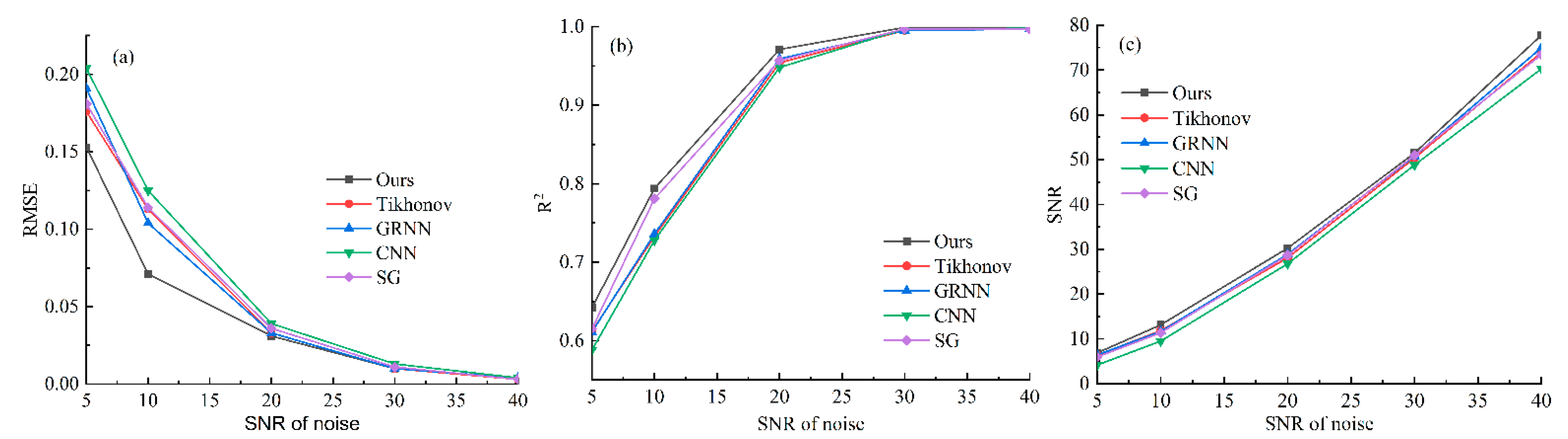
3.3. Simulation Experiment

In this section, Tikhonov regularization [44], a convolutional neural network (CNN) [20], generalized regression neural network (GRNN) [45], and Savitzky–Golay filter (SG) [46] are compared with the proposed methods. These methods include deep learning (GRNN, CNN) and blind deconvolution (Tikhonov, and SG). GRNN and CNN involve supervised learning, which needs clean data to train the network. Tikhonov and SG are non-deep-learning-based methods, which can remove noise without clean data. Therefore, these methods can evaluate the proposed method from two aspects: deep learning and no clean data. In this experiment, the RMSE, R2, and SNR are evaluation indexes. Regarding the synthetic spectrum, the number of peaks is selected randomly between 5 and 17, and the line type of the peak is Gaussian, in which height and half peak width are selected randomly. For generality, 1000 synthetic spectra are applied, and they are added to the different SNR of noise.
Figure 5 shows the experimental results of RMSE, R2 and SNR. The proposed method shows excellent performance. Firstly, when the noise is low, all methods estimate the similar and high-quality reconstructed spectrum. Secondly, when the appropriate SNR noise is added, the proposed method is still the best, and the SG filter and Tikhonov effect are similar. Finally, when the noise is high, the proposed method still has some denoising ability.
To intuitively evaluate the performance of the proposed method, Figure 6a shows the noisy synthetic spectrum and Figure 6b–f show the denoising result via the proposed method, Tikhonov, GRNN, CNN, and SG filter. Table 3 shows the error of the synthetic peak.
From Figure 6, each method has a similar restored effect of independent spectral peaks. However, the CNN is the worst because it has strength loss in the second and third peaks. From Figure 6, the second and third peaks are overlapping peaks, and the intensity of the second peak is the lowest. For overlapping or weak peaks, the proposed method can estimate the highest-quality spectral peak. The loss of spectral intensity and the shift of spectral peak position exists in other methods, which shows that the proposed method can achieve the best results.
The quantitative analysis of the restored spectral peak is shown in Table 3. For overlapping or weak peaks, the proposed method has the best performance. Regarding strong peaks, all denoising results are similar. All restored effects have a little bit of deviation or residual noise, but the proposed method has the best performance from Figure 6. According to the above results, the proposed method can estimate the most precise spectrum peak.

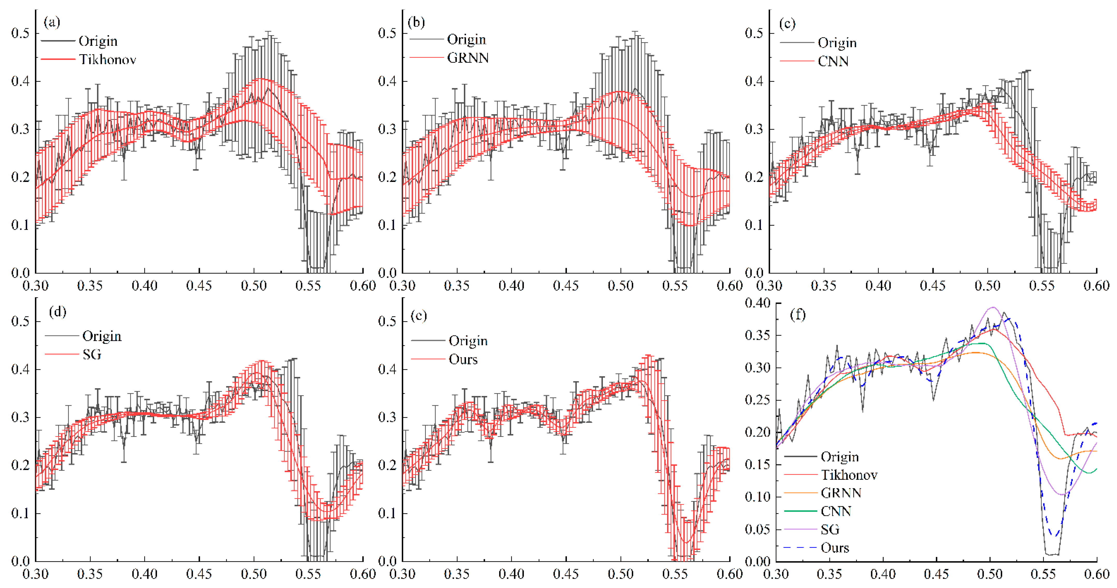
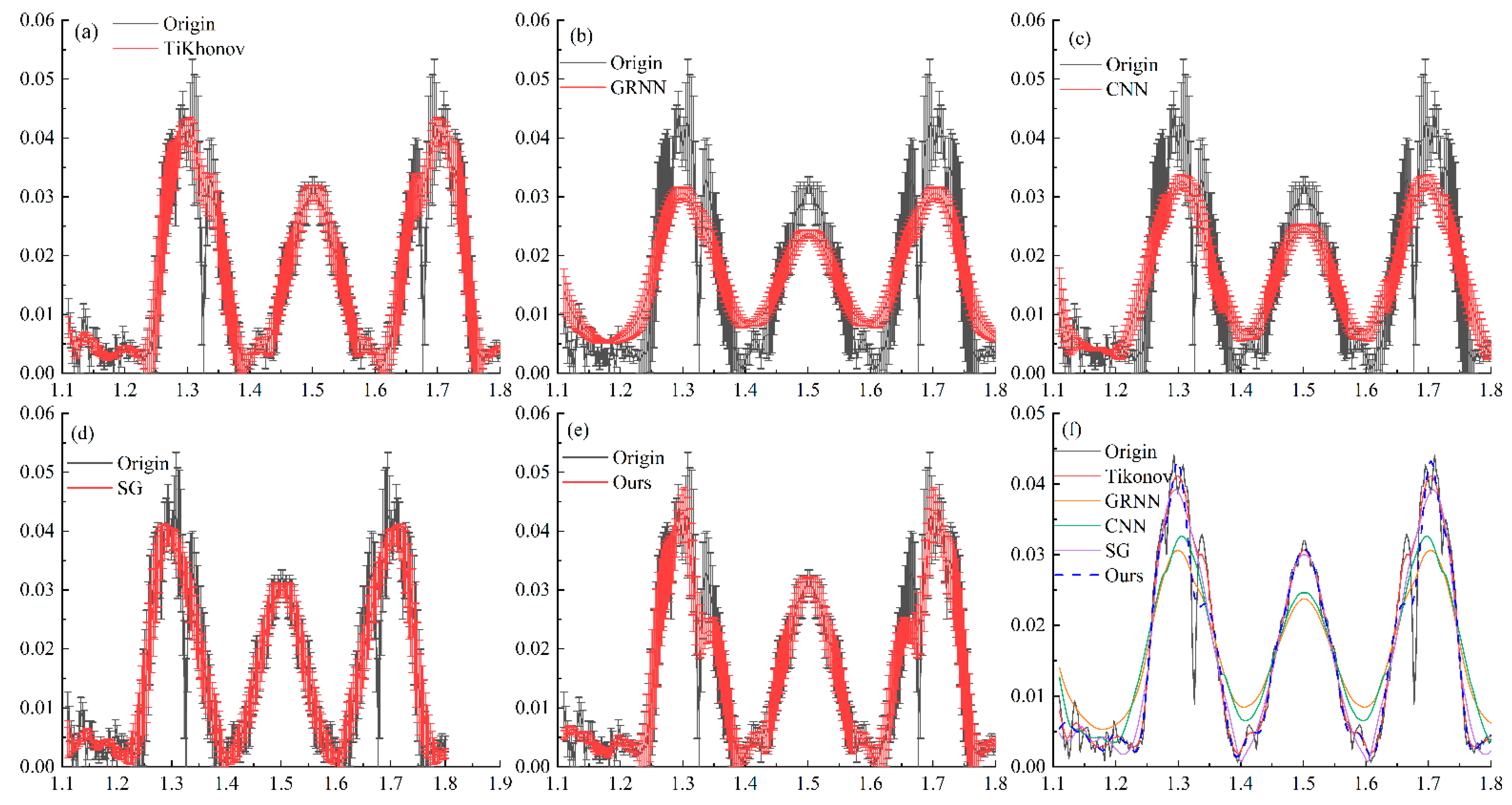
3.4. Real THz Spectrum

The proposed method is applied to remove the noise of the measured signal. In this section, the measured THz spectrum is captured via the system shown in Figure 7. The central wavelength of the femtosecond laser output is 1550 nm, and the lock-in amplifier is applied to remove the background noise and enhance the measured signal. Figure 8 shows the THz denoising effect. Regions A and B of Figure 8 denote the key areas, which comprise the strong and weak peaks, respectively. To evaluate the effect of denoising intuitively, the local enlarged figures of region A and B are shown in Figure 9 and Figure 10, and the error bars, which are calculated from the standard deviation, are also added in Figure 9 and Figure 10.
The restored results by all denoising methods are illustrated in Figure 8, Figure 9 and Figure 10. Figure 9a–e show the magnified view of region A, and Figure 9f shows the denoising effect. Similarly, Figure 10 shows the he magnified view of region B. In the measured spectrum experiment, the signal loss is the universal problem, where the proposed algorithm has the minimum error. For example, all the denoising methods have a low-quality restored effect at the peak valley region (about 0.55 THz) in Figure 10. However, the proposed method has the highest-quality denoising result at 0.55 THz. From Figure 8, the peaks in region B are weak peaks, which is the challenge for denoising. Figure 10 illustrates the effect of preserving weak peaks, and the proposed method can also estimate the high-quality restored spectrum. The performance of CNN based on supervised learning is poor, and two main reasons lead to these situations. First, denoising is an inverse problem, and clean data provided by themselves will have errors; second, the amount of training data also limits the performance of CNN. In addition, the proposed method can estimate the high-quality THz spectrum, but the residual noise and information loss are also the shortcomings of the proposed methods.

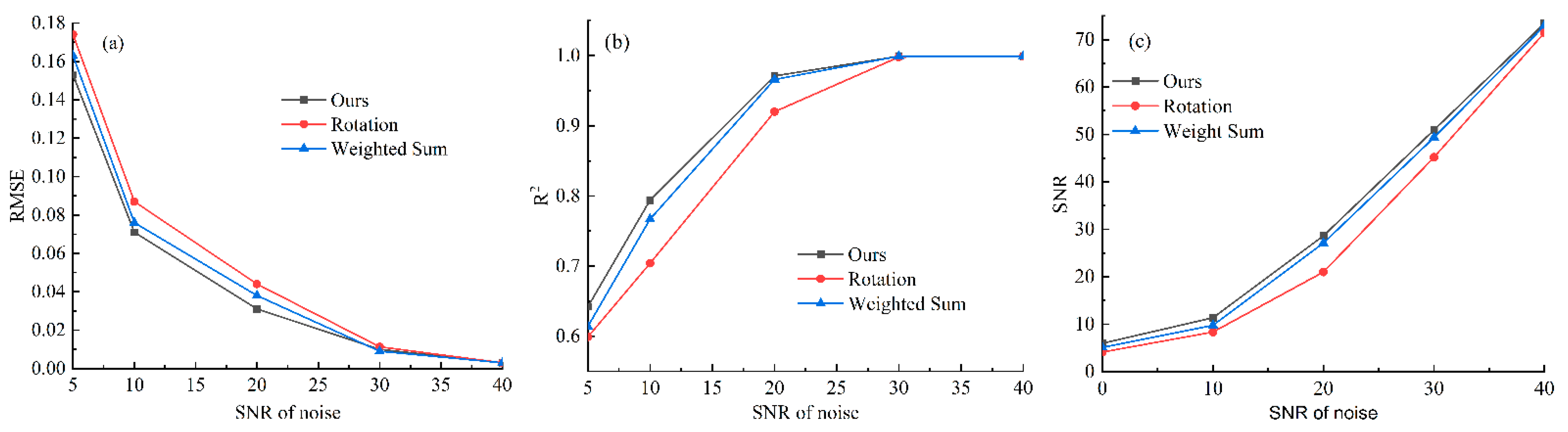
3.5. Data Augmentation Experiment

In this section, the effect of data augmentation by using low-quality underwater images is studied, and we compare it with two useful data experiment methods, including rotation [47] and weighted sum [23], where rotation is a method of image augmentation. To evaluate the result quantitatively, the synthetic spectra of Section 3.3 are applied. For the purpose of impartial evaluation of the performance of the proposed method, the improved Transformer model is adopted as the backbone network. It is worth noting that the rotation operation only inverts the THz spectrum. Figure 11 illustrates the denoising effect for three data augmentation methods.
Figure 11 shows the quantitative analysis for three data augmentation methods. It is seen from Figure 11 that for considered SNR noise levels of 5, 10, 20, 30, and 40 dB, the proposed method obtains the values of RMSE, R2, and SNR, which are superior to other data augmentation methods. From Figure 11, the denoising effect of the rotation operation is poor. From (1), the spectrum peaks are symmetrical; this shows that the rotation operation cannot provide useful information to the neural network, because there is no significant change in spectral peak morphology before and after rotation.

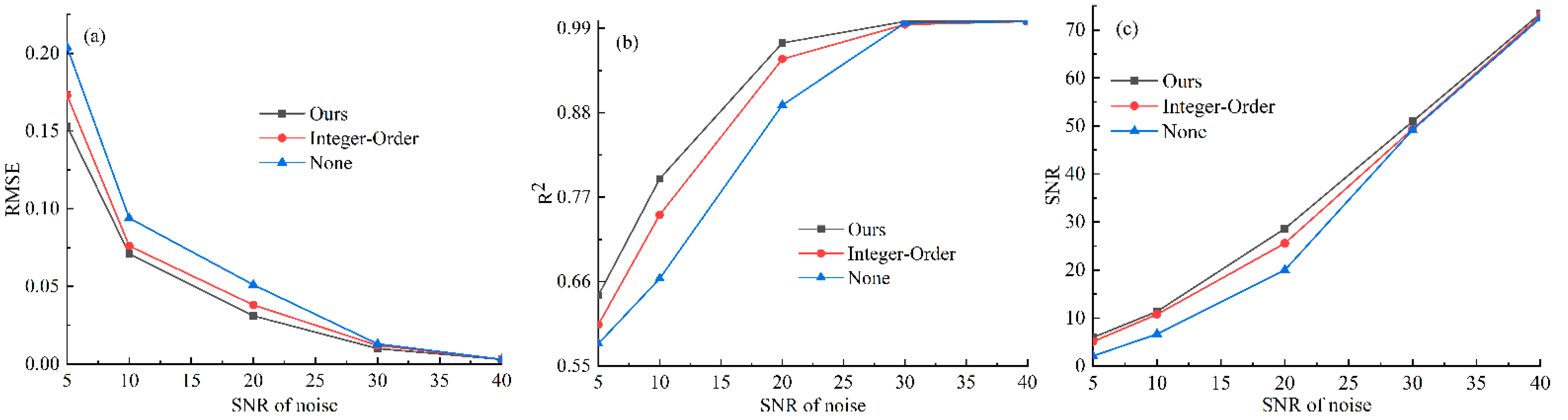
3.6. Fractional-Order Loss Function

In this section, the loss function with fractional-order variation is compared by integer-order and no regularization terms. The process of synthetic spectrum degradation is simulated by using Gaussian noise of 5, 10, 20, 30, and 40 dB SNR noise, where the synthetic spectra are also from Section 3.3. To evaluate the loss function fairly, the proposed Transformer network is used as the backbone network.
The results of different loss functions are shown in Figure 12. When noise levels are low, the effects of several loss functions are similar. When noise levels are high, the fractional-order loss function can estimate the higher-quality spectrum than other loss functions. Due to the synthetic spectrum intensity being less than 1, RMSE and SNR of the above methods are approximate. However, the loss function with no regularization terms has the problem of restoring spectral distortion; this makes the R2 for no regularization terms have a gap compared to other methods.

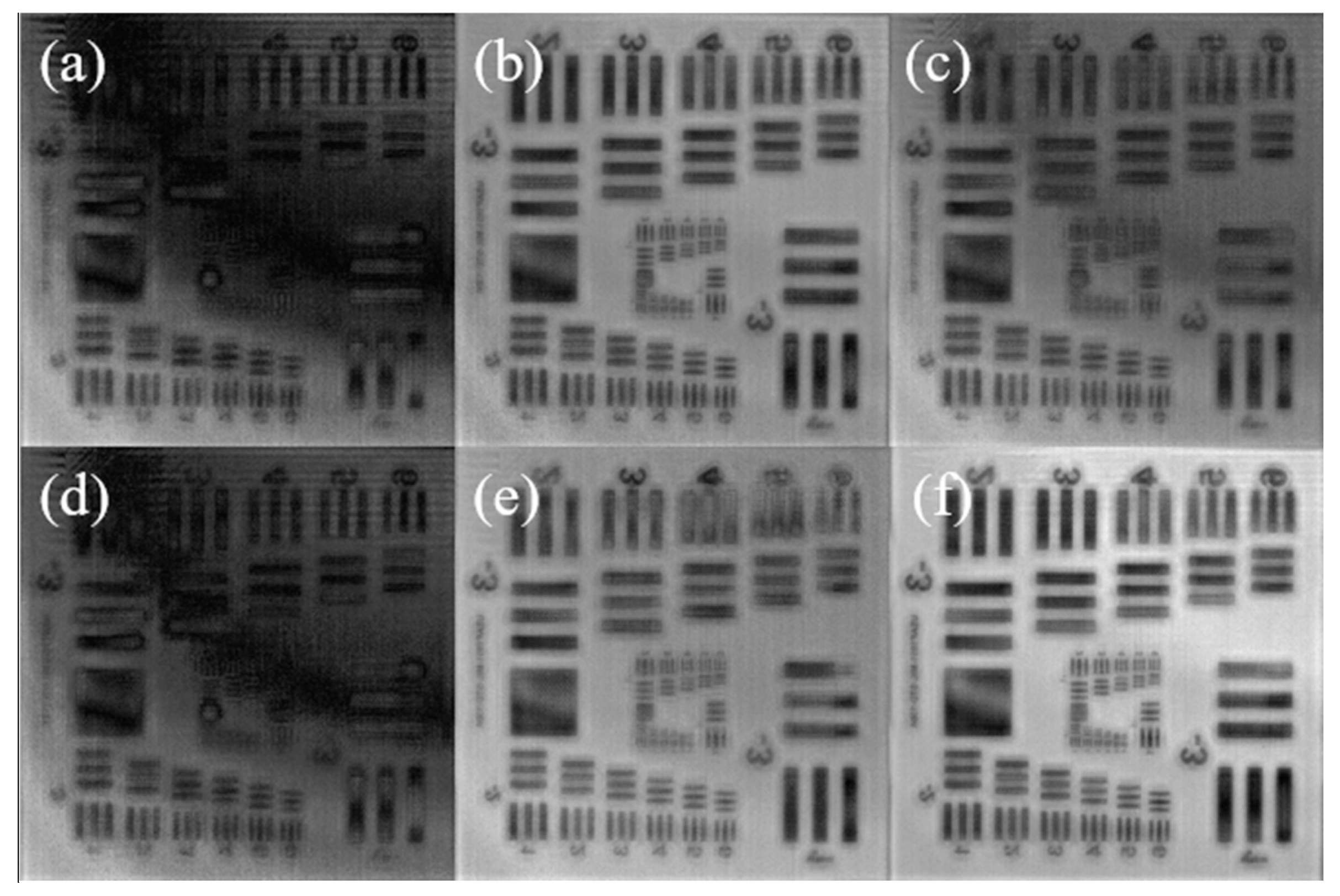
3.7. Application for THz Imaging

In this section, the proposed method is applied to THz imaging to demonstrate its performance. In this section, the experimental data are from [48]. Because the proposed method can remove the 1D spectrum noise, the proposed method only removes noise from the spectral domain without using spatial information to improve imaging quality. For THz imaging, it is difficult to obtain the reference image. Therefore, the no-reference image quality assessment is applied as the merits. In this section, the Blind/Referenceless Image Spatial Quality Evaluator (BRISQUE) [49], and Natural Image Quality Evaluator (NIQE) [50] are the evaluation indexes of the THz image. In addition, to improve the visual quality of the restored THz image, linear stretching is applied. It is worth noting that linear stretching can enhance visual effects and can amplify the noise. Figure 13 shows the restored THz images of channel 10 via spectral denoising methods, and Figure 14 illustrates BRISQUE and NIQE.
From Figure 13, the proposed method can estimate high-quality THz images, and these images have the highest contrast. The original THz image has the phenomenon of information loss. The spectrum denoising methods GRNN and CNN fail to solve this problem. The restored THz images via Tikhonov and SG filter have a better visual effect, but their contrast is lower than the proposed method. Further, the no reference image quality evaluations are applied to compare the restored effect objectively, and the score is shown in Figure 14. From Figure 14, the mean and median of the proposed algorithm are the lowest in BRISQUE and NIQE, and the shortest box indicates that the overall restoration effect of the proposed algorithm is the best denoising method.

4. Conclusions and Prospects

In this paper, a fractional variation THz spectrum denoising network based on Transformer was proposed, which can restore the high-quality THz spectrum without using clean data. The proposed method mainly alleviates four problems. Firstly, to solve the problem that a clean THz spectrum is difficult to obtain, the proposed method is based on the Noise2Noise frame. Secondly, fractional-order variation is applied to improve the L2 loss function, which ameliorates the denoising effect. Thirdly, to remove the noise of the THz spectrum, a Transformer-based network is proposed. Finally, to solve the problem of insufficient THz spectrum data, a low-quality underwater image is used to augment the training data, and this is applied to inhibit the signal offset. Experiments show that the proposed method can estimate the high-quality THz spectrum, and it also has a satisfactory effect on the restoration of THz imaging.
However, the proposed method still has many shortcomings, which can be divided into two categories. Firstly, the common shortcomings of the neural network model include as the fixed input size. The training neural network model has a fixed input size, which improves the importance of size preprocessing of the THz spectrum. In this paper, artificial segmentation is applied to change the size of the THz spectrum, which increases extra work and complexity. Secondly, the disadvantages of the N2N-based method include noise type and loss function. N2N can only remove zero-mean noise, which also limits the practicality of the proposed method. The L2 loss function can lead to data overfitting or poor robustness.
In conclusion, the proposed method can estimate a high-quality THz spectrum without using clean data. The future work will focus on solving problems such as the lack of a low-quality underwater image dataset for terahertz spectrum denoising and a spectral size-changing algorithm.

Author Contributions

All authors contributed substantially to this study. Individual contributions were conceptualization, M.L. and Y.Z.; methodology, Q.J., F.Z. and M.L.; software, Q.J., J.X. and L.K.; validation, Q.J., J.X. and L.D.; formal analysis, Q.J. and F.Z.; investigation, F.Z., M.H. and M.L.; resources, M.L., L.D. and Y.Z.; data curation, Q.J.; writing—original draft preparation, Q.J.; writing—review and editing, Q.J. and J.X.; visualization, Q.J.; supervision, M.L., M.H. and Y.Z.; project administration, M.L.; funding acquisition, M.L. All authors have read and agreed to the published version of the manuscript.

Funding

This research was funded by the National Key Research and Development Project of China (No. 2018YFF0300804), the Graduate Innovation Research Project of the Yangtze Delta Region Academy of the Beijing Institute of Technology, Jiaxing (No. GIIP2021-007, No. GIIP2021-006, No. GIIP2021-011, No. GIIP2021-012), and the National Natural Science Foundation of China (No. 11774031).

Institutional Review Board Statement

This study doesn’t require ethical approval.

Informed Consent Statement

Not applicable.

Data Availability Statement

The publicly archived datasets of the underwater image data used in this paper, are derived from references [42]. The training data are derived from [42,43]. The THz image of Section 3.7 are derived from [48].

Acknowledgments

We would like to thank all the anonymous referees for their constructive comments and suggestions.

Conflicts of Interest

The authors declare that they have no conflict of interest.

References

  1. Ferguson, B.; Zhang, X.C. Materials for terahertz science and technology. Nat. Mater. 2002, 1, 26–33. [Google Scholar] [CrossRef] [PubMed]
  2. Chen, H.T.; Padilla, W.J.; Zide, J.M.O.; Gossard, A.C.; Taylor, A.J.; Averitt, R.D. Active terahertz metamaterial devices. Nature 2006, 444, 597–600. [Google Scholar] [CrossRef] [PubMed] [Green Version]
  3. Zhang, M.J.; Hong, H.C.; Lin, H.J.; Shen, L.G.; Yu, H.Y.; Ma, G.C.; Chen, J.R.; Liao, B.Q. Mechanistic insights into alginate fouling caused by calcium ions based on terahertz time-domain spectra analyses and DFT calculations. Water Res. 2018, 129, 337–346. [Google Scholar] [CrossRef] [PubMed]
  4. Naftaly, M.; Vieweg, N.; Deninger, A. Industrial applications of terahertz sensing: State of play. Sensors 2019, 19, 4203. [Google Scholar] [CrossRef] [Green Version]
  5. Son, J.H.; Oh, S.J.; Cheon, H. Potential clinical applications of terahertz radiation. J. Appl. Phys. 2019, 125, 190901. [Google Scholar] [CrossRef]
  6. Ahmed, K.; Ahmed, F.; Roy, S.; Paul, B.K.; Aktar, M.N.; Vigneswaran, D.; Islam, M.S. Refractive index-based blood components sensing in terahertz spectrum. IEEE Sens. J. 2019, 19, 3368–3375. [Google Scholar] [CrossRef]
  7. Guo, Y.X.; Jin, W.Q.; Guo, Z.Y.; He, Y.Q. Iterative differential autoregressive spectrum estimation for Raman spectrum denoising. J. Raman. Spectrosc. 2022, 531, 148–165. [Google Scholar] [CrossRef]
  8. Naftaly, M. Metrology issues and solutions in THz time-Domain spectroscopy: Noise, errors, calibration. IEEE Sens. J. 2013, 13, 8–17. [Google Scholar] [CrossRef]
  9. Skorobogatiy, M.; Sadasivan, J.; Guerboukha, H. Statistical models for averaging of the pump-probe traces: Example of denoising in terahertz time-domain spectroscopy. IEEE Trans. Terahertz Sci. Technol. 2018, 8, 287–298. [Google Scholar] [CrossRef]
  10. Pupeza, I.; Wilk, R.; Koch, M. Highly accurate optical material parameter determination with THz time-domain spectroscopy. Opt. Express 2007, 15, 4335–4350. [Google Scholar] [CrossRef]
  11. Shen, S.; He, J. SGCS: A signal reconstruction method based on Savitzky-Golaysgz filtering and compressed sensing for wavelength modulation spectroscopy. Opt. Express 2021, 29, 35848–35863. [Google Scholar] [CrossRef] [PubMed]
  12. Khani, M.E.; Arbab, M.H. Chemical identification in the specular and off-specular rough-surface scattered Terahertz spectra using wavelet shrinkage. IEEE Access 2021, 9, 29746–29754. [Google Scholar] [CrossRef] [PubMed]
  13. Zeng, X.X.; Zhang, H.; Xi, X.Q.; Li, B.; Zhou, J. Numerically denoising thermally tunable and thickness-dependent terahertz signals in ErFeO3 based on bézier curves and B-Splines. Ann. Phys. 2021, 533, 2000464. [Google Scholar] [CrossRef]
  14. Wang, S.; Niu, P.J.; Guo, Q.H.; Wang, X.C.; Wang, F.Z. An adaptive empirical mode decomposition and stochastic resonance system in high efficient detection of terahertz radar signal. Ferroelectrics 2020, 536, 148–160. [Google Scholar] [CrossRef]
  15. Liu, H.; Li, Y.; Zhang, Z.; Liu, S.; Liu, T. Blind Poissonian reconstruction algorithm via curvelet regularization for FTIR spectrometer. Opt. Express 2018, 26, 22837–22856. [Google Scholar] [CrossRef]
  16. Chen, X.; Sun, Q.; Stantchev, R.I.; Pickwell-MacPherson, E. Objective and efficient terahertz signal denoising by transfer function reconstruction. APL Photonics 2020, 5, 056104. [Google Scholar] [CrossRef]
  17. Yann, L.C.; Yoshua, B.; Geoffrey, H. Deep learning. Nature 2015, 521, 436–444. [Google Scholar]
  18. Hou, C.P.; Nie, F.P.; Li, X.L.; Yi, D.Y.; Wu, Y. Joint embedding learning and sparse regression: A framework for unsupervised feature selection. IEEE Trans. Cybern. 2014, 44, 793–804. [Google Scholar]
  19. Hui, M.; Wu, Y.; Li, W.; Liu, M.; Dong, L.; Kong, L.; Zhao, Y. Image restoration for synthetic aperture systems with a non-blind deconvolution algorithm via a deep convolutional neural network. Opt. Express 2020, 28, 9929–9943. [Google Scholar] [CrossRef]
  20. Liu, W.; Zhao, Y.; Liu, M.; Yi, W.; Dong, L.; Hui, M. Triple-adjacent-frame generative network for blind video motion deblurring. Neurocomputing 2020, 376, 153–165. [Google Scholar] [CrossRef]
  21. Zhang, K.; Zuo, W.M.; Chen, Y.J.; Meng, D.Y.; Zhang, L. Beyond a Gaussian denoiser: Rresidual learning of deep CNN for image denoising. IEEE Trans. Image Process. 2017, 26, 3142–3155. [Google Scholar] [CrossRef] [PubMed] [Green Version]
  22. Pan, L.; Pipitsunthonsan, P.; Zhang, P.; Daengngam, C.; Booranawong, A.; Chongcheawchamnan, M. Noise reduction technique for Raman spectrum using deep learning network. In Proceedings of the 13th International Symposium on Computational Intelligence and Design, Hangzhou, China, 12–13 December 2020; pp. 159–163. [Google Scholar]
  23. Wahl, J.; Sjödahl, M.; Ramser, K. Single-Step Preprocessing of Raman Spectra Using Convolutional Neural Networks. Appl. Spectrosc. 2020, 74, 427–438. [Google Scholar] [CrossRef] [PubMed]
  24. Jiao, Q.L.; Liu, M.; Yu, K.; Liu, Z.L.; Kong, L.Q.; Hui, M.; Dong, L.Q.; Zhao, Y.J. Spectral Pre-Processing Based on Convolutional Neural Network. Spectrosc. Spectr. Anal. 2022, 42, 292–297. [Google Scholar]
  25. Zhang, Q.; Yang, L.T.; Chen, Z.; Li, P. A survey on deep learning for big data. Inform. Fusion. 2018, 42, 146–157. [Google Scholar] [CrossRef]
  26. Jeong, S.Y.; Cheon, H.; Lee, D.; Son, J.H. Determining terahertz resonant peaks of biomolecules in aqueous environment. Opt. Express 2020, 28, 3854–3863. [Google Scholar] [CrossRef]
  27. Ferrer-Galindo, L.; Sanu-Ginarte, A.D.; Fleitas-Salazar, N.; Ferrer-Moreno, L.A.; Rosas, R.A.; Pedroza-Montero, M.; Riera, R. Denoising and principal component analysis of amplified Raman spectra from red blood cells with added silver nanoparticles. J. Nanomater. 2018, 2018, 9417819. [Google Scholar] [CrossRef]
  28. El Haddad, J.; Bousquet, B.; Canioni, L.; Mounaix, P. Review in terahertz spectral analysis. TrAC-Trend Anal. Chem. 2013, 44, 98–105. [Google Scholar] [CrossRef] [Green Version]
  29. Qiao, L.; Wang, Y.; Zhao, Z.; Chen, Z. Identification and quantitative analysis of chemical compounds based on multiscale linear fitting of terahertz spectra. Opt. Eng. 2014, 53, 074102. [Google Scholar] [CrossRef]
  30. Haslauer, K.; Schmitt-Kopplin, P.; Heinzmann, S. Data processing optimization in untargeted metabolomics of urine using Voigt lineshape model non-linear regression analysis. Metabolites 2021, 11, 285. [Google Scholar] [CrossRef]
  31. Zhuang, F.; Qi, Z.; Duan, K.; Xi, D.; Zhu, Y.; Zhu, H.; Xiong, H.; He, Q. A comprehensive survey on transfer learning. Proc. IEEE 2021, 109, 43–76. [Google Scholar] [CrossRef]
  32. Jiao, Q.; Liu, M.; Li, P.; Dong, L.; Hui, M.; Kong, L.; Zhao, Y. Underwater image restoration via non-convex non-smooth variation and thermal exchange optimization. J. Mar. Sci. Eng. 2021, 9, 570. [Google Scholar] [CrossRef]
  33. Jaakko, L.; Jacob, M.; Jon, H.; Samuli, L.; Tero, K.; Miika, A.; Timo, A. Noise2Noise: Learning Image Restoration without Clean Data. arXiv 2018, arXiv:1803.04189. [Google Scholar]
  34. Zhang, X.; Li, D.Q.; Li, J.; Liu, B.; Jiang, Q.Y.; Wang, J.H. Signal-Noise Identification for Wide Field Electromagnetic Method Data Using Multi-Domain Features and IGWO-SVM. Fractal Fract. 2022, 6, 80. [Google Scholar] [CrossRef]
  35. Stoica, R.-A.; Iimori, H.; de Abreu, G.T.F.; Ishibashi, K. Frame Theory and Fractional Programming for Sparse Recovery-Based mmWave Channel Estimation. IEEE Access 2019, 7, 150757–150774. [Google Scholar] [CrossRef]
  36. Yang, Q.; Chen, D.; Zhao, T.; Chen, Y. Fractional Calculus in Image Processing: A Review. Fract. Calc. Appl. Anal. 2016, 19, 1222–1249. [Google Scholar] [CrossRef] [Green Version]
  37. Zhang, X.; Dai, L. Image Enhancement Based on Rough Set and Fractional Order Differentiator. Fractal Fract. 2022, 6, 212. [Google Scholar] [CrossRef]
  38. Vaswani, A.; Shazeer, N.; Parmar, N.; Uszkoreit, J.; Jones, L.; Gomez, A.N.; Kaiser, L.; Polosukhin, I. Attention Is All You Need. arXiv 2017, arXiv:1706.03762. [Google Scholar]
  39. Fan, H.; Xiong, B.; Mangalam, K.; Li, Y.; Yan, Z.; Malik, J.; Feichtenhofer, C. Multiscale Vision Transformers. arXiv 2021, arXiv:2104.11227. [Google Scholar]
  40. Hou, Y.; Xu, J.; Liu, M.; Liu, G.; Liu, L.; Zhu, F.; Shao, L. NLH: A Blind Pixel-Level Non-Local Method for Real-World Image Denoising. IEEE Trans. Image Process. 2020, 29, 5121–5135. [Google Scholar] [CrossRef] [Green Version]
  41. Yu, K.; Cheng, Y.F.; Li, L.F.; Zhang, K.H.; Liu, Y.L.; Liu, Y.F. Underwater Image Restoration via DCP and Yin–Yang Pair Optimization. J. Mar. Sci. Eng. 2022, 10, 360. [Google Scholar] [CrossRef]
  42. Linstrom, P.J.; Mallard, W.G. NIST Chemistry WebBook, NIST Standard Reference Database Number 69; National Institute of Standards and Testing (NIST): Gaithersburg, MD, USA, 2013. [Google Scholar]
  43. Available online: https://figshare.com/ (accessed on 26 June 2019).
  44. Liu, H.; Zhang, Z.L.; Liu, S.Y.; Yan, L.X.; Liu, T.T.; Zhang, T.X. Joint Baseline-Correction and Denoising for Raman Spectra. Appl. Spectrosc. 2015, 69, 1013–1022. [Google Scholar] [CrossRef] [PubMed]
  45. Djarfour, N.; Ferahtia, J.; Babaia, F.; Baddari, K.; Said, E.; Farfour, M. Seismic noise filtering based on Generalized Regression Neural Networks. Comput. Geosci. 2014, 69, 1–9. [Google Scholar] [CrossRef]
  46. Sun, X.; Liu, J.; Zhu, K.; Hu, J.; Jiang, X.; Liu, Y. Generalized regression neural network association with terahertz spectroscopy for quantitative analysis of benzoic acid additive in wheat flour. R. Soc. Open Sci. 2019, 7, 190485. [Google Scholar] [CrossRef] [PubMed] [Green Version]
  47. Cheng, G.; Zhou, P.; Han, J. Learning Rotation-Invariant Convolutional Neural Networks for Object Detection in VHR Optical Remote Sensing Images. IEEE Trans. Geosci. Remote Sens. 2016, 54, 7405–7415. [Google Scholar] [CrossRef]
  48. Wong, T.M.; Kahl, M.; Bolívar, P.H.; Kolb, A.; Möller, M. Training Auto-enconder-Based Optimizers for Terahertz Image Reconstruction. In Proceedings of the 2019 German Conference on Pattern Recognition, Dortmund, Germany, 10–13 September 2019; pp. 93–106. [Google Scholar]
  49. Mittal, A.; Moorthy, A.K.; Bovik, A. No-Reference Image Quality Assessment in the Spatial Domain. IEEE Trans. Image Process. 2012, 21, 4695–4708. [Google Scholar] [CrossRef] [PubMed]
  50. Mittal, A.; Rajiv, S.; Bovik, A.C. Making a “Completely Blind” Image Quality Analyzer. IEEE Signal Proc. Lett. 2012, 20, 209–212. [Google Scholar] [CrossRef]
Figure 1. Comparison of the traditional and proposed methods.
Fractalfract 06 00246 g001
Figure 2. (a) The principle of underwater imaging. (b) Comparison of THz spectrum with the row pixel intensity of underwater images.
Fractalfract 06 00246 g002
Figure 3. The architecture of the Transformer and its modules. (a) The architecture of the Transformer. (b) The architecture of the encoder. (c) The architecture of MLP. (d) The architecture of MSA. (e) The principle of scaled dot-product attention.
Fractalfract 06 00246 g003
Figure 4. The architecture of the improved Transformer.
Fractalfract 06 00246 g004
Figure 5. The quantitative analysis results of the synthesized spectrum. (a) The score of RMSE, (b) The score of R2. (c) The score of SNR.
Fractalfract 06 00246 g005
Figure 6. The denoising effect. (a) The noisy synthetic spectra. (bf) Comparison of synthetic spectra with Tikhonov, GRNN, CNN, SG, and the proposed method, respectively.
Fractalfract 06 00246 g006
Figure 7. The experimental system.
Fractalfract 06 00246 g007
Figure 8. The real THz spectrum experiment. Region A and B are enlarged in Figure 9 and Figure 10.
Fractalfract 06 00246 g008
Figure 9. The restored effect of region A. (ae) Comparison of real THz spectra with Tikhonov, GRNN, CNN, SG, and the proposed method, respectively. The error bars are calculated from the standard deviation. (f) The denoising effect without error bars.
Fractalfract 06 00246 g009
Figure 10. The restored effect of region B. (ae) Comparison of real THz spectra with Tikhonov, GRNN, CNN, SG, and the proposed method, respectively. The error bars are calculated from the standard deviation. (f) The denoising effect without error bars.
Fractalfract 06 00246 g010
Figure 11. The quantitative denoising result with different data augmentation methods. (a) RMSE; (b) R2; (c) SNR.
Fractalfract 06 00246 g011
Figure 12. The quantitative denoising result with loss functions of fractional-order, integer-order, and no regularization terms. (a) RMSE. (b) R2. (c) SNR.
Fractalfract 06 00246 g012
Figure 13. The restored THz imaging. (a) The original image of channel 10; (bf) the restored THz image via Tikhonov, GRNN, CNN, SG filter, and the proposed method.
Fractalfract 06 00246 g013
Figure 14. The no reference image quality evaluation score. (a) The BRISQUE score. (b) The NIQE score.
Fractalfract 06 00246 g014
Table 1. Similarity between images and THz spectrum.
SSIMAbsolute Value of R2p (α = 0.05)
MeanMedianMeanMedianMeanMedian
Underwater images0.36970.37530.27640.23300.0344<0.0001
Natural images0.33440.35780.23850.19610.0665<0.0001
Nighttime images0.27130.25330.18940.16270.0354<0.0001
Table 2. The restored effect of images (the noise is 10 dB).
R2RMSESNR/dB
Underwater images0.7940.07113.125
Natural images0.6310.1379.644
Nighttime images0.7590.08311.739
Table 3. The quantitative analysis of restored THz spectrum peaks.
Peak ID StandardTikhonovGRNNCNNSGOurs
1Position3535.234.435.434.234.6
Intensity0.70.7070.67130.6930.6890.697
2Position797879.677.879.279
Intensity0.6160.4950.5070.3980.5680.620
3Position90.693.289.684.293.290.2
Intensity0.8740.5180.6350.4100.4190.873
4Position108108.4107.8108.2108.2108
Intensity0.860.8630.8330.8510.8530.861
5Position185184.6186.6184.8184.4184.8
Intensity0.710.7050.6860.6980.6990.708
Publisher’s Note: MDPI stays neutral with regard to jurisdictional claims in published maps and institutional affiliations.

