Results on Neutral Partial Integrodifferential Equations Using Monch-Krasnosel’Skii Fixed Point Theorem with Nonlocal Conditions

Abstract

In this theory, the existence of a mild solution for a neutral partial integrodifferential nonlocal system with finite delay is presented and proved using the techniques of the Monch–Krasnosel’skii type of fixed point theorem, a measure of noncompactness and resolvent operator theory. For this work, we have introduced some sufficient conditions to confirm the existence of the neutral partial integrodifferential system. An illustration of the derived results is offered at the end with a filter system corresponding to our existence result.

1. Introduction

We establish the solution of the existence of Equations (1) and (2) with finite delay

$$\begin{array}{c}\frac{d}{dv}\mathcal{D}(v,z_v)=\mathbb{A}\mathcal{D}(v,z_v)+{\int }_0^{v}H(v-s)\mathcal{D}(s,z_s)ds\hfill \\ \hfill +\varphi \left(v,z_v,{\int }_0^{v}h(v,s,z_s)ds\right),\mathrm{for}v\in I=[0,b],& \end{array}$$

(1)

$$\begin{array}{cc}\hfill & z_0=\phi +g\left(z\right)=C([-r,0];X).\end{array}$$

(2)

Here, $\mathbb{A}$ is a closed linear operator defined on Banach space $(X,\parallel ·\parallel )$ with domain $D\left(\mathbb{A}\right)$. Let ${\left[H\left(v\right)\right]}_{v\ge 0}$ be the set of all closed linear operators on X with domain $D\left(H\right)\supset D\left(\mathbb{A}\right)$ and $C\left(\right[-r,0];X)$ denote the set of all continuous functions defined on $[-r,0]$ into X. Throughout this theory, X will be used as Banach space. The function $\mathcal{D}$ in ${\mathbb{R}}^{+}\times C\to X$ is defined as follows

$$\begin{array}{cc}\hfill & \mathcal{D}(v,\phi )=\phi \left(0\right)-F(v,\phi ),\hfill \end{array}$$

where the function F is continuous from ${\mathbb{R}}^{+}\times C$ into X and the function $\varphi$ is also continuous from ${\mathbb{R}}^{+}\times C\times X$ into X. Let $z\in C\left([-r,0];X\right)$, $\forall v\ge 0$, then the history function $z_v\in C$ is defined by

$$\begin{array}{cc}\hfill & z_v\left(t\right)=z(v+t)\mathrm{for}t\in [-r,0].\hfill \end{array}$$

Semigroup theory provides a unified and powerful tool for the study of differential equations on Banach space-covering systems described by ordinary differential equations, functional differential equations, partial differential equations, and neutral differential equations, etc. In recent years, among many other applications, semigroup theory has been widely used in the study of control and stability of systems governed by differential equations on Banach space. It has been discussed by many authors for $\mathbb{A}$ is densely defined. In [1,2], the authors studied the hypotheses for the existence of resolvent operators for the abstract integrodifferential equations. Further, in [3,4,5,6,7], the authors discussed the solutions of the existence of nonlinear neutral partial differential equations using different approaches. Lizama et al. [8] studied (1) with the nonlocal initial values when $\varphi =0$, and using the fixed point of Sadovskii’s technique, derived the solution of existence when the nonlocal condition is compact, and $R_1(·)$ is continuous with respect to the norm. Many authors have proven the existence of the solution for neutral integrodifferential equations with initial and nonlocal conditions. In [9], the authors proved the solutions of neutral functional integrodifferential equations with an initial condition in finite delay, and in [4], the authors proved the existence of the mild solution for a class of neutral partial integrodifferential equations using resolvent operator theory and measure of noncompactness and proved the existence using the Monch–Krasnosel’skii type of fixed point theorem with initial conditions. Motivated by the above two particular articles, we construct a new problem (1) and (2) using nonlocal conditions with finite delay and apply the Monch–Krasnosel’skii fixed point technique. The contribution of this article is extended from the neutral integrodifferential equation, including an integral term in functional and taking nonlocal conditions with finite delay. As is well-known, the nonlocal problems are more desirable when compared with Cauchy problems. In considerations with real-life phenomena, generally, the physical changes of a system depend on both its present and past states. In order to face certain situations, nonlocal conditions play a vital role. Many problems in the field of ordinary and partial differential equations can be recast as integral equations. Several existence and uniqueness results can be derived from the corresponding results of integral equations. The fixed point method is the most powerful method in proving existence theorems for integrodifferential equations. This paper consists of Section 2, to provide basic lemmas and results to use in this article. In Section 3, we provide some results from the new Monch–Krasnosel’skii type of fixed point theorem. In Section 4, we derive the mild solution of (1) and (2) and discuss the existence result. Section 5 gives an application to validate our theory, and Section 6 gives a filter system corresponding to the solution of existence in our differential system. Finally in Section 7, we provide the conclusion about this article.

2. Results on Measure of Noncompactness

Here, we define some useful definitions and lemmas to use in this analysis. Let $\mathcal{C}\left(\right[0,b];X)$ be the set of all continuous functions defined on $[0,b]$ in X with a standard supreme norm. For Banach spaces Z and W, we denote by $\mathcal{L}(Z,W)$ the Banach space of all bounded linear operators from Z into W. The Banach space X with graph norm is declared as ${∥x∥}_G={∥\mathbb{A}x∥}_X+{∥x∥}_X$ and denoted by $(Y,\parallel ·\parallel )$. For this theory, we need the following results about the resolvent operator theory, see [1,2]. Consider the following integrodifferential equation

$$\begin{array}{cc}\hfill & u^{\prime }\left(t_1\right)=Au\left(t_1\right)+{\int }_0^{t_1}B(t_1-s)u\left(s\right)ds,t_1\ge 0,u\left(0\right)=u_0\in X.\hfill \end{array}$$

(3)

Assume that

 (P1)

A is a closed linear operator and densely defined on Banach space $(X,\parallel ·\parallel )$ with graph norm $\parallel x\parallel =\parallel Ax\parallel +\parallel x\parallel$, which is denoted as $(Y,∥·∥)$.

 (P2)

${\left[B\left(t_1\right)\right]}_{t_1\ge 0}$ be the set of all linear operators on X and $B\left(t_1\right)$ is continuous for $t_1\ge 0$, there is a positive real-valued function b such that $\parallel B\left(t_1\right)\left(y\right){\parallel }_X\le b\left(t_1\right){∥y∥}_G$, $\forall y\in Y$, $t_1\ge 0$.

 (P3)

For any $y\in Y$, then $t_1\to B\left(t_1\right)y\in W_{loc}^{1,1}({\mathbb{R}}^{+},X)$ and $|\frac{d}{d{t}_1}B\left(t_1\right)y|\le b\left(t_1\right)∥y∥$, $\forall t_1\in {\mathbb{R}}^{+}$.

Definition 1.

Let $R_1\left(t_1\right)\in \mathcal{L}\left(X\right)$ be a bound linear operator for $t_1\ge 0$ and a resolvent operator for (3); then, it satisfies

 (i)

$R_1\left(0\right)=I$ and $\parallel R_1\left(t_1\right){\parallel }_{\mathcal{L}}\le M{e}^{\beta t_1}$, where M, β are constants.

 (ii)

$R_1\left(t_1\right)x$ is strongly continuous, $\forall x\in X$ and $t_1\ge 0$.

 (iii)

$R_1\left(t_1\right)\in \mathcal{L}\left(X\right)$, $t_1\ge 0$ and let $x\in Y$ such that $R_1(·)x$ in both $C^1\left({\mathbb{R}}^{+},X\right)$ and $C\left({\mathbb{R}}^{+},X\right)$ and

$$\begin{array}{ccc}\hfill R_1^{\prime }\left(t_1\right)x& =& A{R}_1\left(t_1\right)x+{\int }_0^{t_1}B(t_1-s)R_1\left(s\right)xds\hfill \\ & =& R_1\left(t_1\right)Ax+{\int }_0^{t_1}{R}_1(t_1-s)B\left(S\right)xds,\mathrm{for}{t}_1\ge 0.\hfill \end{array}$$

Theorem 1.

Suppose that $\left(P1\right)$ to $\left(P3\right)$ hold. Then problem (3) admits the resolvent operator if and only if A generates a $C_0$-semigroup.

Lemma 1.

Let S be a bounded subset of X and let ϕ be a function defined on S called the measure of noncompactness (MNC), such that

(1)

$\varphi \left(S\right)=0$ if and only if S is relatively compact.

(2)

$\varphi \left(S\right)=\varphi \left(\overline{S}\right)=\varphi \left(\overline{co}\left(S\right)\right)$, where $\overline{co}\left(S\right)$ is the convex closed hull of S.

(3)

A MNC is called full, if $\varphi \left(S\right)=0$ if and only if S is relatively compact.

(4)

A MNC is monotone if the sets $S_1$ and $S_2$ of X are $S_1\subset S_2\Rightarrow \varphi \left(S_1\right)\le \varphi \left(S_2\right).$

(5)

A MNC is non-singular if $\varphi (S\cup \left\{x\right\})=\varphi \left(S\right)$ for some $S\subseteq X$ and $x\in X$.

Now we define the Hausdorff measure:

$\psi \left(S\right)=inf\left\{r>0;\mathit{where}S\mathit{has}a\mathit{number}\mathit{of}\mathit{sets}\mathit{that}\mathit{covers}S\mathit{with}\mathit{diameter}\le r\right\}$.

Here, the Hausdorff measure is full, monotone and non-singular.

Lemma 2

([10]). Let $S_1$ and $S_2$ be bounded subsets of X, then the following properties are satisfied

 (i)

$\psi \left(S_1+S_2\right)\le \psi \left(S_1\right)+\psi \left(S_2\right)$.

 (ii)

$\psi \left(\lambda S\right)=\left|\lambda \right|\psi \left(S\right)$ where λ is real number.

 (iii)

If ${\left(S_n\right)}_n$ is a decreasing bounded sequence of X with $\underset{n\to \infty }{lim}\psi \left(S_n\right)=0$, then $\underset{n=0}{\overset{\infty }{\cap }}{S}_n$ is a compact set in X.

 (iv)

The map $B:X\to X$ is Lipschitz continuous with a constant k such that $\psi \left(B\left(S\right)\right)\le k\psi \left(S\right)$ for some bounded subset S of X.

For this connection, $\mathcal{C}(I,X)$ is continuous and functions on $I=[0,b]$ in X and supreme norm defined by $\parallel X_{\infty }\parallel =sup\left\{\parallel X\left(t_1\right){\parallel }_X;t_1\in I\right\}$.

From ([11], p. 273), let M be a closed convex subset of X and $\mathcal{K}$ and $\mathcal{S}$ be two nonlinear mappings from M to X. For some ${\Omega }_0\subseteq M$ and $x_0\in X$, we define

$$\begin{array}{ccc}\hfill \mathit{F}\left(\mathcal{K},\mathcal{S},{\Omega }_{\mathit{0}}\right)& =& \left\{x=\mathcal{S}x+\mathcal{K}y\Rightarrow x\in M,\mathit{for}\mathit{any}y\in {\Omega }_0\right\}\hfill \\ \hfill {\mathit{F}}^{(\mathit{1},{\mathit{x}}_{\mathit{0}})}\left(\mathcal{K},\mathcal{S},{\Omega }_{\mathit{0}}\right)& =& \overline{co}\left(\left\{x_0\right\}\cup \mathit{F}\left(\mathcal{K},\mathcal{S},{\Omega }_{\mathit{0}}\right)\right)\hfill \\ \hfill {\mathit{F}}^{({\mathit{n}}_{\mathit{0}},{\mathit{x}}_{\mathit{0}})}\left(\mathcal{K},\mathcal{S},{\Omega }_{\mathit{0}}\right)& =& \overline{co}\left(\left\{x_0\right\}\cup \mathit{F}\left(\mathcal{K},\mathcal{S}\left({\mathit{F}}^{(\mathit{n}-\mathit{1},{\mathit{x}}_{\mathit{0}})}\left(\mathcal{K},\mathcal{S},{\Omega }_{\mathit{0}}\right)\right)\right)\right),n>1.\hfill \end{array}$$

Here, all the sets $\mathit{F}\left(\mathcal{K},\mathcal{S},{\Omega }_{\mathit{0}}\right)$ are nonempty, because if $\mathcal{S}=0$ then ${\mathit{F}}^{({\mathit{n}}_{\mathit{0}},{\mathit{x}}_{\mathit{0}})}\left(\mathcal{K},\mathit{0},{\Omega }_{\mathit{0}}\right)$ reduces to $\mathit{F}\left(\mathcal{K},{\Omega }_{\mathit{0}}\right)$. In this case, $\mathit{F}\left(\mathcal{K},\mathcal{S},{\Omega }_{\mathit{0}}\right)$ is maybe empty. Therefore, it is difficult to find a fixed point for the sum $\mathcal{S}+\mathcal{K}$ in ${\Omega }_{\mathit{0}}$. Therefore, $\mathit{F}\left(\mathcal{K},\mathcal{S},{\Omega }_{\mathit{0}}\right)$ must be nonempty.

Lemma 3

([11]). Let M be a closed convex nonempty subset of X. Then

 (a)

$\mathcal{S}$ is a strict contradiction of X into itself with constant k in $(0,1)$.

 (b)

$x=\mathcal{S}x+\mathcal{K}y\Rightarrow x\in M$ for some $y\in M$.

Then

 (i)

${\mathit{F}}^{({\mathit{n}}_{\mathit{0}},{\mathit{x}}_{\mathit{0}})}\left(\mathcal{K},\mathcal{S},{\Omega }_{\mathit{0}}\right)\subseteq \mathit{M}$ is a nonempty set, for some ${\Omega }_0\subset M$, $n\ge 1$.

 (ii)

${\mathit{F}}^{({\mathit{n}}_{\mathit{0}},{\mathit{x}}_{\mathit{0}})}\left(\mathcal{K},\mathcal{S},{\Omega }_{\mathit{0}}\right)={\mathit{F}}^{({\mathit{n}}_{\mathit{0}},{\mathit{x}}_{\mathit{0}})}\left({(\mathit{I}-\mathcal{S})}^{-\mathit{1}}\mathcal{K},{\Omega }_{\mathit{0}}\right)$for${\Omega }_0\subset M$, $n\ge 1$.

 (iii)

${\Omega }_1\subset {\Omega }_2\subset M$ implies ${\mathit{F}}^{({\mathit{n}}_{\mathit{0}},{\mathit{x}}_{\mathit{0}})}\left(\mathcal{K},\mathcal{S},{\Omega }_1\right)\subset {\mathit{F}}^{({\mathit{n}}_{\mathit{0}},{\mathit{x}}_{\mathit{0}})}\left(\mathcal{K},\mathcal{S},{\Omega }_2\right)\subset \mathit{M}$ for any $n\ge 1$.

Lemma 4

([12]). Let $H:[0,b]\to X$ be an equicontinuous map and $x_0\in [0,b]$, then $\overline{co}\left(H\cup \left\{x_0\right\}\right)$ is also equicontinuous.

Lemma 5

([10]). Let H be a bounded subset of $\mathcal{C}\left([0,b],X\right)$ and for some $t_1\in [0,b]$ such that $\psi \left(H\left(t_1\right)\right)\le {\psi }_c\left(H\right)$, where $H\left(t_1\right)=\left\{x\left(t_1\right);x\in H\right\}$. Moreover, if H is equicontinuous on $[0,b]$, it implies that $t_1\to \psi \left(H\left(t_1\right)\right)$ is continuous on $[0,b]$, ${\psi }_c\left(H\right)={\psi }_{\infty }\left(H\right),$ and

${\psi }_{\infty }\left(H\right)=sup\left\{\psi \left(H\left(t_1\right)\right);t_1\in [0,b]\right\}$.

Lemma 6

([13]). Let H be a bounded subset of X, if there is $\left(u_n\right)$ in H, then

$$\begin{array}{c}\hfill \psi \left(H\right)=\psi \left(u_n\right)\mathit{for}n\ge 1.\end{array}$$

Lemma 7

([14]). Let $0<ϵ<1$, $h>0$ and denote $C_n^m=\left({}_m^n\right)$ for all $0\le m\le n$ such that

$$\begin{array}{c}\hfill S_n={ϵ}^n+C_n^1{ϵ}^{n-1}\frac{h^1}{1!}+C_n^2{ϵ}^{n-2}\frac{h^2}{2!}+....+\frac{h^n}{n!},n\in \mathbb{N}.\end{array}$$

Then $\underset{n\to \infty }{lim}{S}_n=0$.

3. Important Results on Fixed Point Theorem

Here, we provide some results based on a new fixed point technique.

Lemma 8.

Let $\mathcal{S}$ be a contraction map on $X\to X$ with constant k in $[0,1)$, then ${\left(I-\mathcal{S}\right)}^{-1}$ is a continuous map from X into itself with a lipschitzian constant $\frac{1}{1-k}$.

Theorem 2.

Let M be a nonempty closed convex subset of X. Let $\mathcal{K}:M\to X$ and $\mathcal{S}:X\to X$ be two continuous mappings satisfying the following axioms

 (i)

There exist $x_0\in M$ and $n_0>0$ such that for all countable subsets $C\subset M$, we have

$\overline{C}={\mathit{F}}^{({\mathit{n}}_{\mathit{0}},{\mathit{x}}_{\mathit{0}})}\left(\mathcal{K},\mathcal{S},\mathit{C}\right)$, which implies that C is relatively compact.

 (ii)

The mapping $\mathcal{S}$ is a strict contraction.

 (iii)

$x=\mathcal{S}x+\mathcal{K}y$, for some y in $M\Rightarrow x\in M$.

Then, $\mathcal{K}+\mathcal{S}$ has a fixed point in M.

Corollary 1.

Let M be a nonempty closed convex subset of X and ϕ be a non-singular measure of noncompactness on X. Let $\mathcal{K}:M\to X$ and $\mathcal{S}:X\to X$ be two continuous mappings. Then

 (i)

Let $\Omega \subseteq X$ be a countable set with $\varphi (\Omega )>0$ such that

$$\begin{array}{cc}\hfill & \varphi \left({\mathit{F}}^{({\mathit{n}}_{\mathit{0}},{\mathit{x}}_{\mathit{0}})}\left(\mathcal{K},\mathcal{S},\Omega \right)\right)<\varphi \left(\Omega \right)\mathit{for}\mathit{some}{x}_0\in M,n_0>0.\hfill \end{array}$$

(4)

 (ii)

The mapping $\mathcal{S}$ is a strict contraction.

 (iii)

If $x=\mathcal{S}x+\mathcal{K}y$, for some y in $M\Rightarrow x\in M.$ Then $\mathcal{K}+\mathcal{S}$ has a fixed point in M.

Corollary 2

([15]). Let M be a nonempty closed convex subset of X and ϕ be a measure of noncompactness on X. Let $\mathcal{K}:M\to X$ be a continuous map and let $\Omega \subseteq M$ be countable with $\varphi (\Omega )>0$ such that

$$\begin{array}{cc}\hfill & \varphi \left(\mathcal{K}\left(\Omega \right)\right)<\varphi \left(\Omega \right),\hfill \end{array}$$

(5)

then $\mathcal{K}$ has a fixed point in M.

4. Results on Existence

Here, to establish the result on the existence of (1) and (2), we need the following results and lemmas.

Theorem 3.

The continuous function $\mathit{F}$ from $[0,\infty )$ to $\mathcal{L}\left(X\right)$ and for some compact set $K\subset X$, then

$$\begin{array}{c}\hfill \underset{y\in K}{sup}\parallel \mathit{F}\left(\mathit{v}\right)\mathit{y}-\mathit{F}\left({\mathit{v}}_{\mathit{0}}\right)\mathit{y}\parallel \to \mathit{0}\mathrm{as}\mathit{v}\to {\mathit{v}}_{\mathit{0}}.\end{array}$$

The operator V defined on $L^1([0,b];X)$ in $\mathcal{C}\left(\right[0,b];X)$ satisfies,

(S1)

For some $d>0$, we have

$$\begin{array}{c}\hfill \parallel V{f}_1\left(v\right)-V{f}_2{\left(v\right)\parallel }_X\le d{\int }_0^v{\parallel f_1\left(s\right)-f_2\left(s\right)\parallel }_{X}ds,\mathrm{for}\mathrm{all}{f}_1,f_2\in L^1([0,b];X),v\in [0,b].\end{array}$$

(S2)

The compact set $K\subset X$ and ${\left(f_n\right)}_{n\ge 1}\subset L^1([0,b];X)$ implies ${\left(f_n\left(v\right)\right)}_{n\ge 1}\subset K$ for all $v\in [0,b]$ we have

$$\begin{array}{c}\hfill f_n\to f_0\Rightarrow V{f}_n\to V{f}_0.\end{array}$$

Theorem 4

([16]). Suppose the operator V satisfies $\left(S_1\right)$ and $\left(S_2\right)$ and ${\left(f_n\right)}_{n\ge 1}\subset L^1([0,b];X)$ is integrable and bounded,

$$\begin{array}{cc}\hfill & \parallel f_n\left(v\right)\parallel \le \omega \left(v\right),\forall v\in [0,b],n\ge 1,\mathrm{for}\mathrm{some}\omega \in L^1(0,b).\hfill \end{array}$$

Assume that for all $v\in [0,b]$ and for some $q\in L^1(0,b)$ such that

$$\begin{array}{cc}\hfill & \psi \left({\left(f_n\left(v\right)\right)}_{n\ge 1}\right)\le q\left(v\right).\hfill \end{array}$$

Then

$$\begin{array}{c}\hfill \psi \left({\left(V{f}_n\left(v\right)\right)}_{n\ge 1}\right)\le 2d{\int }_0^{v}q\left(s\right)ds\mathrm{for}\mathrm{all}v\in [0,b],d\in S_1.\end{array}$$

Definition 2.

The continuous function $z:[-r,\infty )\to X$ is called a mild solution of Equations (1) and (2) if the following integral equation is satisfied,

$$\begin{array}{cc}z\left(v\right)=F(v,z_v)+R_1\left(v\right)\left[\mathcal{D}\left(0,\phi \left(0\right)+g\left(z\right)\left(0\right)\right)\right]\hfill & \\ \\ +{\int }_0^v{R}_1(v-s)\varphi \left(s,z_s,{\int }_0^{s}h(s,\tau ,z_{\tau })d\tau \right)ds.\hfill \end{array}$$

(6)

To establish this result, we need the below hypotheses:

(H1)

The mapping $\varphi :[0,b]\times C\times X$ satisfied Caratheodary conditions, i.e., $\varphi (v,·,·)$ is continuous for all $v\in I$ and $\varphi (·,x,y)$ is measurable, for each $(x,y)\in C\times X$.

(H2)

There is $m_{\varphi }\in \mathcal{C}([0,b],{\mathbb{R}}^{+})$ and the mapping ${\Omega }_{\varphi }$ from ${\mathbb{R}}^{+}$ into ${\mathbb{R}}^{+}$

then $\parallel \varphi (v,x,y)\parallel \le m_{\varphi }\left(v\right){\Omega }_{\varphi }\left({\parallel x\parallel }_C+\parallel y\parallel \right)$, $\forall v\in I$ and $(x,y)\in C\times X$.

(H3)

The mapping $h:{\mathbb{R}}^{+}\times {\mathbb{R}}^{+}\times C\to X$ is continuous and $m_h:[0,b]\to [0,\infty )$ for some continuous function $m_h$ we have

$$\begin{array}{c}\hfill \parallel h(v,s,x)\parallel \le m_h\left(s\right){\Omega }_h\left({\parallel x\parallel }_C\right),\forall x\in C,0\le s\le v\le b,\end{array}$$

where ${\Omega }_h:{\mathbb{R}}^{+}\to {\mathbb{R}}^{+}$ is the increasing function.

(H4)

There exists the functions $p_1,p_2\in L^1([0,b];{\mathbb{R}}^{+})$ such that

$$\begin{array}{c}\hfill \psi \left(\varphi (v,{\Omega }_1,{\Omega }_2)\right)\le p_1\left(v\right)\psi \left({\Omega }_1\right)+p_2\left(v\right)\psi \left({\Omega }_2\right)forsomeboundedsubsets{\Omega }_1,{\Omega }_2\subset X.\end{array}$$

(H5)

There is a constant $k\in [0,1)$ for any $x_1,x_2\in C$ we have

$$\begin{array}{c}\hfill \parallel F(v,x_1)-F(v,x_2){\parallel }_X\le k\parallel x_1-x_2\parallel \mathrm{for}v\ge 0.\end{array}$$

(H6)

For $k_1>0$ and there is ${\alpha }_{k_1}\in L^1\left([0,b];\mathbb{R}\right)$ then

$$\begin{array}{c}\hfill \underset{{\parallel x\parallel }_C\le k_1}{sup}\parallel F(v,x)\parallel \le {\alpha }_{k_1}\left(v\right)\mathrm{and}\underset{k_1\to \infty }{lim\; inf}{\int }_0^b\frac{{\alpha }_{k_1}}{k_1}=\sigma <\infty ,\forall v\in I.\end{array}$$

(H7)

$\sigma +M_a\underset{v\to \infty }{lim\; inf}\frac{\Omega \left(r\right)}{r}{\int }_0^b{m}_{\varphi }\left(s\right)ds<1.$

Now we define the following operators as follows:

$$\begin{array}{c}\hfill \left(\mathcal{S}z\right)\left(v\right)=R_1\left(v\right)\left[\mathcal{D}\left(0,\phi \left(0\right)+g\left(z\right)\left(0\right)\right)\right]+F(v,z_v)\\ \hfill \left(\mathcal{K}z\right)\left(v\right)={\int }_0^v{R}_1(v-s)\varphi \left(s,z_s,{\int }_0^{s}h(s,\tau ,z_{\tau })d\tau \right)ds.\end{array}$$

Then z is a mild solution of (1) and (2) if and only if z is a fixed point of $\mathcal{K}+\mathcal{S}$.

Clearly, the linear operator $\mathcal{K}$ is continuous on $\mathcal{C}\left(\right[0,b];X)$ into itself.

Lemma 9.

The linear operator $\mathcal{S}$ is a strict contradiction.

Proof. 

Let $x,y\in \mathcal{C}\left(\right[0,b];X)$ and $v\in [0,b]$, we have

$$\begin{array}{c}\hfill \parallel \left(\mathcal{S}x\right)\left(v\right)-\left(\mathcal{S}y\right)\left(v\right)\parallel \le \parallel F(v,x_v)-F(v,y_v)\parallel \le k\parallel x_v-y_v\parallel =k\parallel x-y\parallel .\end{array}$$

Then $\parallel \mathcal{S}x-\mathcal{S}y\parallel \le k\parallel x-y\parallel$. This implies that $\mathcal{S}$ is a contraction. □

Lemma 10.

There is $r>0$, such that $z=\mathcal{S}z+\mathcal{K}w,w\in B_r$ implies that $z\in B_r$. Where $B_r=\left\{z\in \mathcal{C}\left([0,b];X\right):{\parallel z\parallel }_{\infty }\le r\right\}$.

Proof. 

We prove this by the contradiction method.

Suppose $r>0$ and $z\in \mathcal{C}\left(\right[0,b];X)$ and $w\in B_r$, then $z=\mathcal{S}z+\mathcal{K}w$ and $z\notin B_r.$ Then for any $v\in [0,b]$, we have

$$\begin{array}{ccc}\hfill \parallel \left(\mathcal{S}z\right)\left(v\right)+\left(\mathcal{K}w\right)\left(v\right)\parallel & =& \parallel F(v,z_v)+R_1\left(v\right)\left[\mathcal{D}\left(0,\phi \left(0\right)+g\left(z\right)\left(0\right)\right)\right]\parallel \hfill \\ & +& \parallel {\int }_0^v{R}_1(v-s)\varphi \left(s,z_s,{\int }_0^{s}h(s,\tau ,z_{\tau })d\tau \right)ds\parallel \hfill \\ & \le & \parallel F(v,z_v)\parallel +M_a\parallel \mathcal{D}\left(0,\phi \left(0\right)+g\left(z\right)\left(0\right)\right)\parallel \hfill \\ & +& M_a{\int }_0^b{m}_{\varphi }\left(s\right)\Omega \left[\parallel z_s\parallel +{\int }_0^s{m}_h\left(\tau \right){\Omega }_h\left(\parallel z_{\tau }\parallel \right)d\tau \right]ds\hfill \end{array}$$

$$\begin{array}{c}\hfill {r<\parallel z\parallel }_{\infty }\le M_a\parallel \mathcal{D}(0,\phi \left(0\right)+g\left(z\right)\left(0\right))\parallel +{\alpha }_r\left(v\right)+M_a{\int }_0^b{m}_{\varphi }\left(s\right)\Omega \left(r\right)ds.\end{array}$$

Dividing r on both sides, we have

$$\begin{array}{c}\hfill 1\le \frac{M_a}{r}\parallel \mathcal{D}\left(0,\phi \left(0\right)+g\left(z\right)\left(0\right)\right)\parallel +\frac{{\alpha }_r\left(v\right)}{r}+\frac{M_a}{r}\Omega \left(r\right){\int }_0^b{m}_{\varphi }\left(s\right)ds.\end{array}$$

This implies that,

$$\begin{array}{c}\hfill 1\le \sigma +M_a\underset{r\to \infty }{lim\; inf}\frac{\Omega \left(r\right)}{r}{\int }_0^b{m}_{\varphi }\left(s\right)ds,\end{array}$$

which contradicts $\left(H7\right)$, hence $z\in B_{r_0}$. □

Lemma 11.

Let M be a bounded subset of $\mathcal{C}\left(\right[0,b],X)$ with ${\psi }_{\infty }\left(M\right)>0$, there is an integer n, such that ${\psi }_{\infty }\left({\mathit{F}}^{(\mathit{n},\mathit{0})}(\mathcal{K},\mathcal{S},\mathit{M})\right)<{\psi }_{\infty }\left(M\right)$.

Proof. 

For $M\subseteq \mathcal{C}\left(\right[0,b],X)$ is bounded and ${\psi }_{\infty }>0$, we have

$$\begin{array}{ccc}\hfill {\mathit{F}}^{(\mathit{1},\mathit{0})}\left(\mathcal{K},\mathcal{S},\mathit{M}\right)\left(\mathit{v}\right)& =& \left\{z\left(v\right),z\in {\mathit{F}}^{(\mathit{1},\mathit{0})}(\mathcal{K},\mathcal{S},\mathit{M})\right\}\hfill \\ & \subseteq & \left\{z\left(v\right)-\mathcal{S}z\left(v\right),z\in {\mathit{F}}^{(\mathit{1},\mathit{0})}(\mathcal{K},\mathcal{S},\mathit{M})\right\}\hfill \\ & +& \left\{\mathcal{S}z\left(v\right),z\in {\mathit{F}}^{(\mathit{1},\mathit{0})}(\mathcal{K},\mathcal{S},\mathit{M})\right\}.\hfill \end{array}$$

By using properties of Hausdorff measure of noncompactness

$$\begin{array}{ccc}\hfill & \psi \left({\mathit{F}}^{(\mathit{1},\mathit{0})}(\mathcal{K},\mathcal{S},\mathit{M})\left(\mathit{v}\right)\right) \le \psi \left(\mathcal{K}\left(M\right)\left(v\right)\right)+k\psi \left({\mathit{F}}^{(\mathit{1},\mathit{0})}\left(\mathcal{K},\mathcal{S},\mathit{M}\right)\left(\mathit{v}\right)\right)\hfill & \\ \hfill & \psi \left({\mathit{F}}^{(\mathit{1},\mathit{0})}(\mathcal{K},\mathcal{S},\mathit{M})\left(\mathit{v}\right)\right) \le \frac{1}{1-k}\psi \left(\mathcal{K}\left(M\right)\left(v\right)\right).\hfill \end{array}$$

(7)

Let $\parallel z\parallel =\underset{-r<v<0}{sup}z\left(v\right)$ and ${\int }_0^{v}h(v,\tau ,z_{\tau })d\tau \in M$ be integrable. There is a function $C\left(v\right)\in L^1([0,b];\mathbb{R})$, then bringing Theorem 4, we have

$$\begin{array}{c}\hfill \psi \left(\mathcal{K}\left(M\right)\left(v\right)\right) \le \psi \left(\mathcal{K}z\left(v\right)\right) \le \psi \left({\int }_0^v{R}_1(v-s)\varphi \left(s,z_s,{\int }_0^{s}h(s,\tau ,z_{\tau })d\tau \right)ds\right)\\ \hfill \psi \left(\mathcal{K}\left(M\right)\left(v\right)\right) \le 2M_a{\int }_0^{v}C\left(s\right)\psi \left(z\left(s\right)\right)ds\le 2M_a{\psi }_{\infty }\left(M\right){\int }_0^{v}C\left(s\right)ds.\end{array}$$

Taking into account the density of $\mathcal{C}\left(\right[0,b];\mathbb{R})$ in $L^1([0,b];\mathbb{R})$. For any $\delta <\frac{1-k}{2M_a}$, there is a function $\eta \in \mathcal{C}\left(\right[0,b];\mathbb{R})$ with ${\int }_0^b|C\left(s\right)-\eta \left(s\right)|ds<\delta .$ Equivalently

$$\begin{array}{ccc}\hfill \psi \left(\mathcal{K}\left(M\right)\left(v\right)\right)& \le & 2M_a{\psi }_{\infty }\left(M\right)\left[{\int }_0^v|C\left(s\right)-\eta \left(s\right)|ds+{\int }_0^v\left|\eta \left(s\right)\right|ds\right]\hfill \\ & \le & 2M_a{\psi }_{\infty }\left(M\right)\left[\delta +\tau v\right],\hfill \end{array}$$

where $\tau =\underset{0\le s\le b}{sup}\left|\eta \left(s\right)\right|$. Hence, $\psi \left(\mathcal{K}\left(M\right)\left(v\right)\right)\le \left(2M_a\delta +2M_a\tau \left(v\right)\right){\psi }_{\infty }\left(M\right)$.

Using Equation (10), we have

$$\begin{array}{cc}\hfill & \psi \left({\mathit{F}}^{(\mathit{1},\mathit{0})}(\mathcal{K},\mathcal{S},\mathit{M})\left(\mathit{v}\right)\right)\le \left(\alpha +\beta v\right){\psi }_{\infty }\left(M\right),\hfill \end{array}$$

(8)

where $\alpha =\frac{2M_a\delta }{1-k}$ and $\beta =\frac{2M_a\tau }{1-k}$.

Furthermore,

$$\begin{array}{ccc}\hfill {\mathit{F}}^{(\mathit{2},\mathit{0})}(\mathcal{K},\mathcal{S},\mathit{M})\left(\mathit{v}\right)& \subseteq & \left\{\mathcal{K}w\left(v\right),w\in \overline{co}\left({\mathit{F}}^{(\mathit{1},\mathit{0})}(\mathcal{K},\mathcal{S},\mathit{M})\cup \left\{\mathit{0}\right\}\right)\right\}\hfill \\ & +& \left\{\mathcal{S}z\left(v\right),z\in {\mathit{F}}^{(\mathit{2},\mathit{0})}(\mathcal{K},\mathcal{S},\mathit{M})\right\}.\hfill \end{array}$$

This implies that

$$\begin{array}{ccc}\hfill \psi \left({\mathit{F}}^{(\mathit{2},\mathit{0})}(\mathcal{K},\mathcal{S},\mathit{M})\left(\mathit{v}\right)\right)& \le & \psi \left(\mathcal{K}\left(\overline{co}\left({\mathit{F}}^{(\mathit{1},\mathit{0})}(\mathcal{K},\mathcal{S},\mathit{M})\cup \left\{\mathit{0}\right\}\right)\right)\left(v\right)\right)\hfill \\ & +& k\psi \left({\mathit{F}}^{(\mathit{2},\mathit{0})}(\mathcal{K},\mathcal{S},\mathit{M})\left(\mathit{v}\right)\right).\hfill \end{array}$$

$$\begin{array}{cc}\hfill & \psi \left({\mathit{F}}^{(\mathit{2},\mathit{0})}(\mathcal{K},\mathcal{S},\mathit{M})\left(\mathit{v}\right)\right) \le \frac{1}{1-k}\psi \left(\mathcal{K}\left(\overline{co}\left({\mathit{F}}^{(\mathit{1},\mathit{0})}(\mathcal{K},\mathcal{S},\mathit{M})\cup \left\{\mathit{0}\right\}\right)\right)\left(v\right)\right).\hfill \end{array}$$

(9)

Using Lemma 6, there is $\underset{-r<v<0}{sup}\omega \left(v\right)$, ${\int }_0^{v}h(v,\tau ,z_{\tau })d\tau \in X$ and

$\omega \left(v\right)\subseteq \overline{co}\left({\mathit{F}}^{(\mathit{1},\mathit{0})}(\mathcal{K},\mathcal{S},\mathit{M})\cup \left\{\mathit{0}\right\}\right)$, which implies that

$$\begin{array}{ccc}\hfill & \psi \left(\mathcal{K}\left(\overline{co}\left({\mathit{F}}^{(\mathit{1},\mathit{0})}(\mathcal{K},\mathcal{S},\mathit{M})\cup \left\{\mathit{0}\right\}\right)\right)\left(v\right)\right)\hfill & \\ & \le \psi \left({\int }_0^v{R}_1(v-s)\varphi \left(s,{\omega }_s,{\int }_0^{s}h(s,\tau ,z_{\tau })d\tau \right)\right)\hfill & \\ \hfill & \le 2M_a{\int }_0^{v}C\left(s\right)\psi \left(\overline{co}\left({\mathit{F}}^{(\mathit{1},\mathit{0})}(\mathcal{K},\mathcal{S},\mathit{M})\cup \left\{\mathit{0}\right\}\right)\left(s\right)\right)ds\hfill & \\ & \le 2M_a{\int }_0^{b}C\left(s\right)\psi \left({\mathit{F}}^{(\mathit{1},\mathit{0})}(\mathcal{K},\mathcal{S},\mathit{M})\left(\mathit{s}\right)\right)ds.\hfill \end{array}$$

(10)

Using (8) and (10) in (9), we have

$$\begin{array}{ccc}\hfill \psi \left({\mathit{F}}^{(\mathit{2},\mathit{0})}(\mathcal{K},\mathcal{S},\mathit{M})\left(\mathit{v}\right)\right)& \le & \frac{2\left(M_a\right)}{1-k}{\int }_0^v\left[\left|C\right(s)-\eta (s\left)\right|+\left|\eta \right(s\left)\right|\right]\left(\alpha +\beta s\right){\psi }_{\infty }\left(M\right)ds\hfill \\ & \le & \frac{2M_a}{1-k}\left[(\alpha +\beta v){\int }_0^v|C\left(s\right)-\eta \left(s\right)|ds+\tau (\alpha v+\beta \frac{v^2}{2})\right]{\psi }_{\infty }\left(M\right)\hfill \\ & \le & \left[{\alpha }^2+2\alpha \beta v+\frac{{\left(\beta v\right)}^2}{2}\right]{\psi }_{\infty }\left(M\right).\hfill \end{array}$$

Thus

$$\begin{array}{cc}\hfill & \psi \left({\mathit{F}}^{(\mathit{2},\mathit{0})}(\mathcal{K},\mathcal{S},\mathit{M})\left(\mathit{v}\right)\right) \le \left[{\alpha }^2+2\alpha \beta v+\frac{{\left(\beta v\right)}^2}{2}\right]{\psi }_{\infty }\left(M\right).\hfill \end{array}$$

Using induction,

$$\begin{array}{cc}\hfill & \psi \left({\mathit{F}}^{(\mathit{n},\mathit{0})}(\mathcal{K},\mathcal{S},\mathit{M})\left(\mathit{v}\right)\right) \le \left[{\alpha }^n+C_n^1{\alpha }^{(n-1)}\left(\beta v\right)+C_n^2{\alpha }^{(n-2)}\frac{{\left(\beta v\right)}^2}{2!}+...+\frac{{\left(\beta v\right)}^n}{n!}\right]{\psi }_{\infty }\left(M\right).\hfill \end{array}$$

Accordingly,

$$\begin{array}{cc}\hfill & {\psi }_{\infty }\left({\mathit{F}}^{(\mathit{n},\mathit{0})}(\mathcal{K},\mathcal{S},\mathit{M})\right) \le \left[{\alpha }^n+C_n^1{\alpha }^{(n-1)}\left(\beta b\right)+C_n^2{\alpha }^{(n-2)}\frac{{\left(\beta b\right)}^2}{2!}+...+\frac{{\left(\beta b\right)}^n}{n!}\right]{\psi }_{\infty }\left(M\right).\hfill \end{array}$$

Since $0<\alpha <1$ and $\beta b>0$, then from Lemma 7 there is $n_0\in \mathbb{N}$, and we have

$$\begin{array}{cc}\hfill & S_{n_0}=\left[{\alpha }^{n_0}+C_{n_0}^1{\alpha }^{n_0-1}\left(\beta b\right)+C_{n_0}^2{\alpha }^{n_0-2}\frac{{\left(\beta b\right)}^2}{2!}+\dots +\frac{{\left(\beta b\right)}^{n_0}}{n_0!}\right]>1,\hfill \end{array}$$

then

$$\begin{array}{c}\hfill {\psi }_{\infty }\left({\mathit{F}}^{({\mathit{n}}_{\mathit{0}},\mathit{0})}(\mathcal{K},\mathcal{S},\mathit{M})\right)<{\psi }_{\infty }\left(M\right).\end{array}$$

 □

Lemma 12.

Let M be a bounded subset of $\mathcal{C}\left(\right[0,b],X)$. If $\mathcal{K}\left(M\right)$ is equicontinuous, then ${\mathit{F}}^{(\mathit{n},\mathit{0})}(\mathcal{K},\mathcal{S},\mathit{M})$ is also equicontinuous for $n>0$.

Proof. 

Let $z\in \mathit{F}(\mathcal{K},\mathcal{S},\mathit{M})$ and $v\in M$, which implies $z=\mathcal{S}z+\mathcal{K}w$.

For $v,v_1\in [0,b]$ such that

$$\begin{array}{ccc}\hfill \parallel z\left(v\right)-z\left(v_1\right){\parallel }_X& \le & \parallel \mathcal{S}z\left(v\right)-\mathcal{S}z\left(v_1\right){\parallel }_X+{\parallel \mathcal{K}w\left(v\right)-\mathcal{K}w\left(v_1\right)\parallel }_X\hfill \\ & =& \parallel (R_1\left(v\right)-R_1\left(v_1\right))\left[\mathcal{D}\left(0,\phi \left(0\right)+g\left(z\right)\left(0\right)\right)\right]{\parallel }_X+\parallel F(v,z_v)-F(v_1,z_{v_1})\parallel \hfill \\ & +& k\left(|v-v_1|+\parallel z\left(v\right)-z\left(v_1\right){\parallel }_X\right)+{\parallel \mathcal{K}w\left(v\right)-\mathcal{K}w\left(v_1\right)\parallel }_X.\hfill \end{array}$$

Consequently

$$\begin{array}{ccc}\hfill & \parallel z\left(v\right)-z\left(v_1\right)\parallel \le \frac{1}{1-k}\left(\parallel \mathcal{K}w\left(v\right)-\mathcal{K}w\left(v_1\right){\parallel }_X+{\parallel (R_1\left(v\right)-R_1\left(v_1\right))\left[\mathcal{D}\left(0,\phi \left(0\right)+g\left(z\right)\left(0\right)\right)\right]\parallel }_X\right)\hfill & \\ & +\frac{k}{1-k}|v-v_1|.\hfill \end{array}$$

Hence, $\parallel z\left(v\right)-z\left(v_1\right){\parallel }_X\to 0$ as $v\to v_1$ and $\mathit{F}(\mathcal{K},\mathcal{S},\mathit{M})$ is equicontinuous.

By Lemma 4, ${\mathit{F}}^{(\mathit{1},\mathit{0})}(\mathcal{K},\mathcal{S},\mathit{M})=\overline{\mathit{co}}\left(\mathit{F}(\mathcal{K},\mathcal{S},\mathit{M})\cup \left\{\mathit{0}\right\}\right)$ is equicontinuous.

Using induction, ${\mathit{F}}^{(\mathit{n},\mathit{0})}(\mathcal{K},\mathcal{S},\mathit{M})$ is equicontinuous $\forall n\ge 1$. Now in this position, we give the existence result for this work. □

Theorem 5.

Suppose that $\left(H1\right)-\left(H7\right)$ hold. Then Equations (1) and (2) have at least one mild solution for $[-r,b]$.

Proof. 

For $C\subset B_r$ is a countable set, then $\overline{C}={\mathit{F}}^{({\mathit{n}}_{\mathit{0}},\mathit{0})}(\mathcal{K},\mathcal{S},\mathit{C}).$

By Lemma 11,

$$\begin{array}{cc}\hfill & {\psi }_{\infty }\left(C\right)=0\Rightarrow \mathcal{K}\left(C\right)\mathrm{is}\mathrm{compact}.\hfill \end{array}$$

By Lemma 12, ${\mathit{F}}^{({\mathit{n}}_{\mathit{0}},{\mathit{x}}_{\mathit{0}})}(\mathcal{K},\mathcal{S},\mathit{C})$ is equicontinuous and by Lemma 5, ${\psi }_C\left(C\right)={\psi }_{\infty }\left(C\right)=0$, which implies that C is relatively compact. From Theorem 2 and Lemmas 9 and 10, we have $\mathcal{S}+\mathcal{K}$, which have a fixed point in $B_r$. Hence systems (1) and (2) have mild solutions for [$-r,b$].

5. Application I

Consider the following neutral partial integrodifferential equation of the form

$$\begin{array}{ccc}\hfill & \frac{\partial }{\partial t}\left[p(s,z(y,t-r\left)\right)\right]=\frac{\partial }{\partial y}\left[p(s,z(y,t-r\left)\right)\right]\hfill & \\ & +{\int }_0^t{e}^{-(s-t)}p(s,z(y,s-r))ds\hfill & \\ & +H\left(t,z(y,t-r),{\int }_0^{t}k(t,s,w(x,y-r))ds\right)\hfill & \\ & \mathrm{for}y\in [0,\pi ],t\in I=[0,b],\hfill & \\ & z(0,t)=z(\pi ,t)=0,t\ge 0,\hfill & \\ & z_0\left(y\right)=\phi (t,y)+{\int }_0^{b}m\left(s\right)log(1+|z\left(s\right)\left(y\right)\left|\right)ds;t\in [-r,0],y\in [0,\pi ],\hfill \end{array}$$

(11)

where $\phi$ is continuous.

Let $h(v,s,z_s)=k(t,s,w(x,y-r))$, $0\le y\le \pi$ and $D(t,z_t)=p(s,z(y,t-r))$. Take $X=L^2[0,\pi ]$ and define $A:X\to X$ as $Aw=w^{\prime }$ with domain

$$D\left(A\right)=\left\{w\in X:W\mathrm{is}\mathrm{absolutely}\mathrm{continuous}{w}^{\prime }\in X,w\left(y\right)=w\left(0\right)=0\right\}.$$

It is clear that A is an infinitesimal generator of semigroup $T\left(t\right)$ defined by $T\left(t\right)w\left(s\right)=w(t+s),$ for each $w\in X$. Thus, ${\left[T\left(t\right)\right]}_{t\ge 0}$ is not compact in X and $\beta \left(T\right(t\left)D\right)\le \beta \left(D\right)$ where $\beta$ is the Hausdorff measure of noncompactness and $\underset{t\in I}{sup}\parallel T\left(t\right)\parallel \le 1$.

Next, to assume the following, $g:C\left(\right[0,b];X)\to X$ is a continuous function defined by $g\left(z\right)\left(y\right)={\int }_0^{b}m\left(s\right)log(1+z\left(s\right)\left(y\right))ds$, $z\in C\left(\right[0,b];X)$. Moreover, for any $v\ge 0$ and $y\in X,$ we have

$$\begin{array}{c}\hfill {\parallel H\left(v\right)\left(y\right)\parallel }_X\le b\left(t\right)\parallel y\parallel \mathrm{and}\parallel \frac{d}{dt}{H\left(v\right)y\parallel }_X\le b\left(t\right)\parallel y\parallel .\end{array}$$

We could see that the above system admits a resolvent operator. Further, the functions H and k satisfy all our assumptions. Finally, the above said partial differential system (11) has a mild solution of $[-r,b]$.

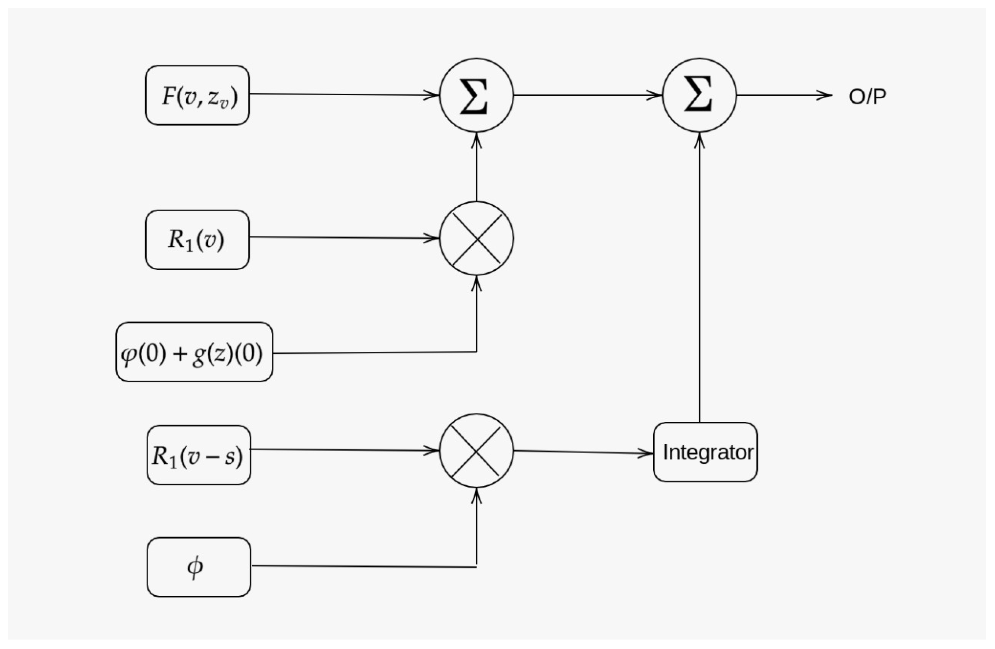
6. Application II—Filter System

Digital filters are easily understood and calculated. The practical challenges of their design and implementation are significant and are the subject of much advanced research. A digital filter is a system that performs mathematical operations on a sampled, discrete time signal to reduce or enhance certain aspects of that signal. A variety of mathematical techniques may be employed to analyze the behavior of a given digital filter. There are two categories of digital filters, such as infinite impulse response (IIR) filters and finite impulse response (FIR) filters. For example, the FIR filter is often used to smooth a random process to suppress noise and bring out a slower-varying signal and the detection of a signal in a noisy background with a matched filter.

In [17,18], the authors discussed the methodology for an upgraded framework of FIR from the software level to the hardware level. Moreover, in [19], the authors discussed the coupling between an asynchronas designs and non-uniform sampling schemes in order to implement a digital filter. In [20,21], the authors discussed the reconstruction of the speech signal, and compared FIR and IIR filter banks and also studied the transfer functions related to one-dimensional and two-dimensional filter systems. Motivated by the above works, we present our filter system shown in Figure 1, which describes the rough pattern of a block diagram. it provides the solutions with respect to a minimum number of inputs with high accuracy and fast execution time.

Figure 1. Filter diagram.

1.

Product modulator (PM)-1 accepts the inputs $R_1\left(v\right)$ and $\left[\phi \right(0)+g(z\left)\right(0\left)\right]$ at time $v=0$, and produces the output $R_1\left(v\right)[\phi \left(0\right)+g\left(z\right)\left(0\right)]$.

2.

PM-2 accepts the inputs $R_1(v-s)$ and $\varphi$, and produces the output $R_1(v-s)\varphi$.

3.

The integrator executes the integral of $R_1(v-s)\varphi$ over the period v.

Finally, the input $F(v,z_v)$, the output from PM-1, and the output from the integrator are moved to the summer network; then we will get output $z\left(v\right)$.

7. Conclusions

This manuscript illustrates that the existence of a mild solution for the neutral partial integrodifferential nonlocal system with finite delay is supported by a Monch–Krasnosel’skii type fixed point theorem, measure of noncompactness, and resolvent operator theory. Finally, we have constructed a rough filter system associated with our existence result.

References

1. Chen, C.; Grimmer, R. Semigroups and integral equations. J. Integral Equ. 1980, 2, 133–154. [Google Scholar]
2. Grimmer, R.C. Resolvent operators for integral equations in a Banach space. Trans. Am. Math. Soc. 1982, 273, 333–349. [Google Scholar] [CrossRef]
3. Balachandran, K.; Shija, G. Existence of Solutions of Nonlinear Abstract Neutral Integrodifferential Equations. Comput. Math. Appl. 2004, 48, 1403–1414. [Google Scholar] [CrossRef] [Green Version]
4. Ezzinbi, K.; Ghnimi, S.; Taoudi, M.A. New Monch-Krasnosel’skii type fixed point theorems applied to solve neutral partial integrodifferential equations without compactness. J. Fixed Point Theory Appl. 2020, 22, 73. [Google Scholar] [CrossRef]
5. Hernandez, E. Existence results for partial neutral functional integrodifferential equations with unbounded delay. J. Math. Anal. Appl. 2004, 292, 194–210. [Google Scholar] [CrossRef]
6. Murugesu, R.; Suguna, S. Existence of solutions for neutral functional integrodifferential equations. Tamkang J. Math. 2010, 41, 117–128. [Google Scholar] [CrossRef]
7. Pazy, A. Semigroups of Linear Operators and Applications to Partial Differential Equations; Springer: New York, NY, USA, 1983. [Google Scholar]
8. Lizama, C.; Pozo, J.C. Existence of mild solutions for a semilinear integrodifferential equation with nonlocal initial conditions. Abstr. Appl. Anal. 2012, 2012, 1–15. [Google Scholar] [CrossRef]
9. Ezzinbi, K.; Ghnimi, S. Existence and Regularity for Some Partial Neutral Functional Integrodifferential Equations with Nondense Domain. Bull. Malays. Math. Sci. Soc. 2019, 43, 1–21. [Google Scholar] [CrossRef]
10. Banas, J.; Goebel, K. Measure of Noncompactness in Banach Spaces; Marcel Dekker: New York, NY, USA, 1980. [Google Scholar]
11. Chlebowicz, A.; Taoudi, M.A. Measures of Weak Noncompactness and Fixed points. In Advances in Nonlinear Analysis via the Concept of Measures of Noncompactness; Springer: Singapore, 2017; pp. 247–296. [Google Scholar]
12. Sun, J.; Zhang, X. The fixed point theorem of convex-power condensing operator and applications to abstract semilinear evolution equations. Acta Math. Sin. 2005, 48, 339–446. [Google Scholar]
13. Henrniquez, H.R.; Poblete, V.; Pozo, J.C. Mild solutions of non-autonomous second order problems with nonlocal initial conditions. J. Math. Anal. Appl. 2014, 412, 1064–1083. [Google Scholar] [CrossRef]
14. Liu, L.; Guo, F.; Wu, C.; Wu, Y. Existence theorems of global solutions for nonlinear Volterra type integral equations in Banach spaces. J. Math. Anal. Appl. 2005, 309, 638–649. [Google Scholar] [CrossRef] [Green Version]
15. Daher, S.D. On a fixed point principle of Sadovskii. Nonlinear Anal. 1978, 2, 643–645. [Google Scholar] [CrossRef]
16. Kamenskii, M.; Obukhovskii, V.; Zekka, P. Condensing Multivated Maps and Semilinear Differential Inclusions in Banach Spaces; De Gryter: Berlin, NY, USA, 2001. [Google Scholar]
17. Chandra, A.; Chattopadhyay, S. Design of hardware efficient FIR filter: A review of the state-of-the-art approaches. Eng. Sci. Technol. Int. J. 2016, 19, 212–226. [Google Scholar] [CrossRef] [Green Version]
18. Zahoor, S.; Naseem, S. Design and implementation of an efficient FIR digital filter. Cogent Eng. 2017, 4, 1323373. [Google Scholar] [CrossRef]
19. Beyrouthy, T.; Fesquet, L. An event-driven FIR filter design and implementation. In Proceedings of the 22nd IEEE International Symposium on Rapid System Prototyping, Karlsruhe, Germany, 24–27 May 2011; pp. 59–65. [Google Scholar]
20. Tabassum, F.; Amin, M.R.; Islam, M.I. Comparison of FIR and IIR Filter Bank in Reconstruction of Speech Signal. Int. J. Comput. Sci. Inf. Secur. 2016, 14, 864–872. [Google Scholar]
21. Stavrou, V.N.; Tsoulos, I.G.; Mastorakis, N.E. Transformations for FIR and IIR Filters Design. Symmetry 2021, 33, 533. [Google Scholar] [CrossRef]