Analytical Solution of Coupled Hirota–Satsuma and KdV Equations

Abstract

In this study, we applied the Laplace residual power series method (LRPSM) to expand the solution of the nonlinear time-fractional coupled Hirota–Satsuma and KdV equations in the form of a rapidly convergent series while considering Caputo fractional derivatives. We demonstrate the applicability and accuracy of the proposed method with some examples. The numerical results and the graphical representations reveal that the proposed method performs extremely well in terms of efficiency and simplicity. Therefore, it can be utilized to solve more problems in the field of non-linear fractional differential equations. To show the validity of the proposed method, we present a numerical application, compute two kinds of errors, and sketch figures of the obtained results.

1. Introduction

Fractional differential equations are a generalized form of ordinary and partial differential equations [1,2,3,4]. Recently, various studies in engineering and sciences have confirmed that the dynamics of numerous systems in nature can be described more precisely via nonlinear fractional-order differential equations, for instance, in biology, physics, engineering, chaos theory, diffusion, electromagnetism, etc. [5,6,7,8,9,10,11]. Therefore, several approaches have been established to acquire approximate and analytic solutions of fractional differential equations, including the variational iteration method [12], the differential transform method [13,14,15], Laplace transforms [16,17], the fractional sub-equation method [18,19], the homotopy perturbation method [20,21], the exponential rational function method [22], the exponential function method [23], the extended trial equation method [24], the ARA residual power series method [25], the double ARA–Sumudu transform [26], and the reproducing kernel method [27], amongst others.

The power series method [28] is one of the most popular and convenient methods used to establish analytic solutions for linear classes of differential equations. Unfortunately, obtaining a closed-form solution for the nonlinear case is very difficult or impossible. Therefore, the residual power series method is introduced to overcome the aforementioned difficulty of the power series method. The residual power series method [29,30] has been employed to gain the analytical solution of various linear and nonlinear models in different engineering and science areas.

This article develops the residual power series method by employing the Laplace transform (LT) [31] in its methodology. This promotion is known as the Laplace residual power series method (LRPSM). In contrast with other power series methods, LRPSM requires less time and simpler computation but has superior accuracy in obtaining the solution. Moreover, the LRPSM needs no differentiation or linearization: it depends only on applying the LT and taking the limit at infinity. Due to these advantages, various researchers have used it to solve nonlinear fractional problems [29,30,32,33,34].

In this study, the LRPSM is introduced to solve the coupled Hirota–Satsuma and KdV (HSC–KdV) equations of the form:

$$\begin{gathered} D_{\tau }^{\alpha }\delta =\frac{1}{2}{\delta }_{\xi \xi \xi }-3\delta {\delta }_{\xi }+3{(\varphi \psi )}_{\xi }, \\ \left(1\right)D_{\tau }^{\alpha }\varphi =-{\varphi }_{\xi \xi \xi }+3\delta {\varphi }_{\xi }, \\ \left(2\right)D_{\tau }^{\alpha }\psi =-{\psi }_{\xi \xi \xi }+3\delta {\psi }_{\xi }, \end{gathered}$$

where $\delta \left(\xi ,\tau \right), \varphi \left(\xi ,\tau \right), \mathrm{and} \psi \left(\xi ,\tau \right)$ are three unknown functions of the independent variables $\xi \mathrm{and} \tau ,$ and $D_{\tau }^{\alpha }$ is the time Caputo fractional operator with $0<\alpha \le 1$.

The HSC–KdV equations are of great significance due to their numerous applications in diverse areas. For instance, the HSC–KdV equations are used to represent the dispersive long waves in shallow water which are employed in many implementations in fluid mechanics, including shallow-water undulations with weakly non-linear retrieve vigor, acoustic undulations on a crystal lattice, long inner undulations in a density-stratified ocean, and ion-acoustic undulations in a plasma [35].

The novelty of this work arises in the chosen model, which is difficult to solve by traditional numerical methods: some authors have solved this system numerically and obtained only the first two or three terms of the approximate solution, but not a general term of the series solution. In contrast, the LRPSM allows us to obtain many terms of the series solution easily, using Mathematica software. LRPS is a powerful technique for solving fractional models, and it presents the solution in a form of a rapidly convergent series with less effort and computation than other numerical methods. It also requires no differentiation or linearization, only computing the limit at infinity.

The description of this article is as follows: we start in Section 2 by presenting some fundamental concepts and preliminary results from the fractional calculus theory. In Section 3, we assemble the algorithm of LRPSM for obtaining the solution of the HSC–KdV. Section 4 presents some HSC–KdV problems to demonstrate the simplicity, capability, and potentiality of LRPSM, and Section 5 concludes the paper.

2. Basic Preliminaries

This section introduces some basic notations, definitions, and theorems related to fractional calculus which are utilized throughout this article.

2.1. Fractional Power Series

Here, we present some definitions of the Caputo fractional derivative and Laplace transform. We also introduce some theorems related to fractional power series representations.

Definition 1.

The Caputo derivative of fractional order$\alpha \in R^{+}$of the function$x\left(\tau \right)$is given by:

$$D^{\alpha }x\left(\tau \right)=\left\{\begin{array}{cc}\frac{1}{\Gamma \left(\mu -\alpha \right)}\underset{0}{\overset{\tau }{{\displaystyle \int }}}\frac{x^{\left(\mu \right)}\left(t\right)}{{\left(\tau -t\right)}^{\alpha +1-\mu }}dt,& \mu -1<\alpha <\mu ,\\ x^{\left(\mu \right)}\left(\tau \right)& \alpha =\mu ,\hspace{1em}\mu \in \mathbb{N}.\end{array}\right.$$

Definition 2

([36]). The time Caputo derivative of fractional order $\alpha \in R^{+}$ of the function $x\left(\xi ,\tau \right)$ is given by:

$$D_{\tau }^{\alpha }x\left(\xi ,\tau \right)=\frac{{\partial }^{\alpha }x\left(\xi ,\tau \right)}{\partial {\tau }^{\alpha }}=\left\{\begin{array}{cc}\frac{1}{\Gamma \left(\mu -\alpha \right)}\underset{0}{\overset{\tau }{{\displaystyle \int }}}{\left(\tau -t\right)}^{\mu -\alpha -1}\frac{{\partial }^{\mu }x\left(\xi ,t\right)}{\partial t^{\mu }}\partial t,& \mu -1<\alpha <\mu ,\\ \frac{{\partial }^{\mu }x\left(\xi ,\tau \right)}{\partial {\tau }^{\mu }}& \alpha =\mu ,\hspace{1em}\mu \in \mathbb{N}.\end{array}\right.$$

Definition 3

([31]). The Laplace transform of a function $x\left(\xi ,\tau \right)$ regarding the variable $\tau$ is defined as:

$$\mathcal{L}\left[x\left(\xi ,\tau \right)\right]=X\left(\xi ,s\right)=\underset{0}{\overset{\infty }{{\displaystyle \int }}}x\left(\xi ,\tau \right)e^{-s\tau }d\tau ,\hspace{1em}\hspace{1em}s>0,$$

and the inverse LT is given by:

$$x\left(\xi ,\tau \right)={\mathcal{L}}^{-1}\left[X\left(\xi ,s\right)\right]=\underset{c-i\infty }{\overset{c+i\infty }{{\displaystyle \int }}}X\left(\xi ,s\right)e^{st}ds,\hspace{1em}\hspace{1em}c=Re\left(s\right)>0.$$

Further, if $\mathcal{L}\left[x_1\left(\xi ,\tau \right)\right]=X_1\left(\xi ,s\right)$ and $\mathcal{L}\left[x_2\left(\xi ,\tau \right)\right]=X_2\left(\xi ,s\right)$ and considering ${\gamma }_1$ and ${\gamma }_2$ are two real constants, we have the following essential properties of Laplace transform, and its inverse [29,30]:

• $\mathcal{L}\left[{\gamma }_1 x_1\left(\xi ,\tau \right)+{\gamma }_2 x_2\left(\xi ,\tau \right)\right]={\gamma }_1{X}_1\left(\xi ,s\right)+{\gamma }_2{X}_2\left(\xi ,s\right).$
• ${\mathcal{L}}^{-1}\left[{\gamma }_1 X_1\left(\xi ,s\right)+{\gamma }_2 X_2\left(\xi ,s\right)\right]={\gamma }_1{x}_1\left(\xi ,\tau \right)+{\gamma }_2{x}_2\left(\xi ,\tau \right).$
• $\mathcal{L}\left[{\tau }^{\vartheta }\right]=\frac{\mathsf{\Gamma }\left(\vartheta +1\right)}{s^{\vartheta +1}},\vartheta >-1.$
• $\mathcal{L}\left[D_{\tau }^{\alpha }x\left(\xi ,\tau \right)\right]=s^{\alpha }X\left(\xi ,s\right)-{{\displaystyle \sum }}_{l=0}^{\mu -1}{s}^{\alpha -l-1}{D}_{\tau }^{l}x\left(\xi ,\tau \right), \mu -1<\alpha <\mu , \mu \in \mathbb{N}.$

Definition 4

([29,30]). A fractional power series of two variables around ${\tau }_0=0$ is expressed as:

$${\displaystyle \sum }_{m=0}^{\infty }{a}_m\left(\xi \right){\tau }^{m\alpha }=a_0\left(\xi \right)+a_1\left(\xi \right){\tau }^{\alpha }+\cdots ,\hspace{1em}0\le \mu -1<\alpha <\mu ,\hspace{1em}\hspace{1em}\tau <0.$$

Theorem 1.

Suppose that a function$x$has a FPS expansion at${\tau }_0=0$of the form:

$$x\left(\xi ,\tau \right)={\displaystyle \sum }_{m=0}^{\infty }{a}_m\left(\xi \right){\tau }^{m\alpha },\hspace{1em}\hspace{1em}0\le \tau <{\rm T},$$

(1)

where$T$is the radius of convergence of the fractional power series. If$D_{\tau }^{\alpha } x\left(\xi ,\tau \right)$is continuous on$I\times \left[0,R\right]$, then the coefficients$a_m\left(\xi \right)$can be written as:

$$a_m\left(\xi \right)=\frac{D_{\tau }^{m\alpha }x\left(\xi ,0\right)}{\Gamma \left(m\alpha +1\right)},\hspace{1em}\hspace{1em}m=0,1,2,\dots ,$$

where$D_{\tau }^{m\alpha }=D_{\tau }^{\alpha }·D_{\tau }^{\alpha }\dots D_{\tau }^{\alpha }$ (m-times). For the proof, refer to [37].

Using Theorem 1, the fractional power series expansion of the $x\left(\xi ,\tau \right)$ around $\tau =0$ is given by:

$$x\left(\xi ,\tau \right)={\displaystyle \sum }_{m=0}^{\infty }\frac{D_{\tau }^{m\alpha }x\left(\xi ,0\right)}{\mathsf{\Gamma }\left(m\alpha +1\right)}{\tau }^{m\alpha },\hspace{1em}0\le \mu -1<\alpha <\mu ,\hspace{1em}\xi \in I,\hspace{1em}0\le \tau <{\rm T}.$$

2.2. Convergence Analysis of LRPSM

This section covers the conditions of convergence for the new fractional power series in the Laplace space. It is worth mentioning here that the Laplace residual power series approach requires the same conditions of convergence as the usual Taylor’s series.

Theorem 2

([30]). If the function $X\left(\xi ,s\right)=\mathcal{L}\left[x\left(\xi ,\tau \right)\right]$ has the fractional power series:

$$X\left(\xi ,s\right)={\displaystyle \sum }_{m=0}^{\infty }\frac{a_m\left(\xi \right)}{s^{m\alpha +1}},\hspace{1em}\hspace{1em}0<\alpha \le 1,s>0.$$

(2)

then $a_m\left(\xi \right)=D_{\tau }^{m\alpha }x\left(\xi ,0\right)$, where $D_{\tau }^{m\alpha }=D_{\tau }^{\alpha }·D_{\tau }^{\alpha }\dots D_{\tau }^{\alpha }$ (m-times). Moreover, the inverse LT of (2) is defined by:

$$x\left(\xi ,\tau \right)={\displaystyle \sum }_{m=0}^{\infty }\frac{D_{\tau }^{m\alpha }x\left(\xi ,0\right)}{\mathsf{\Gamma }\left(m\alpha +1\right)}{\tau }^{m\alpha },\hspace{1em}\hspace{1em}0<\alpha \le 1, \tau \ge 0.$$

Theorem 3

([30]). Suppose that:

$$\left|s\mathcal{L}\left[D_{\tau }^{\left(m+1\right)\alpha } x\left(\xi ,\tau \right)\right]\right|\le H$$

for ${\delta }_1<s\le {\delta }_2$ and $\xi \in I$ , where $H=H\left(\xi \right)$ and $0<\alpha \le 1$. Then, the remainder $R_m\left(\xi ,s\right)$ in (2) fulfills:

$$\left|R_m\left(\xi ,s\right)\right|\le \frac{H}{s^{\left(m+1\right)\alpha +1}},\xi \in I \mathrm{and} {\delta }_1<s\le {\delta }_2.$$

Proof of Theorem 3.

First, we suppose that $\mathcal{L}\left[D_{\tau }^{m\alpha } x\left(\xi ,\tau \right)\right]\left(s\right)$ is defined on $I\times \left({\delta }_1,\left.{\delta }_2\right]\right.$, for $m=0,1,2\dots ,n+1$. As given, we also assume that:

$$\left|s\mathcal{L}\left[D_{\tau }^{\left(m+1\right)\alpha } x\left(\xi ,\tau \right)\right]\right|\le H\left(\xi \right),\xi \in I \mathrm{and} {\delta }_1<s\le {\delta }_2.$$

(3)

The definition of the remainder implies:

$$R_m\left(\xi ,s\right)=X\left(\xi ,s\right)-{\displaystyle \sum }_{k=0}^m\frac{D_{\tau }^{k\alpha }x\left(\xi ,0\right)}{s^{k\alpha +1}},$$

thus, one can obtain:

$$\begin{array}{ll}{s}^{1+\left(m+1\right)\alpha }{R}_m\left(\xi ,s\right)& =s^{1+\left(m+1\right)\alpha }X\left(\xi ,s\right)-{\displaystyle {\displaystyle \sum }_{k=0}^m}{s}^{\left(m+1-k\right)\alpha }{D}_{\tau }^{k\alpha }x\left(\xi ,0\right)\\ & =s\left(s^{\left(m+1\right)\alpha }X\left(\xi ,s\right)-{\displaystyle {\displaystyle \sum }_{k=0}^m}{s}^{\left(m+1-k\right)\alpha -1}{D}_{\tau }^{k\alpha }x\left(\xi ,0\right)\right)\\ & =s\mathcal{L}\left[D_{\tau }^{\left(m+1\right)\alpha } x\left(\xi ,\tau \right)\right].\end{array}$$

(4)

Equations (3) and (4) imply that $\left|s^{1+\left(m+1\right)\alpha }{R}_m\left(\xi ,s\right)\right|\le H\left(\xi \right)$.

Hence $-H\left(x\right)\le s^{1+\left(m+1\right)\alpha }{R}_m\left(\xi ,s\right)\le H\left(\xi \right),\xi \in I, {\delta }_1<s\le {\delta }_2$.

Thus, reformulating the above equation, we can obtain the result. □

Theorem 4

([33]). Assume that $\Vert x_{n+1}\left(\xi ,\tau \right)\Vert \le \epsilon \Vert x_n\left(\xi ,\tau \right)\Vert , \forall n\in N$ for some $\epsilon \in \left(0,1\right),$ and $0<\tau <T<1$; then, the obtained approximate series solution converges to the exact one, where:

$$x_n\left(\xi ,\tau \right)={\displaystyle \sum }_{m=0}^n\frac{D_{\tau }^{m\alpha }x\left(\xi ,0\right)}{\Gamma \left(m\alpha +1\right)}{\tau }^{m\alpha }.$$

Proof of Theorem 4.

Notice that, if $0<\tau <T<1$, then:

$$\begin{gathered} \Vert x\left(\xi ,\tau \right)-x_n\left(\xi ,\tau \right)\Vert \le \Vert {\displaystyle \sum }_{m=n+1}^{\infty }{x}_m\left(\xi ,\tau \right)\Vert \le {\displaystyle \sum }_{m=n+1}^{\infty }\Vert x_m\left(\xi ,\tau \right)\Vert , \forall 0<\tau <T<1. \\ \Vert x\left(\xi ,\tau \right)-x_n\left(\xi ,\tau \right)\Vert \le \Vert g\left(y\right)\Vert \Vert {\displaystyle \sum }_{m=n+1}^{\infty }{\epsilon }^m\Vert =\frac{{\epsilon }^{m+1}}{1-\epsilon }\Vert g\left(y\right)\Vert \underset{n\to \infty }{\to }0. \end{gathered}$$

□

3. LRPSM Methodology

In this section, we apply the LRPSM to solve HSC–KdV equations. The main idea of the LRPSM is to first apply the Laplace transform on the target equation and then define the so-called Laplace residual function. Then, using some facts of the residual power series method and taking the limit at infinity allows us to obtain the coefficients of the series solutions.

Now, we consider the system:

$$\left.\begin{array}{c}{D}_{\tau }^{\alpha }\delta =\frac{1}{2}{\delta }_{\xi \xi \xi }-3\delta {\delta }_{\xi }+3{(\varphi \psi )}_{\xi },\\ D_{\tau }^{\alpha }\varphi =-{\varphi }_{\xi \xi \xi }+3\delta {\varphi }_{\xi },\\ D_{\tau }^{\alpha }\psi =-{\psi }_{\xi \xi \xi }+3\delta {\psi }_{\xi },\end{array}\right\}$$

(5)

subject to the initial conditions (ICs):

$$\delta \left(\xi ,0\right)=a\left(\xi \right),\hspace{1em}\varphi \left(\xi ,0\right)=b\left(\xi \right),\hspace{1em}\psi \left(\xi ,0\right)=c\left(\xi \right).$$

(6)

We illustrate the steps of the LRPSM on system (5) and (6) as follows.

Step 1. Apply the Laplace transform with respect to $\tau$ to each equation in (5) to obtain

$$\begin{gathered} \begin{array}{c}\hspace{1em}\hspace{1em}{s}^{\alpha }\mathcal{G}\left(\xi ,s\right)-s^{\alpha -1}\delta \left(\xi ,0\right)\hfill \\ \hspace{1em}\hspace{1em}\hspace{1em}\hspace{1em}\hspace{1em}\hspace{1em}\hspace{1em}\hspace{1em}=\frac{1}{2} \frac{{\partial }^3}{\partial {\xi }^3}\mathcal{G}\left(\xi ,s\right)-3\mathcal{L}\left[{\mathcal{L}}^{-1}\left[\mathcal{G}\left(\xi ,s\right)\right]\frac{\partial }{\partial \xi }{\mathcal{L}}^{-1}\left[\mathcal{G}\left(\xi ,s\right)\right]\right]\hfill \\ \hspace{1em}\hspace{1em}+3\frac{\partial }{\partial \xi }\left[{\mathcal{L}}^{-1}\left[\mathsf{\Phi }\left(\xi ,s\right)\right] {\mathcal{L}}^{-1}\left[\mathsf{\Psi }\left(\xi ,s\right)\right]\right],\end{array} \\ {s}^{\alpha }\mathsf{\Phi }\left(\xi ,s\right)-s^{\alpha -1}\varphi \left(\xi ,0\right)=-\frac{{\partial }^3}{\partial {\xi }^3}\mathsf{\Phi }\left(\xi ,s\right)+3\mathcal{L}\left[{\mathcal{L}}^{-1}\left[\mathcal{G}\left(\xi ,s\right)\right]·\frac{\partial }{\partial \xi }{\mathcal{L}}^{-1}\left[\mathsf{\Phi }\left(\xi ,s\right)\right]\right], \\ {s}^{\alpha }\mathsf{\Psi }\left(\xi ,s\right)-s^{\alpha -1}\psi \left(\xi ,0\right)=-\frac{{\partial }^3}{\partial {\xi }^3}\mathsf{\Psi }\left(\xi ,s\right)+3\mathcal{L}\left[{\mathcal{L}}^{-1}\left[\mathcal{G}\left(\xi ,s\right)\right]·\frac{\partial }{\partial \xi }{\mathcal{L}}^{-1}\left[\mathsf{\Psi }\left(\xi ,s\right)\right]\right], \end{gathered}$$

(7)

where $\mathcal{G}\left(\xi ,s\right)=\mathcal{L}\left[\delta \left(\xi ,\tau \right)\right],\mathsf{\Phi }\left(\xi ,s\right)=\mathcal{L}\left[\varphi \left(\xi ,\tau \right)\right],$ and $\mathsf{\Psi }\left(\xi ,s\right)=\mathcal{L}\left[\psi \left(\xi ,\tau \right)\right]$.

Simplifying each Equation in (7) and employing the ICs yields:

$$\begin{array}{c}\mathcal{G}\left(\xi ,s\right)=\frac{a\left(\xi \right)}{s}+\frac{1}{2s^{\alpha }} \frac{{\partial }^3}{\partial {\xi }^3}\mathcal{G}\left(\xi ,s\right)-\frac{3}{s^{\alpha }}\mathcal{L}\left[{\mathcal{L}}^{-1}\left[\mathcal{G}\left(\xi ,s\right)\right]·\frac{\partial }{\partial \xi }{\mathcal{L}}^{-1}\left[\mathcal{G}\left(\xi ,s\right)\right]\right]\\ +\frac{3}{s^{\alpha }}\frac{\partial }{\partial \xi }\left[{\mathcal{L}}^{-1}\left[\mathsf{\Phi }\left(\xi ,s\right)\right]·{\mathcal{L}}^{-1}\left[\mathsf{\Psi }\left(\xi ,s\right)\right]\right],\\ \mathsf{\Phi }\left(\xi ,s\right)=\frac{b\left(\xi \right)}{s}-\frac{1}{s^{\alpha }}\frac{{\partial }^3}{\partial {\xi }^3}\mathsf{\Phi }\left(\xi ,s\right)+\frac{3}{s^{\alpha }}\mathcal{L}\left[{\mathcal{L}}^{-1}\left[\mathcal{G}\left(\xi ,s\right)\right]·\frac{\partial }{\partial \xi }{\mathcal{L}}^{-1}\left[\mathsf{\Phi }\left(\xi ,s\right)\right]\right],\\ \mathsf{\Psi }\left(\xi ,s\right)=\frac{c\left(\xi \right)}{s}-\frac{1}{s^{\alpha }}\frac{{\partial }^3}{\partial {\xi }^3}\mathsf{\Psi }\left(\xi ,s\right)+\frac{3}{s^{\alpha }}\mathcal{L}\left[{\mathcal{L}}^{-1}\left[\mathcal{G}\left(\xi ,s\right)\right]·\frac{\partial }{\partial \xi }{\mathcal{L}}^{-1}\left[\mathsf{\Psi }\left(\xi ,s\right)\right]\right].\end{array}$$

(8)

Step 2. Define the series solution of (8), as follows:

$$\begin{gathered} \mathcal{G}\left(\xi ,s\right)={\displaystyle \sum }_{n=0}^{\infty }\frac{{\delta }_n\left(\xi \right)}{s^{n\alpha +1}}, \\ \mathsf{\Phi }\left(\xi ,s\right)={\displaystyle \sum }_{n=0}^{\infty }\frac{{\varphi }_n\left(\xi \right)}{s^{n\alpha +1}}, \end{gathered}$$

and:

$$\mathsf{\Psi }\left(\xi ,s\right)={\displaystyle \sum }_{n=0}^{\infty }\frac{{\psi }_n\left(\xi \right)}{s^{n\alpha +1}}.$$

Using the fact that $\mathcal{L}\left[s \mathcal{G}\left(\xi ,s\right)\right]=\delta \left(\xi ,0\right),$ one can identify the k^th truncated solution of (8) as:

$$\begin{array}{c}{\mathcal{G}}_k\left(\xi ,s\right)=\frac{a\left(\xi \right)}{s}+{\displaystyle {\displaystyle \sum }_{n=1}^k}\frac{{\delta }_n\left(\xi \right)}{s^{n\alpha +1}}, \\ {\mathsf{\Phi }}_k\left(\xi ,s\right)=\frac{b\left(\xi \right)}{s}+{\displaystyle {\displaystyle \sum }_{n=1}^k}\frac{{\varphi }_n\left(\xi \right)}{s^{n\alpha +1}},\\ {\mathsf{\Psi }}_k\left(\xi ,s\right)=\frac{c\left(\xi \right)}{s}+{\displaystyle {\displaystyle \sum }_{n=1}^k}\frac{{\psi }_n\left(\xi \right)}{s^{n\alpha +1}}.\end{array}$$

(9)

Step 3. Define the k^th Laplace residual functions of (8) as:

$$\begin{array}{c}\mathcal{L}{\mathrm{Res}}_k\mathcal{G}\left(\xi ,s\right)={\mathcal{G}}_k\left(\xi ,s\right)-\frac{a\left(\xi \right)}{s}-\frac{1}{2s^{\alpha }} \frac{{\partial }^3}{\partial {\xi }^3}\mathcal{G}\left(\xi ,s\right)\\ \hspace{1em}\hspace{1em}\hspace{1em}\hspace{1em}\hspace{1em}\hspace{1em}\hspace{1em}\hspace{1em}\hspace{1em}+\frac{3}{s^{\alpha }}\mathcal{L}\left[{\mathcal{L}}^{-1}\left[{\mathcal{G}}_k\left(\xi ,s\right)\right]·\frac{\partial }{\partial \xi }{\mathcal{L}}^{-1}\left[{\mathcal{G}}_k\left(\xi ,s\right)\right]\right]\\ \hspace{1em}\hspace{1em}\hspace{1em}\hspace{1em}\hspace{1em}\hspace{1em}\hspace{1em}\hspace{1em}\hspace{1em}-\frac{3}{s^{\alpha }}\frac{\partial }{\partial \xi }\left[{\mathcal{L}}^{-1}\left[{\mathsf{\Phi }}_k\left(\xi ,s\right)\right]·{\mathcal{L}}^{-1}\left[{\mathsf{\Psi }}_k\left(\xi ,s\right)\right]\right],\\ \mathcal{L}{\mathrm{Res}}_k\mathsf{\Phi }\left(\xi ,s\right)={\mathsf{\Phi }}_k\left(\xi ,s\right)-\frac{b\left(\xi \right)}{s}+\frac{1}{s^{\alpha }} \frac{{\partial }^3}{\partial {\xi }^3}{\mathsf{\Phi }}_k\left(\xi ,s\right)\\ \hspace{1em}\hspace{1em}\hspace{1em}\hspace{1em}\hspace{1em}\hspace{1em}\hspace{1em}\hspace{1em}\hspace{1em}-\frac{3}{s^{\alpha }}\mathcal{L}\left[{\mathcal{L}}^{-1}\left[{\mathcal{G}}_k\left(\xi ,s\right)\right]·\frac{\partial }{\partial \xi }{\mathcal{L}}^{-1}\left[{\mathsf{\Phi }}_k\left(\xi ,s\right)\right]\right],\\ \mathcal{L}{\mathrm{Res}}_k\mathsf{\Psi }\left(\xi ,s\right)={\mathsf{\Psi }}_k\left(\xi ,s\right)-\frac{c\left(\xi \right)}{s}+\frac{3}{s^{\alpha }}\frac{{\partial }^3}{\partial {\xi }^3}{\mathsf{\Psi }}_k\left(\xi ,s\right)\\ \hspace{1em}\hspace{1em}\hspace{1em}\hspace{1em}\hspace{1em}\hspace{1em}\hspace{1em}\hspace{1em}\hspace{1em}-\frac{3}{s^{\alpha }}\mathcal{L}\left[{\mathcal{L}}^{-1}\left[{\mathcal{G}}_k\left(\xi ,s\right)\right]·\frac{\partial }{\partial \xi }{\mathcal{L}}^{-1}\left[{\mathsf{\Psi }}_k\left(\xi ,s\right)\right]\right].\end{array}$$

(10)

Step 4. To find the first coefficients of the truncated series solution (9), we define the first truncated solution and substitute it in the first truncated Laplace residual functions as:

$$\begin{array}{c}\mathcal{L}{\mathrm{Res}}_1\mathcal{G}\left(\xi ,s\right)=\frac{{\delta }_1\left(\xi \right)}{s^{\alpha +1}}-\frac{1}{2s^{\alpha }} \frac{{\partial }^3}{\partial {\xi }^3}\left[\frac{a\left(\xi \right)}{s}+\frac{{\delta }_1\left(\xi \right)}{s^{\alpha +1}}\right]\hspace{1em}\hspace{1em}\hspace{1em}\hspace{1em}\hspace{1em}\hspace{1em}\hspace{1em}\hspace{1em}\hspace{1em}\hfill \\ \hfill +\frac{3}{s^{\alpha }}\mathcal{L}\left[{\mathcal{L}}^{-1}\left[\frac{a\left(\xi \right)}{s}+\frac{{\delta }_1\left(\xi \right)}{s^{\alpha +1}}\right] \frac{\partial }{\partial \xi }{\mathcal{L}}^{-1}\left[\frac{a\left(\xi \right)}{s}+\frac{{\delta }_1\left(\xi \right)}{s^{\alpha +1}}\right]\right]\hspace{1em}\\ \hfill -\frac{3}{s^{\alpha }}\frac{\partial }{\partial \xi }\left[{\mathcal{L}}^{-1}\left[\frac{b\left(\xi \right)}{s}+\frac{{\varphi }_1\left(\xi \right)}{s^{\alpha +1}}\right] {\mathcal{L}}^{-1}\left[\frac{c\left(\xi \right)}{s}+\frac{{\psi }_1\left(\xi \right)}{s^{\alpha +1}}\right]\right]=0,\\ \mathcal{L}{\mathrm{Res}}_1\mathsf{\Phi }\left(\xi ,s\right)=\frac{{\varphi }_1\left(\xi \right)}{s^{\alpha +1}}+\frac{1}{s^{\alpha }}\frac{{\partial }^3}{\partial {\xi }^3}\left[\frac{b\left(\xi \right)}{s}+\frac{{\varphi }_1\left(\xi \right)}{s^{\alpha +1}}\right]\hfill \\ \hfill -\frac{3}{s^{\alpha }}\mathcal{L}\left[{\mathcal{L}}^{-1}\left[\frac{a\left(\xi \right)}{s}+\frac{{\delta }_1\left(\xi \right)}{s^{\alpha +1}}\right] \frac{\partial }{\partial \xi }{\mathcal{L}}^{-1}\left[\frac{b\left(\xi \right)}{s}+\frac{{\varphi }_1\left(\xi \right)}{s^{\alpha +1}}\right]\right],\\ \mathcal{L}{\mathrm{Res}}_1\mathsf{\Psi }\left(\xi ,s\right)=\frac{{\psi }_1\left(\xi \right)}{s^{\alpha +1}}+\frac{1}{s^{\alpha }}\frac{{\partial }^3}{\partial {\xi }^3}\left[\frac{c\left(\xi \right)}{s}+\frac{{\psi }_1\left(\xi \right)}{s^{\alpha +1}}\right]\hfill \\ \hfill -\frac{3}{s^{\alpha }}\mathcal{L}\left[{\mathcal{L}}^{-1}\left[\frac{a\left(\xi \right)}{s}+\frac{{\delta }_1\left(\xi \right)}{s^{\alpha +1}}\right] \frac{\partial }{\partial \xi }{\mathcal{L}}^{-1}\left[\frac{c\left(\xi \right)}{s}+\frac{{\psi }_1\left(\xi \right)}{s^{\alpha +1}}\right]\right].\end{array}$$

(11)

Step 5. Recall the succeeding facts that appear in the LRPSM [29], as follows:

• $\mathcal{L}\mathrm{Res}\left(\xi ,s\right)=0$ and $\underset{k\to \infty }{\lim }\mathcal{L}{\mathrm{Res}}_k\left(\xi ,s\right)=\mathcal{L}\mathrm{Res}\left(\xi ,s\right)$, for all $s>0$.
• $\underset{s\to \infty }{\lim }s\mathcal{L}\mathrm{Res}\left(\xi ,s\right)=0$ implies that $\underset{s\to \infty }{\lim }s\mathcal{L}{\mathrm{Res}}_k\left(\xi ,s\right)=0.$
• $\underset{s\to \infty }{\lim }{s}^{k\alpha +1}\mathcal{L}\mathrm{Res}\left(\xi ,s\right)=\underset{s\to \infty }{\lim }{s}^{k\alpha +1}\mathcal{L}{\mathrm{Res}}_k\left(\xi ,s\right)=0, 0<\alpha \le 1, k=1,2,\cdots .$

Now, by multiplying each equation in (11) by $s^{\alpha +1}$ and taking the limit as $s\to \infty ,$ we obtain the first unknowns of the series solutions (9) as:

$$\begin{gathered} {\delta }_1\left(\xi \right)=\frac{1}{2}\left({\delta }^{‴}\left(\xi \right)-6\delta \left(\xi \right){\delta }^{\prime }\left(\xi \right)+6\psi \left(\xi \right){\varphi }^{\prime }\left(\xi \right)+6\varphi \left(\xi \right){\psi }^{\prime }\left(\xi \right)\right) \\ {\varphi }_1\left(\xi \right)=3\delta \left(\xi \right){\varphi }^{\prime }\left(\xi \right)-{\varphi }^{‴}\left(\xi \right) \\ {\psi }_1\left(\xi \right)=3\delta \left(\xi \right){\psi }^{\prime }\left(\xi \right)-{\psi }^{‴}\left(\xi \right) \end{gathered}$$

Repeating the previous steps, one can obtain the second series coefficients recursively, as follows:

$$\begin{array}{l}\hspace{1em}{\delta }_2\left(\xi \right)=\frac{1}{4}{\delta }^{\left(6\right)}\left(\xi \right)+9\delta {\left(\xi \right)}^2\left({\delta }^{″}\left(\xi \right)+3{\psi }^{\prime }\left(\xi \right){\varphi }^{″}\left(\xi \right)+3{\psi }^{″}\left(\xi \right){\varphi }^{\prime }\left(\xi \right)\right)-\frac{9}{2}{\delta }^{″}{\left(\xi \right)}^2\\ \hspace{1em}\hspace{1em}\hspace{1em}\hspace{1em}\hspace{1em}\hspace{1em}\hspace{1em}-9{\varphi }^{‴}\left(\xi \right){\delta }^{\prime }\left(\xi \right){\psi }^{\prime }\left(\xi \right)-9{\psi }^{‴}\left(\xi \right){\delta }^{\prime }\left(\xi \right){\varphi }^{\prime }\left(\xi \right)\\ \hspace{1em}\hspace{1em}\hspace{1em}\hspace{1em}\hspace{1em}\hspace{1em}\hspace{1em}+\varphi \left(\xi \right)\left(\frac{3}{2}{\psi }^{\left(4\right)}\left(\xi \right)-9{\delta }^{\prime }\left(\xi \right){\psi }^{\prime }\left(\xi \right)\right)\\ \hspace{1em}\hspace{1em}\hspace{1em}\hspace{1em}\hspace{1em}\hspace{1em}\hspace{1em}+3\delta \left(\xi \right)(-{\delta }^{\left(4\right)}\left(\xi \right)+18{\delta }^{\prime }\left(\xi \right){\psi }^{\prime }\left(\xi \right){\varphi }^{\prime }\left(\xi \right)+6{\delta }^{\prime }{\left(\xi \right)}^2-3{\varphi }^{\left(4\right)}\left(\xi \right){\psi }^{\prime }\left(\xi \right)\\ \hspace{1em}\hspace{1em}\hspace{1em}\hspace{1em}\hspace{1em}\hspace{1em}\hspace{1em}-3{\varphi }^{‴}\left(\xi \right){\psi }^{″}\left(\xi \right)-3{\psi }^{‴}\left(\xi \right){\varphi }^{″}\left(\xi \right)-3\left({\psi }^{\left(4\right)}\left(\xi \right)+{\psi }^{\prime }\left(\xi \right)\right){\varphi }^{\prime }\left(\xi \right)\\ \hspace{1em}\hspace{1em}\hspace{1em}\hspace{1em}\hspace{1em}\hspace{1em}\hspace{1em}-3\varphi \left(\xi \right){\psi }^{″}\left(\xi \right))-\frac{15}{2}{\delta }^{‴}\left(\xi \right){\delta }^{\prime }\left(\xi \right)+3{\psi }^{‴}\left(\xi \right){\varphi }^{\left(4\right)}\left(\xi \right)-\frac{3}{2}\psi \left(\xi \right){\varphi }^{\left(4\right)}\left(\xi \right)\\ \hspace{1em}\hspace{1em}\hspace{1em}\hspace{1em}\hspace{1em}\hspace{1em}\hspace{1em}+3{\psi }^{\left(4\right)}\left(\xi \right){\varphi }^{‴}\left(\xi \right)+3{\varphi }^{‴}\left(\xi \right){\psi }^{\prime }\left(\xi \right)+9{\psi }^{″}\left(\xi \right){\varphi }^{″}\left(\xi \right)+6{\psi }^{‴}\left(\xi \right){\varphi }^{\prime }\left(\xi \right),\\ {\varphi }_2\left(\xi \right)=-\frac{3}{2}{\delta }^{‴}\left(\xi \right){\varphi }^{\prime }\left(\xi \right)-9{\delta }^{″}\left(\xi \right){\varphi }^{″}\left(\xi \right)-9{\varphi }^{‴}\left(\xi \right){\delta }^{\prime }\left(\xi \right)-6\delta \left(\xi \right){\varphi }^{\left(4\right)}\left(\xi \right)+9\delta {\left(\xi \right)}^2{\varphi }^{″}\left(\xi \right)\\ \hspace{1em}\hspace{1em}\hspace{1em}\hspace{1em}\hspace{1em}\hspace{1em}\hspace{1em}+{\varphi }^{\left(6\right)}\left(\xi \right)+9\varphi \left(\xi \right){\psi }^{\prime }\left(\xi \right){\varphi }^{\prime }\left(\xi \right)+9\psi \left(\xi \right){\varphi }^{\prime }{\left(\xi \right)}^2,\\ {\psi }_2\left(\xi \right)=-\frac{3}{2}{\delta }^{‴}\left(\xi \right){\psi }^{\prime }\left(\xi \right)-9{\delta }^{″}\left(\xi \right){\psi }^{″}\left(\xi \right)-9{\psi }^{‴}\left(\xi \right){\delta }^{\prime }\left(\xi \right)-6\delta \left(\xi \right){\psi }^{\left(4\right)}\left(\xi \right)+9\delta {\left(\xi \right)}^2{\psi }^{″}\left(\xi \right)\\ \hspace{1em}\hspace{1em}\hspace{1em}\hspace{1em}\hspace{1em}\hspace{1em}\hspace{1em}+{\psi }^{\left(6\right)}\left(\xi \right)+9\psi \left(\xi \right){\psi }^{\prime }\left(\xi \right){\varphi }^{\prime }\left(\xi \right)+9\varphi \left(\xi \right){\psi }^{\prime }{\left(\xi \right)}^2.\end{array}$$

Continuing in the same manner, we can conclude the following general k^th terms of the series coefficients as:

$$\begin{array}{r}{\delta }_k\left(\xi \right)=\frac{1}{2}{\delta }_{k-1}^{‴}\left(\xi \right)-3{\displaystyle {\displaystyle \sum }_{i=0}^{k-1}}\frac{{\delta }_i\left(\xi \right){\delta }_{k-i-1}^{\prime }\left(\xi \right)\mathsf{\Gamma }\left(\left(k-1\right)\alpha +1\right)}{\mathsf{\Gamma }\left(i \alpha +1\right)\mathsf{\Gamma }\left(\left(k-i-1\right)\alpha +1\right)}\\ +3{\left({\displaystyle {\displaystyle \sum }_{i=0}^{k-1}}\frac{{\varphi }_i\left(\xi \right){\psi }_{k-i}\left(\xi \right)\mathsf{\Gamma }\left(\left(k-1\right)\alpha +1\right)}{\mathsf{\Gamma }\left(i \alpha +1\right)\mathsf{\Gamma }\left(\left(k-i-1\right)\alpha +1\right)}\right)}^{\prime },\\ {\varphi }_k\left(\xi \right)=-{\varphi }_{k-1}^{‴}\left(\xi \right)+3{\displaystyle {\displaystyle \sum }_{i=0}^{k-1}}\frac{{\delta }_i\left(\xi \right){\varphi }_{k-i-1}^{\prime }\left(\xi \right)\mathsf{\Gamma }\left(\left(k-1\right)\alpha +1\right)}{\mathsf{\Gamma }\left(i \alpha +1\right)\mathsf{\Gamma }\left(\left(k-i-1\right)\alpha +1\right)},\\ {\psi }_k\left(\xi \right)=-{\psi }_{k-1}^{‴}\left(\xi \right)+3{\displaystyle {\displaystyle \sum }_{i=0}^{k-1}}\frac{{\delta }_i\left(\xi \right){\psi }_{k-i-1}^{\prime }\left(\xi \right)\mathsf{\Gamma }\left(\left(k-1\right)\alpha +1\right)}{\mathsf{\Gamma }\left(i \alpha +1\right)\mathsf{\Gamma }\left(\left(k-i-1\right)\alpha +1\right)}.\end{array}$$

where $k=1,2, \dots$.

Thus, the $k$^th series solution of (10) can be written as:

$$\begin{array}{cc}{\mathcal{G}}_k\left(\xi ,s\right)=\frac{a\left(\xi \right)}{s}+{\displaystyle {\displaystyle \sum }_{m=1}^k}\frac{{\mathsf{\delta }}_m\left(\xi \right)}{s^{m\alpha +1}},& k=1,2,\dots \\ {\mathsf{\Phi }}_k\left(\xi ,s\right)=\frac{b\left(\xi \right)}{s}+{\displaystyle {\displaystyle \sum }_{m=1}^k}\frac{{\varphi }_m\left(\xi \right)}{s^{m\alpha +1}},& k=1,2,\dots \\ {\mathsf{\Psi }}_k\left(\xi ,s\right)=\frac{c\left(\xi \right)}{s}+{\displaystyle {\displaystyle \sum }_{m=1}^k}\frac{{\psi }_m\left(\xi \right)}{s^{m\alpha +1}}.& k=1,2,\dots \end{array}$$

Therefore, the solution of (5) and (6) in the original space can be expressed as

$$\begin{array}{c}\delta \left(\xi ,\mathsf{\tau }\right)={\delta }_0+\frac{{\delta }_1\left(\xi \right){\tau }^{\alpha }}{\mathsf{\Gamma }\left(\alpha +1\right)}+\frac{{\delta }_2\left(\xi \right){\tau }^{2\alpha }}{\mathsf{\Gamma }\left(2\alpha +1\right)}+\cdots ,\\ \varphi \left(\xi ,\tau \right)={\varphi }_0+\frac{{\varphi }_1\left(\xi \right){\tau }^{\alpha }}{\mathsf{\Gamma }\left(\alpha +1\right)}+\frac{{\varphi }_2\left(\xi \right){\tau }^{2\alpha }}{\mathsf{\Gamma }\left(2\alpha +1\right)}+\cdots ,\\ \psi \left(\xi ,\tau \right)={\psi }_0+\frac{{\psi }_1\left(\xi \right){\tau }^{\alpha }}{\mathsf{\Gamma }\left(\alpha +1\right)}+\frac{{\psi }_2\left(\xi \right){\tau }^{2\alpha }}{\mathsf{\Gamma }\left(2\alpha +1\right)}+\cdots .\end{array}$$

4. Numerical Application

Consider the time-fractional HSC–KdV equations:

$$\begin{array}{c}{D}_{\tau }^{\alpha }\delta \left(\xi ,\tau \right)=\frac{1}{2}{\delta }_{\xi \xi \xi }\left(\xi ,\tau \right)-3\delta \left(\xi ,\tau \right){\delta }_{\xi }\left(\xi ,\tau \right)+3{(\varphi \left(\xi ,\tau \right)\psi \left(\xi ,\tau \right))}_{\xi },\\ D_{\tau }^{\alpha }\varphi \left(\xi ,\tau \right)=-{\varphi }_{\xi \xi \xi }\left(\xi ,\tau \right)+3\delta \left(\xi ,\tau \right){\varphi }_{\xi }\left(\xi ,\tau \right),\\ D_{\tau }^{\alpha }\psi \left(\xi ,\tau \right)=-{\psi }_{\xi \xi \xi }\left(\xi ,\tau \right)+3\delta \left(\xi ,\tau \right){\psi }_{\xi }\left(\xi ,\tau \right),\end{array}$$

(12)

subject to the ICs:

$$\begin{array}{c}\delta \left(\xi ,0\right)=0.4933+0.02{ \tanh }^2\left(0.1 \xi \right),\\ \varphi \left(\xi ,0\right)=-0.0134+0.0134 \tanh \left(0.1 \xi \right),\\ \psi \left(\xi ,0\right)=1.5+1.5 \tanh \left(0.1 \xi \right).\end{array}$$

(13)

To obtain the solution by the LRPSM in the series form about $t=0$, we first apply the LT on both sides of Equation (12) to obtain:

$$\begin{array}{c}\mathcal{L}\left[D_{\tau }^{\alpha }\delta \left(\xi ,\tau \right)\right]=\frac{1}{2}\mathcal{L}\left[{\delta }_{\xi \xi \xi }\left(\xi ,\tau \right)\right]-3\mathcal{L}\left[\delta \left(\xi ,\tau \right){\delta }_{\xi }\left(\xi ,\tau \right)\right]+3\mathcal{L}\left[{(\varphi \left(\xi ,\tau \right)\psi \left(\xi ,\tau \right))}_{\xi }\right],\\ \mathcal{L}\left[D_{\tau }^{\alpha }\varphi \left(\xi ,\tau \right)\right]=-\mathcal{L}\left[{\varphi }_{\xi \xi \xi }\left(\xi ,\tau \right)\right]+3\mathcal{L}\left[\delta \left(\xi ,\tau \right){\varphi }_{\xi }\left(\xi ,\tau \right)\right],\\ \mathcal{L}\left[D_t^{\alpha }f\left(x,t\right)\right]=-\mathcal{L}\left[{\psi }_{\xi \xi \xi }\left(\xi ,\tau \right)\right]+3\mathcal{L}\left[3\delta \left(\xi ,\tau \right){\psi }_{\xi }\left(\xi ,\tau \right)\right].\end{array}$$

Using the ICs (11), we have:

$$\begin{array}{r}\mathcal{G}\left(\xi ,s\right)=\frac{0.4933+0.02{ \tanh }^2\left(0.1 \xi \right)}{s}+\frac{1}{2s^{\alpha }} \frac{{\partial }^3}{\partial {\xi }^3}\mathcal{G}\left(\xi ,s\right)\hfill \\ -\frac{3}{s^{\alpha }}\mathcal{L}\left[{\mathcal{L}}^{-1}\left[\mathcal{G}\left(\xi ,s\right)\right]·\frac{\partial }{\partial \xi }{\mathcal{L}}^{-1}\left[\mathcal{G}\left(\xi ,s\right)\right]\right]\\ +\frac{3}{s^{\alpha }}\frac{\partial }{\partial \xi }\left[{\mathcal{L}}^{-1}\left[\mathsf{\Phi }\left(\xi ,s\right)\right]·{\mathcal{L}}^{-1}\left[\mathsf{\Psi }\left(\xi ,s\right)\right]\right],\\ \mathsf{\Phi }\left(\xi ,s\right)=\frac{-0.0134+0.0134 \tanh \left(0.1\xi \right)}{s}-\frac{1}{s^{\alpha }}\frac{{\partial }^3}{\partial {\xi }^3}\mathsf{\Phi }\left(\xi ,s\right)\hfill \\ +\frac{3}{s^{\alpha }}\mathcal{L}\left[{\mathcal{L}}^{-1}\left[\mathcal{G}\left(\xi ,s\right)\right]·\frac{\partial }{\partial \xi }{\mathcal{L}}^{-1}\left[\mathsf{\Phi }\left(\xi ,s\right)\right]\right],\\ \mathsf{\Psi }\left(\xi ,s\right)=\frac{1.5+1.5 \tanh \left(0.1 \xi \right)}{s}-\frac{1}{s^{\alpha }}\frac{{\partial }^3}{\partial {\xi }^3}\mathsf{\Psi }\left(\xi ,s\right)\hfill \\ +\frac{3}{s^{\alpha }}\mathcal{L}\left[{\mathcal{L}}^{-1}\left[\mathcal{G}\left(\xi ,s\right)\right]·\frac{\partial }{\partial \xi }{\mathcal{L}}^{-1}\left[\mathsf{\Psi }\left(\xi ,s\right)\right]\right].\end{array}$$

(14)

Define the $k$th-truncated series of Equation (14) as:

$$\begin{array}{c}{\mathcal{G}}_k\left(\xi ,s\right)=\frac{0.4933+0.02{ \tanh }^2\left(0.1 \xi \right)}{s}+{\displaystyle {\displaystyle \sum }_{m=1}^k}\frac{{\mathsf{\delta }}_m\left(x\right)}{s^{m\alpha +1}},\hspace{1em}k=1,2,\cdots \\ {\mathsf{\Phi }}_k\left(\xi ,s\right)=\frac{-0.0134+0.0134 \tanh \left(0.1\xi \right)}{s}+{\displaystyle {\displaystyle \sum }_{m=1}^k}\frac{{\varphi }_m\left(x\right)}{s^{m\alpha +1}},\hspace{1em}k=1,2,\cdots \\ {\mathsf{\Psi }}_k\left(\xi ,s\right)=\frac{1.5+1.5 \tanh \left(0.1 \xi \right)}{s}+{\displaystyle {\displaystyle \sum }_{m=1}^k}\frac{{\psi }_m\left(x\right)}{s^{m\alpha +1}},\hspace{1em}k=1,2,\cdots .\end{array}$$

(15)

The $k$^th Laplace residual function of Equation (14) is defined as:

$$\begin{array}{c}\mathcal{L}{\mathrm{Res}}_k{\mathcal{G}}_k\left(\xi ,s\right)={\mathcal{G}}_k\left(\xi ,s\right)-\frac{0.4933 + 0.02{ \tanh }^2\left(0.1 \xi \right)}{s}-\frac{1}{2s^{\alpha }} \frac{{\partial }^3}{\partial {\xi }^3}\mathcal{G}\left(\xi ,s\right)\\ +\frac{3}{s^{\alpha }}\mathcal{L}\left[{\mathcal{L}}^{-1}\left[\mathcal{G}\left(\xi ,s\right)\right]·\frac{\partial }{\partial \xi }{\mathcal{L}}^{-1}\left[\mathcal{G}\left(\xi ,s\right)\right]\right]\\ -\frac{3}{s^{\alpha }}\frac{\partial }{\partial \xi }\left[{\mathcal{L}}^{-1}\left[\mathsf{\Phi }\left(\xi ,s\right)\right]·{\mathcal{L}}^{-1}\left[\mathsf{\Psi }\left(\xi ,s\right)\right]\right],\\ \mathcal{L}{\mathrm{Res}}_k{\mathsf{\Phi }}_k\left(\xi ,s\right)={\mathsf{\Phi }}_k\left(\xi ,s\right)+\frac{0.0134 + 0.0134 \tanh \left(0.1\xi \right)}{s}+\frac{1}{s^{\alpha }}\frac{{\partial }^3}{\partial {\xi }^3}\mathsf{\Phi }\left(\xi ,s\right)\\ -\frac{3}{s^{\alpha }}\mathcal{L}\left[{\mathcal{L}}^{-1}\left[\mathcal{G}\left(\xi ,s\right)\right]·\frac{\partial }{\partial \xi }{\mathcal{L}}^{-1}\left[\mathsf{\Phi }\left(\xi ,s\right)\right]\right],\\ \mathcal{L}{\mathrm{Res}}_k{\mathsf{\Psi }}_k\left(\xi ,s\right)={\mathsf{\Psi }}_k\left(\xi ,s\right)-\frac{1.5 + 1.5 \tanh \left(0.1 \xi \right)}{s}+\frac{1}{s^{\alpha }}\frac{{\partial }^3}{\partial {\xi }^3}\mathsf{\Psi }\left(\xi ,s\right)\\ -\frac{3}{s^{\alpha }}\mathcal{L}\left[{\mathcal{L}}^{-1}\left[\mathcal{G}\left(\xi ,s\right)\right]·\frac{\partial }{\partial \xi }{\mathcal{L}}^{-1}\left[\mathsf{\Psi }\left(\xi ,s\right)\right]\right].\end{array}$$

(16)

Hence, to obtain the values of the coefficients functions ${\mathsf{\delta }}_k\left(x\right),{\varphi }_k\left(x\right)$ and ${\psi }_k\left(x\right), k=1,2,\cdots$, we substitute the $k$^th truncated series ${\mathcal{G}}_k\left(\xi ,s\right), {\mathsf{\Phi }}_k\left(\xi ,s\right)$ and ${\mathsf{\Psi }}_k\left(\xi ,s\right)$ in (15) into the $k$^th Laplace residual function (14), and then multiply the obtained equation by $s^{k\alpha +1}$ and solve the recurrence relations:

$$\begin{array}{c}\underset{s\to \infty }{\lim }{s}^{k\alpha +1}\mathcal{L}{\mathrm{Res}}_k{\mathcal{G}}_k\left(\xi ,s\right)=0,\\ \underset{s\to \infty }{\lim }{s}^{k\alpha +1}\mathcal{L}{\mathrm{Res}}_k{\mathsf{\Phi }}_k\left(\xi ,s\right)=0,\\ \underset{s\to \infty }{\lim }{s}^{k\alpha +1}\mathcal{L}{\mathrm{Res}}_k{\mathsf{\Psi }}_k\left(\xi ,s\right)=0,\end{array}$$

for the unknown coefficients ${\mathsf{\delta }}_k\left(x\right),{\varphi }_k\left(x\right)$ and ${\psi }_k\left(x\right),$ where $k=1,2,\cdots$.

Now, following a few terms of the sequence $\left\{{\mathsf{\delta }}_k\left(x\right)\right\},\left\{{\varphi }_k\left(x\right)\right\} \mathrm{and} \left\{{\psi }_k\left(x\right)\right\}$, we obtain:

$$\begin{gathered} {\mathsf{\delta }}_1\left(\mathsf{\xi }\right)=\left(0.00598\tanh \left(0.1\xi \right)-1.30104\times {10}^{-18}\right){\mathrm{sech}}^2\left(0.1\xi \right), \\ {\varphi }_1\left(\mathsf{\xi }\right)=0.00201{\mathrm{sech}}^2\left(0.1\xi \right), \\ {\psi }_1\left(\mathsf{\xi }\right)=0.22499{\mathrm{sech}}^2\left(0.1\xi \right). \\ \begin{array}{l}{\mathsf{\delta }}_2\left(\mathsf{\xi }\right)=-3.53226\\ \hspace{1em}\hspace{1em}\hspace{1em}\hspace{1em}\times {10}^{-6}{ \mathrm{sech}}^9\left(0.1\xi \right)(59.21054\sinh \left(0.1\xi \right)+100.8182\sinh \left(0.3\xi \right)\\ \hspace{1em}\hspace{1em}\hspace{1em}\hspace{1em}+49.60926\sinh \left(0.5\xi \right)+8.0016\sinh \left(0.7\xi \right)+1\cosh \left(0.1\xi \right)\\ \hspace{1em}\hspace{1em}\hspace{1em}\hspace{1em}+0.36\cosh \left(0.3\xi \right)-0.04\cosh \left(0.5\xi \right)-0.04\cosh \left(0.7\xi \right)),\end{array} \\ \begin{array}{l}{\varphi }_2\left(\mathsf{\xi }\right)=-7.53842\hspace{1em}\hspace{1em}\hspace{1em}\hspace{1em}\hspace{1em}\hspace{1em}\hspace{1em}\hspace{1em}\hspace{1em}\hspace{1em}\hspace{1em}\hspace{1em}\hspace{1em}\hspace{1em}\hspace{1em}\\ \hspace{1em}\hspace{1em}\hspace{1em}\hspace{1em}\times {10}^{-5}(\sinh \left(0.1\xi \right)+1.49987\sinh \left(0.3\xi \right)\\ \hspace{1em}\hspace{1em}\hspace{1em}\hspace{1em}+ 0.49987\sinh \left(0.5\xi \right)){ \mathrm{sech}}^7\left(0.1\xi \right),\end{array} \\ {\psi }_2\left(\mathsf{\xi }\right)=-0.00844\left(\sinh \left(0.1\xi \right)+1.49987\sinh \left(0.3\xi \right)+0.49987\sinh \left(0.5\xi \right)\right){\mathrm{sech}}^7\left(0.1\xi \right). \\ \begin{array}{l}{\delta }_3\left(\mathsf{\xi }\right)=4.68229\times {10}^{-6}{\mathrm{sech}}^{15}\left(0.1\xi \right)(-5.77628\sinh \left(0.1\xi \right)-11.98959\sinh \left(0.3\xi \right)\\ \hspace{1em}\hspace{1em}\hspace{1em}\hspace{1em}\hspace{1em}\hspace{1em}- 9.23265\sinh \left(0.5\xi \right)-3.59499\sinh \left(0.7\xi \right)-0.52051\sinh \left(0.9\xi \right)\\ \hspace{1em}\hspace{1em}\hspace{1em}\hspace{1em}\hspace{1em}\hspace{1em}+ 0.08358\sinh \left(1.1\xi \right)+0.02844\sinh \left(1.3\xi \right)+\cosh \left(0.1\xi \right)\\ \hspace{1em}\hspace{1em}\hspace{1em}\hspace{1em}\hspace{1em}\hspace{1em}+ 0.43738\cosh \left(0.3\xi \right)-0.005159\cosh \left(0.5\xi \right)-0.070707\cosh \left(0.7\xi \right)\\ \hspace{1em}\hspace{1em}\hspace{1em}\hspace{1em}\hspace{1em}\hspace{1em}- 0.01788\cosh \left(0.9\xi \right)-0.000801\cosh \left(1.1\xi \right)-0.000378\cosh \left(1.3\xi \right)),\end{array} \\ \begin{array}{l}{\varphi }_3\left(\mathsf{\xi }\right)=-6.22028\\ \hspace{1em}\hspace{1em}\hspace{1em}\hspace{1em}\times {10}^{-5}{\mathrm{sech}}^{11}\left(0.1\xi \right)(0.01352\sinh \left(0.1\xi \right)+0.02301\sinh \left(0.3\xi \right)\\ \hspace{1em}\hspace{1em}\hspace{1em}\hspace{1em}+ 0.01132\sinh \left(0.5\xi \right)+0.00183\sinh \left(0.7\xi \right)+\cosh \left(0.1\xi \right)\\ \hspace{1em}\hspace{1em}\hspace{1em}\hspace{1em}+ 0.4935\cosh \left(0.3\xi \right)+0.06625\cosh \left(0.5\xi \right)-0.03592\cosh \left(0.7\xi \right)\\ \hspace{1em}\hspace{1em}\hspace{1em}\hspace{1em}- 0.011358\cosh \left(0.9\xi \right)),\end{array} \\ \begin{array}{l}{\psi }_3\left(\mathsf{\xi }\right)=-0.00696{\mathrm{sech}}^{11}\left(0.1\xi \right)(0.01352\sinh \left(0.1\xi \right)+0.02301\sinh \left(0.3\xi \right)\\ \hspace{1em}\hspace{1em}\hspace{1em}\hspace{1em}+ 0.01132\sinh \left(0.5\xi \right)+0.00183\sinh \left(0.7\xi \right)+\cosh \left(0.1\xi \right)\\ \hspace{1em}\hspace{1em}\hspace{1em}\hspace{1em}+ 0.4935\cosh \left(0.3\xi \right)+0.06625\cosh \left(0.5\xi \right)- 0.03592\cosh \left(0.7\xi \right)\\ \hspace{1em}\hspace{1em}\hspace{1em}\hspace{1em}-0.01136\cosh \left(0.9\xi \right)).\end{array} \end{gathered}$$

Repeating the previous steps, one can obtain the general terms of the coefficients of the series solution of (10) as:

$$\begin{array}{l}\delta \left(\mathsf{\xi },\mathsf{\tau }\right)=0.4933+0.02{ \tanh }^2\left(0.1 \xi \right)\\ \hspace{1em}\hspace{1em}\hspace{1em}\hspace{1em}\hspace{1em}\hspace{1em}+ \frac{\left(\left(0.00598\tanh \left(0.1\xi \right) - 1.30104 \times {10}^{-18}\right){\mathrm{sech}}^2\left(0.1\xi \right)\right){\tau }^{\alpha }}{\mathsf{\Gamma }\left(\alpha +1\right)}\\ \hspace{1em}\hspace{1em}\hspace{1em}\hspace{1em}\hspace{1em}\hspace{1em}+ \frac{{\tau }^{2\alpha }}{\mathsf{\Gamma }\left(2\alpha +1\right)}(-3.53226\\ \hspace{1em}\hspace{1em}\hspace{1em}\hspace{1em}\hspace{1em}\hspace{1em}\times {10}^{-6}{ \mathrm{sech}}^9\left(0.1\xi \right)(59.21054\sinh \left(0.1\xi \right)+100.8182\sinh \left(0.3\xi \right)\\ \hspace{1em}\hspace{1em}\hspace{1em}\hspace{1em}\hspace{1em}\hspace{1em}+ 49.60926\sinh \left(0.5\xi \right)+8.0016\sinh \left(0.7\xi \right)+1\cosh \left(0.1\xi \right)\\ \hspace{1em}\hspace{1em}\hspace{1em}\hspace{1em}\hspace{1em}\hspace{1em}+ 0.36\cosh \left(0.3\xi \right)-0.04\cosh \left(0.5\xi \right)-0.04\cosh \left(0.7\xi \right)\left)\right)+\dots ,\\ \varphi \left(\xi ,\tau \right)=-0.0134+0.0134 \tanh \left(0.1\xi \right)+\frac{0.00201{\mathrm{sech}}^2\left(0.1\xi \right){\tau }^{\alpha }}{\mathsf{\Gamma }\left(\alpha +1\right)}\\ \hspace{1em}\hspace{1em}\hspace{1em}\hspace{1em}\hspace{1em}\hspace{1em}+ \frac{{\tau }^{2\alpha }}{\mathsf{\Gamma }\left(2\alpha +1\right)}(-6.22028\times {10}^{-5}{\mathrm{sech}}^{11}\left(0.1\xi \right)(0.01352\sinh \left(0.1\xi \right)\\ \hspace{1em}\hspace{1em}\hspace{1em}\hspace{1em}\hspace{1em}\hspace{1em}+ 0.02301\sinh \left(0.3\xi \right)+0.01132\sinh \left(0.5\xi \right)+0.00183\sinh \left(0.7\xi \right)\\ \hspace{1em}\hspace{1em}\hspace{1em}\hspace{1em}\hspace{1em}\hspace{1em}+ \cosh \left(0.1\xi \right)+0.4935\cosh \left(0.3\xi \right)+0.06625\cosh \left(0.5\xi \right)\\ \hspace{1em}\hspace{1em}\hspace{1em}\hspace{1em}\hspace{1em}\hspace{1em}-0.03592\cosh \left(0.7\xi \right)-0.011358\cosh \left(0.9\xi \left)\right)\right)+\dots ,\\ \psi \left(\xi ,\tau \right)=1.5+1.5 \tanh \left(0.1 \xi \right)+\frac{0.22499{\mathrm{sech}}^2\left(\xi \right){\tau }^{\alpha }}{\mathsf{\Gamma }\left(\alpha +1\right)}\\ \hspace{1em}\hspace{1em}\hspace{1em}\hspace{1em}\hspace{1em}\hspace{1em}+ \frac{{\tau }^{2\alpha }}{\mathsf{\Gamma }\left(2\alpha +1\right)}(-0.00844(\sinh \left(0.1\xi \right)+1.49987\sinh \left(0.3\xi \right)\\ \hspace{1em}\hspace{1em}\hspace{1em}\hspace{1em}\hspace{1em}\hspace{1em}+ 0.49987\sinh \left(0.5\xi \right)){\mathrm{sech}}^7\left(0.1\xi \right))+\dots .\end{array}$$

In Table 1, we choose some selected grid points numerically utilizing absolute and relative errors between the accurate solution and fifth order approximation LRPSM solution to present the correctness of the method; it is obvious that that the current work is an uncomplicated and potent tool, and we note that as $\tau$ decreases, the error becomes smaller.

Table 1. The values of and and the values of the 6th approximate of the LRPSM solution for HSC–KdV equations $\alpha =1$ at and $\xi =0.1$.

${\displaystyle \tau }$	${\displaystyle \delta \left(\xi ,\tau \right)}$	${\displaystyle {\delta }_5\left(\xi ,\tau \right)}$	${\displaystyle \left|\delta \left(\xi ,\tau \right)-{\delta }_5\left(\xi ,\tau \right)\right|}$	${\displaystyle \left|\frac{\delta \left(\xi ,\tau \right)-\delta \left(\xi ,\tau \right)}{\delta \left(\xi ,\tau \right)}\right|}$
$0.0$	$0.504901$	$0.504901$	$0.00$	$0.00$
$0.02$	$0.504862$	$0.5049$	$3.80723\times {10}^{-5}$	$7.54112\times {10}^{-5}$
$0.04$	$0.504824$	$0.5049$	$7.62487\times {10}^{-5}$	$1.5114\times {10}^{-4}$
$0.06$	$0.504785$	$0.504899$	$1.14529\times {10}^{-4}$	$2.26886\times {10}^{-4}$
$0.08$	$0.504746$	$0.504899$	$1.52912\times {10}^{-4}$	$3.12948\times {10}^{-4}$
$0.1$	$0.504707$	$0.504899$	$1.91398\times {10}^{-4}$	$3.79225\times {10}^{-4}$
${\displaystyle \tau }$	${\displaystyle \varphi \left(\xi ,\tau \right)}$	${\displaystyle {\varphi }_5\left(\xi ,\tau \right)}$	${\displaystyle \left|\varphi \left(\xi ,\tau \right)-{\varphi }_5\left(\xi ,\tau \right)\right|}$	${\displaystyle \left|\frac{\varphi \left(\xi ,\tau \right)-{\varphi }_5\left(\xi ,\tau \right)}{ \varphi \left(\xi ,\tau \right)}\right|}$
$0.0$	$\begin{array}{l}-0.00319464\\ -3.19464\end{array}$	$\begin{array}{l}-0.00319464\\ -3.19464\end{array}$	$0.00$	$0.00$
$0.02$	$-0.00321156$	$-0.00321156$	$1.67897\times {10}^{-5}$	$5.22791\times {10}^{-3}$
$0.04$	$-0.00322856$	$-0.00322856$	$3.36542\times {10}^{-5}$	$1.04239\times {10}^{-2}$
$0.06$	$-0.00324564$	$-0.00324564$	$5.05935\times {10}^{-5}$	$1.55882\times {10}^{-2}$
$0.08$	$-0.00326279$	$-0.00326279$	$6.76079\times {10}^{-5}$	$2.07209\times {10}^{-2}$
$0.1$	$-0.00328002$	$-0.00328002$	$8.46975\times {10}^{-5}$	$2.58222\times {10}^{-2}$
${\displaystyle \tau }$	${\displaystyle \psi \left(\xi ,\tau \right)}$	${\displaystyle {\psi }_5\left(\xi ,\tau \right)}$	${\displaystyle \left|\psi \left(\xi ,\tau \right)-{\psi }_5\left(\xi ,\tau \right)\right|}$	${\displaystyle \left|\frac{\psi \left(\xi ,\tau \right)-{\psi }_5\left(\xi ,\tau \right)}{\psi \left(\xi ,\tau \right)}\right|}$
$0.0$	$2.64239$	$2.64239$	$0.00$	$0.00$
$0.02$	$2.6435$	$2.64238$	$1.87945\times {10}^{-3}$	$7.33778\times {10}^{-4}$
$0.04$	$2.63859$	$2.64236$	$3.76726\times {10}^{-3}$	$3.42775\times {10}^{-3}$
$0.06$	$2.63668$	$2.64235$	$5.66345\times {10}^{-3}$	$2.34795\times {10}^{-3}$
$0.08$	$2.63476$	$2.64233$	$7.56835\times {10}^{-3}$	$2.87238\times {10}^{-3}$
$0.1$	$2.63283$	$2.64233$	$9.48336\times {10}^{-3}$	$3.63339\times {10}^{-3}$

Figure 1 below, shows the graph of the exact solution and the fifth LRPSM approximate solution of the HSC–KdV equations. The effectiveness of the proposed method is evident in Figure 1 below, which shows the graph of the LRPSM solution that concludes with the exact solution when $\alpha =1$. The contour plot of the fifth approximation series solution to HSC–KdV equations is shown in Figure 2 below. Figure 3 shows the graph of the corresponding fifth approximation LRPSM and the exact solution in a wide space. However, in Figure 4, we have examined the effect and effect of time. Here, it is clear that when we increase time $\delta \left(\xi ,\tau \right), the$ LRPSM results show a different behavior and move from the positive to negative $x$-axis; in addition, $\varphi \left(\xi ,\tau \right)$ and $\psi \left(\xi ,\tau \right)$ show different behaviors at different times and are stable in a wide space, but as we increase the time, the solution also increases. The 5th truncated series of equations, $\left(\xi ,\tau \right), \varphi \left(\xi ,\tau \right),$ and $\psi \left(\xi ,\tau \right)$, is plotted in Figure 5a–c for $\alpha =0.6, \alpha =0.8$ and $\alpha =1$, respectively, whereas the exact solution at $\alpha =1$ is plotted in (d). The graphics indicate consistency in the behavior of the solution at various values of $\alpha$, as well as the agreement of the exact solution with the approximate solution in Figure 5c,d.

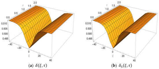
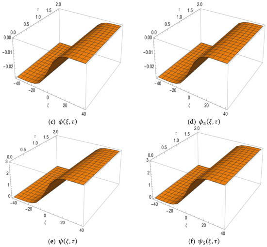
Figure 1. The exact solution and the fifth approximate LRPSM solution of HSC–KdV equations for the functions $\delta \left(\xi ,\tau \right), \varphi \left(\xi ,\tau \right)$, and $\psi \left(\xi ,\tau \right)$ at $\tau \in \left[0,2\right], \xi \in \left[-40,40\right],$ and $\alpha =1$.

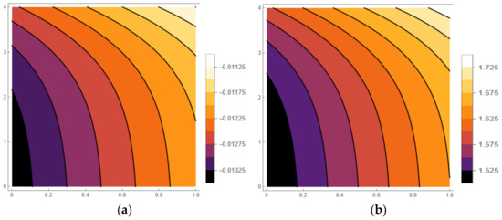
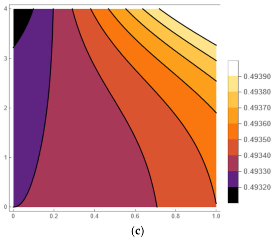
Figure 2. The contour graph of the approximate solutions (a) $\delta \left(\xi ,\tau \right),$(b) $\varphi \left(\xi ,\tau \right),$ and (c) $\psi \left(\xi ,\tau \right)$ for HSC–KdV equation at $\tau \in \left[0,4\right], \xi \in \left[0,1\right],$ and $\alpha =1$.

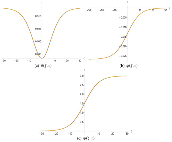
Figure 3. The graph of the 5th LRPSM solutions $\delta \left(\xi ,\tau \right), \varphi \left(\xi ,\tau \right),$ and $\psi \left(\xi ,\tau \right)$ for HSC–KdV equations at $\tau =0.1,\tau =1,\tau =0.1,\tau =3, \xi \in \left[-30,30\right],$ and $\alpha =1$.

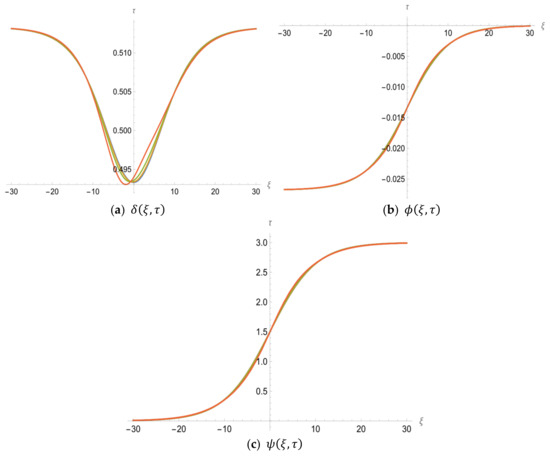
Figure 4. The graph of the 5th LRPSM solutions $\delta \left(\xi ,\tau \right), \varphi \left(\xi ,\tau \right),$ and $\psi \left(\xi ,\tau \right)$ for HSC–KdV equation at $\tau =0.1,\tau =1,\tau =2,\tau =3, \xi \in \left[-30,30\right],$ and $\alpha =1$.

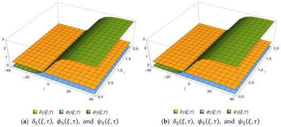
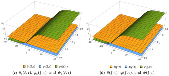
Figure 5. The 3D surface plot of the 10th approximate solutions of $u_1, u_2$, and $u_3$ at various values of $\alpha$ and $t=0.5$ and $\zeta =3$ for the problem in Example 4.3; (a) $\alpha =0.6$, (b) $\alpha =0.8$, (c) $\alpha =1$, (d) $\alpha =1$ (exact solutions).

5. Conclusions

This paper introduces a new series solution of the coupled Hirota–Satsuma and KdV equations and provides a general term of the solution. We applied the LRPSM to investigate the solution and obtained a general formula of the series solution for the target equations. We showed the efficiency and applicability of the method by introducing a numerical application and compared our results to the exact ones in the integer case. We analyzed the outcomes and sketched the solutions with different values for the variables and the fractional order. In the future, we intend to solve more physical problems with the LRPSM and compare the outcomes to those obtained by other numerical methods.

As a result of our research, we conclude the following:

• LRPSM is a powerful method for solving systems of fractional partial differential equations.
• LRPSM is a simple technique that could provide many terms of the obtained series solution.
• In comparison to other numerical methods, LRPSM needs less computation, without requiring linearization, discretization, or differentiation.
• The only disadvantage of the presented method is the Laplace transform step in the event that one the functions in the discussed problem is not of exponential order.

References

- Baleanu, D.; Diethelm, K.; Scalas, E.; Trujillo, J.J. Fractional Calculus: Models and Numerical Methods; World Scientific: Singapore, 2012; Volume 3. [Google Scholar]
- Petráš, I. Fractional-Order Nonlinear Systems: Modeling, Analysis and Simulation; Springer Science & Business Media: New York, NY, USA, 2011. [Google Scholar]
- Al-khateeb, A.; Zureigat, H.; Ala’yed, O.; Bawaneh, S. Ulam–Hyers Stability and Uniqueness for Nonlinear Sequential Fractional Differential Equations Involving Integral Boundary Conditions. Fractal Fract. 2021, 5, 235. [Google Scholar] [CrossRef]
- Kilbas, A.A.; Srivastava, H.M.; Trujillo, J.J. Theory and Applications of Fractional Differential Equations; Elsevier Science: Amsterdam, The Netherlands, 2006; Volume 204. [Google Scholar]
- Choo, K.Y.; Muniandy, S.V.; Woon, K.L.; Gan, M.T.; Ong, D.S. Modeling anomalous charge carrier transport in disordered organic semiconductors using the fractional drift-diffusion equation. Org. Electron. 2017, 41, 157–165. [Google Scholar] [CrossRef]
- Abbas, M.; Rizvi, A.A.; Naqvi, Q.A. Fractional dual fields to the Maxwell equations for a line source buried in dielectric half space. Optik 2017, 129, 225–230. [Google Scholar] [CrossRef]
- Formato, A.; Ianniello, D.; Villecco, F.; Lenza, T.L.; Guida, D. Design optimization of the plough working surface by computerized mathematical model. Emir. J. Food Agric. 2017, 1, 36–44. [Google Scholar] [CrossRef]
- Tariq, H.; Akram, G. New approach for exact solutions of time fractional Cahn-Allen equation and time fractional Phi-4 equation. Phys. A Stat. Mech. Appl. 2017, 473, 352–362. [Google Scholar] [CrossRef]
- Pellegrino, A.; Villecco, F. Design optimization of a natural gas substation with intensification of the energy cycle. Math. Probl. Eng. 2010, 2010, 294102. [Google Scholar] [CrossRef]
- Wang, L.; Sun, D.A.; Li, P.; Xie, Y. Semi-analytical solution for one-dimensional consolidation of fractional derivative viscoelastic saturated soils. Comput. Geotech. 2017, 83, 30–39. [Google Scholar] [CrossRef]
- Oskouie, M.F.; Ansari, R. Linear and nonlinear vibrations of fractional viscoelastic Timoshenko nanobeams considering surface energy effects. Appl. Math. Model. 2017, 43, 337–350. [Google Scholar] [CrossRef]
- Mohyud-Din, S.T.; Noor, M.A.; Noor, K.I.; Hosseini, M.M. Variational iteration method for re-formulated partial differential equations. Int. J. Nonlinear Sci. Numer. Simul. 2010, 11, 87–92. [Google Scholar] [CrossRef]
- Odibat, Z.M.; Kumar, S.; Shawagfeh, N.; Alsaedi, A.; Hayat, T. A study on the convergence conditions of generalized differential transform method. Math. Methods Appl. Sci. 2017, 40, 40–48. [Google Scholar] [CrossRef]
- Unal, E.; Gokdogan, A. Solution of conformable fractional ordinary differential equations via differential transform method. Optik 2017, 128, 264–273. [Google Scholar] [CrossRef]
- Shah, K.; Singh, T.; Kilicman, A. Combination of integral and projected differential transform methods for time-fractional gas dynamics equations. Ain. Shams. Eng. J. 2017, 9, 1683–1688. [Google Scholar] [CrossRef]
- Goswami, P.; Alqahtani, R.T. On the solution of local fractional differential equations using local fractional Laplace variational iteration method. Math. Probl. Eng. 2016, 2016, 9672314. [Google Scholar] [CrossRef]
- Jafari, H.; Jassim, H.K. Numerical solutions of telegraph and laplace equations on cantor sets using local fractional Laplace decomposition method. Int. J. Adv. Appl. Math. Mech. 2015, 2, 144–151. [Google Scholar]
- Ma, H.C.; Yao, D.D.; Peng, X.F. Exact solutions of non-linear fractional partial differential equations by fractional sub-equation method. Therm. Sci. 2015, 19, 1239–1244. [Google Scholar] [CrossRef]
- Feng, D.; Li, K. Exact traveling wave solutions for a generalized Hirota-Satsuma coupled KdV equation by Fan sub-equation method. Phys. Lett. A 2011, 375, 2201–2210. [Google Scholar] [CrossRef]
- Javeed, S.; Baleanu, D.; Waheed, A.; Shaukat Khan, M.; Affan, H. Analysis of Homotopy Perturbation Method for Solving Fractional Order Differential Equations. Mathematics 2019, 7, 40. [Google Scholar] [CrossRef]
- Mohyud-Din, S.T.; Noor, M.A.; Noor, K.I. Some relatively new techniques for nonlinear problems. Math. Probl. Eng. 2009, 2009, 234849. [Google Scholar] [CrossRef]
- Bekir, A.; Kaplan, M. Exponential rational function method for solving nonlinear equations arising in various physical models. Chin. J. Phys. 2016, 54, 365–370. [Google Scholar] [CrossRef]
- Noor, M.A.; Mohyud-Din, S.T.; Waheed, A.; Al-Said, E.A. Exp-function method for traveling wave solutions of nonlinear evolution equations. Appl. Math. Comput. 2010, 216, 477–483. [Google Scholar] [CrossRef]
- Pandir, Y.; Gurefe, Y.; Misirli, E. The extended trial equation method for some time fractional differential equations. Discrete Dyn. Nat. Soc. 2013, 2013, 491359. [Google Scholar] [CrossRef]
- Burqan, A.; Saadeh, R.; Qazza, A.; Momani, S. ARA-Residual Power Series Method for Solving Partial Fractional Differential Equations. Alex. Eng. J. 2023, 62, 47–62. [Google Scholar]
- Qazza, A.; Burqan, A.; Saadeh, R.; Khalil, R. Applications on Double ARA–Sumudu Transform in Solving Fractional Partial Differential Equations. Symmetry 2022, 14, 1817. [Google Scholar] [CrossRef]
- Saadeh, R. Numerical algorithm to solve a coupled system of fractional order using a novel reproducing kernel method. Alex. Eng. J. 2021, 60, 4583–4591. [Google Scholar] [CrossRef]
- Berz, M. The method of power series tracking for the mathematical description of beam dynamics. Nucl. Instrum. Methods Phys. Res. A 1987, 258, 431–436. [Google Scholar] [CrossRef]
- El-Ajou, A. Adapting the Laplace transform to create solitary solutions for the nonlinear time-fractional dispersive PDEs via a new approach. Eur. Phys. J. Plus 2021, 136, 229. [Google Scholar] [CrossRef]
- Eriqat, T.; El-Ajou, A.; Oqielat, M.N.; Al-Zhour, Z.; Momani, S. A new attractive analytic approach for solutions of linear and nonlinear neutral fractional pantograph equations. Chaos Solitons Fractals 2020, 138, 109957. [Google Scholar] [CrossRef]
- Kazem, S. Exact solution of some linear fractional differential equations by Laplace transform. Int. J. Nonlinear Sci. 2013, 16, 3–11. [Google Scholar]
- Saadeh, R.; Burqan, A.; El-Ajou, A. Reliable solutions to fractional Lane-Emden equations via Laplace transform and residual error function. Alex. Eng. J. 2022, 61, 10551–10562. [Google Scholar] [CrossRef]
- Saadeh, R.; Qazza, A.; Amawi, K. A New Approach Using Integral Transform to Solve Cancer Models. Fractal Fract. 2022, 6, 490. [Google Scholar] [CrossRef]
- Alderremy, A.A.; Shah, R.; Iqbal, N.; Aly, S.; Nonlaopon, K. Fractional Series Solution Construction for Nonlinear Fractional Reaction-Diffusion Brusselator Model Utilizing Laplace Residual Power Series. Symmetry 2022, 14, 1944. [Google Scholar] [CrossRef]
- Ali, A.T.; Khater, M.M.; Attia, R.A.; Abdel-Aty, A.H.; Lu, D. Abundant numerical and analytical solutions of the generalized formula of Hirota-Satsuma coupled KdV system. Chaos Solitons Fractals 2020, 131, 109473. [Google Scholar] [CrossRef]
- Diethelm, K. A fractional calculus based model for the simulation of an outbreak of dengue fever. Nonlinear Dyn. 2013, 71, 613–619. [Google Scholar] [CrossRef]
- Veeresha, P.; Prakasha, D.G.; Baskonus, H.M. Novel simulations to the time-fractional Fisher’s equation. Math. Sci. 2019, 13, 33. [Google Scholar] [CrossRef]
Publisher’s Note: MDPI stays neutral with regard to jurisdictional claims in published maps and institutional affiliations. |
© 2022 by the authors. Licensee MDPI, Basel, Switzerland. This article is an open access article distributed under the terms and conditions of the Creative Commons Attribution (CC BY) license (https://creativecommons.org/licenses/by/4.0/).