An Approach for Numerical Solutions of Caputo–Hadamard Uncertain Fractional Differential Equations

Abstract

This paper is devoted to investigating a numerical scheme for solving the Caputo–Hadamard uncertain fractional differential equations (UFDEs) arising from nonlinear uncertain dynamic systems. In our approach, we define an $\alpha$-path, which is a link between a Caputo–Hadamard UFDE and a Caputo–Hadamard fractional differential equation and is the inverse uncertainty distribution of a Caputo–Hadamard UFDE. Then, a formula for calculating the expected value of the Caputo–Hadamard UFDE is studied. With the help of the modified predictor–corrector method, some numerical algorithms for the inverse uncertainty distribution and the expected value of the solution of Caputo–Hadamard UFDEs are designed. Corresponding numerical examples are given to confirm the validity and accuracy of the proposed algorithms.

1. Introduction

In the real world, a system is commonly disturbed by noise. If the noise is described by stochastic factors, the tool of probability theory is usually used to deal with the system, which requires sufficient data and needs to ensure that the estimated probability distribution is very close to the real frequency. When lacking historical data on research problems, we can use the experience of experts in the relevant field to estimate the brief degree of the event happening. In order to rationally deal with the likelihood that something will happen, Liu [1] proposed the uncertainty theory in 2007 and perfected this theory in 2010 [2]. To describe the uncertain system more accurately, Liu [3,4] investigated uncertain processes and applied them to uncertain differential equations (UDEs). Then, Chen and Liu [5] proved the existence and uniqueness theorem of the solutions of UDEs and gave some analytic scheme.

In 1974, Oldham and Spanier [6] proposed fractional calculus, which received the attention of many scholars [7,8,9,10,11]. Since fractional differential equations (FDEs) can well describe a system with memory and heritability, they have been deeply studied in various fields, such as chaos, electrochemistry, rheology, and so on [12,13,14]. At present, the theoretical research on fractional calculus mainly discusses the Riemann–Liouville type and the Caputo type. While for some logarithmic problems, the Hadmard type and Caputo–Hadamard type are more appropriate, which were studied by Hadamard [15] and Jarad et al. [16], respectively. Subsequently, Kilbas [17] studied some basic properties of Hadamard type fractional differentiation and integration. Gohar et al. [18] studied the existence and uniqueness of the solutions of Caputo–Hadamard FDEs.

In order to make an uncertain system have the memory property, Zhu [19] incorporated the uncertainty into the FDE and defined the uncertain fractional differential equation (UFDE). Then, the analytic solutions for some special Riemann–Liouville and Caputo UFDEs were given. At the same time, Zhu [20] proved the existence and uniqueness theorem of solutions of UFDEs under Lipschitz and linear growth conditions. Subsequently, Lu et al. [21] extended the definitions of Riemann–Liouville and Caputo UFDEs from order $p\in (0,1)$ to order $p>0$. Mohammed et al. [22] considered the existence and uniqueness of the solutions of Riemann–Liouville uncertain fractional backward difference equations. Liu et al. [23] gave the definition of Caputo–Hadamard UFDEs and proved the existence and uniqueness theorem of their solutions.

For many nonlinear differential equations, it is difficult to obtain an analytic solution, while in reality, they are extensively used for describing important physical phenomena. Rashid et al. [24] studied nonlinear time-fractional partial differential equations arising in physical systems involving the natural decomposition method. Khan et al. [25] investigated space–time fractional diffusion equations to describing anomalous diffusion. Studying numerical algorithms has become a hot research topic. In 2013, Yao and Chen [26] proposed the concept of the $\alpha$-path, establishing the connection between UDEs and ODEs. Gao [27] designed a new numerical algorithm for solving UDEs by the Milne method. Wang et al. [28] presented a numerical algorithm for solving UDEs via the Adams–Simpson method. Diethelm et al. [29,30] studied the Adams type predictor–corrector method suitable for solving numerical solutions of FDEs. Lu and Zhu [31] introduced a numerical method for solving UFDEs based on the predictor–corrector method. Gohar et al. [32] gave the modified predictor–corrector method applied to the Caputo–Hadamard derivative. However, there is no research on numerical algorithms for Caputo–Hadamard UFDEs.

In this paper, we mainly discuss the numerical algorithm for solving the nonlinear Caputo–Hadamard UFDEs. The rest of this paper is arranged as follows: in Section 2, we introduce some basic concepts and conclusions that are used later. In Section 3, the concept of the $\alpha$-path is proposed, and an important theorem is proved on the basis of the $\alpha$-path. In Section 4, an expected value formula of the solution with respect to the Caputo–Hadamard UFDE is given. In Section 5, numerical algorithms for computing the inverse uncertainty distribution and expected value are presented. In Section 6, some numerical examples are given to verify the effectiveness and accuracy of the proposed algorithm. Section 7 is the conclusion of this paper.

2. Preliminary

For preparing the later study about the numerical solutions of Caputo–Hadamard UFDEs, some basic notions and conclusions of the uncertainty theory, such as an uncertain measure, uncertain variable, uncertainty distribution, uncertain differential equation, excepted value, etc., can be seen in [1,2,27,28]. An uncertain process $C_t$ is said to be a Liu process if (i) $C_0=0$ and almost all sample paths are Lipschitz continuous, (ii) $C_t$ has stationary and independent increments and (iii) every increment $C_{s+t}-C_s$ is a normal uncertain variable with expected value zero and variance $t^2$. For an uncertain variable $\xi$ with a regular distribution $\mathsf{\Phi }\left(x\right)$, the expected value of $\xi$ is $E\left[\xi \right]={\int }_0^1{\mathsf{\Phi }}^{-1}\left(\alpha \right)\mathrm{d}\alpha$.

In this section, we introduce some concepts and results of Caputo–Hadamard UFDEs.

Definition 1

([23]). Consider $n-1<p\le n$ having $n\in {\mathrm{N}}^{+}$ with $\delta =t\frac{\mathrm{d}}{\mathrm{d}t}$, $C_t$ a Liu process and f and g two continuous functions on $[a,\infty )\times \mathrm{R}\to \mathrm{R}$. The Caputo–Hadamard UFDE with initial conditions is defined as

$$\left\{\begin{array}{c}{}^{CH}{\mathcal{D}}_{a^{+}}^p{X}_t=f\left(t,X_t\right)+g\left(t,X_t\right)\frac{\mathrm{d}{C}_t}{\mathrm{d}t},t\ge a>0,\hfill \\ {\left.{\delta }^k{X}_t\right|}_{t=a}=x_k,k=0,1,\dots ,n-1.\hfill \end{array}\right.$$

(1)

The solution of (1) is an uncertain process $X_t$ with the following integral equation

$$\begin{array}{cc}\hfill X_t=& \sum _{k=0}^{n-1}\frac{{\left(log\frac{t}{a}\right)}^k}{\mathsf{\Gamma }(k+1)}{x}_k+{\mathcal{J}}_{a^{+}}^{p}f\left(t,X_t\right)+{\mathcal{J}}_{a^{+}}^p\left(g\left(t,X_t\right)\frac{\mathrm{d}{C}_t}{\mathrm{d}t}\right)\hfill \\ \hfill =& \sum _{k=0}^{n-1}\frac{{\left(log\frac{t}{a}\right)}^k}{\mathsf{\Gamma }(k+1)}{x}_k+\frac{1}{\mathsf{\Gamma }\left(p\right)}{\int }_a^t{\left(log\frac{t}{s}\right)}^{p-1}f\left(s,X_s\right)\frac{\mathrm{d}s}{s}\hfill \\ \hfill & +\frac{1}{\mathsf{\Gamma }\left(p\right)}{\int }_a^t{\left(log\frac{t}{s}\right)}^{p-1}g\left(s,X_s\right)\frac{\mathrm{d}{C}_s}{s}.\hfill \end{array}$$

(2)

Lemma 1

([23]). (Existence and uniqueness) If functions $f(t,x)$ and $g(t,x)$ in (1) satisfying the Lipschitz condition

$$\left|f\right(t,x)-f(t,y\left)\right|+\left|g\right(t,x)-g(t,y\left)\right|\le L|x-y|,\forall x,y\in \mathrm{R},t\ge a>0$$

(3)

and the linear growth condition

$$\left|f\right(t,x\left)\right|+\left|g\right(t,x\left)\right|\le L(1+|x\left|\right),\forall x\in \mathrm{R},t\ge a>0,$$

(4)

where L is a positive constant, then the Caputo–Hadamard UFDE (1) has a unique solution almost surely.

Some definitions of fractional calculus and FDEs can be seen in [7,8].

Remark 1.(i) For any function $f\left(t\right)$, the Hadamard integral of order $p>0$ is defined by

$${\mathcal{J}}_{a^{+}}^{p}f\left(t\right)=\frac{1}{\mathsf{\Gamma }\left(p\right)}{\int }_a^t{\left(log\frac{t}{s}\right)}^{p-1}f\left(s\right)\frac{\mathrm{d}s}{s},a<t.$$

(5)

(ii) For $n-1<p\le n$ having $n\in {\mathrm{N}}^{+}$ with $\delta =t\frac{\mathrm{d}}{\mathrm{d}t}$ and ${\delta }^n=\delta ·{\delta }^{n-1}$, the Caputo–Hadamard derivative of order $p>0$ for a function $f\left(t\right)$ is defined by

$${}^{CH}{\mathcal{D}}_{a^{+}}^{p}f\left(t\right)=\frac{1}{\mathsf{\Gamma }(n-p)}{\int }_a^t{\left(log\frac{t}{s}\right)}^{n-p-1}{\delta }^{n}f\left(s\right)\frac{\mathrm{d}s}{s},a<t,$$

(6)

where $n-1<p\le n\in {\mathrm{N}}^{+}$, $\delta =t\frac{\mathrm{d}}{\mathrm{d}t}$ and ${\delta }^n=\delta ·{\delta }^{n-1}.$

Lemma 2

([33]). For any continuous functions $f(t,x),F(t,x):[a,T]\times \mathrm{R}\to \mathrm{R}$ satisfying

$$f(t,x)\le F(t,x),(t,x)\in [a,T]\times \mathrm{R}.$$

(7)

and $0\le n-1<p\le n\in {\mathrm{N}}^{+}$, $x=u\left(t\right)$ and $x=v\left(t\right)$ are solutions of

$$\left(E_3\right){}^{CH}{\mathcal{D}}_{a^{+}}^{p}x=f(t,x),{\left.x^{\left(k\right)}\left(t\right)\right|}_{t=a}=x_k,k=0,1,\dots ,n-1,$$

(8)

$$\left(E_4\right){}^{CH}{\mathcal{D}}_{a^{+}}^{p}x=F(t,x),{\left.x^{\left(k\right)}\left(t\right)\right|}_{t=a}=x_k,k=0,1,\dots ,n-1,$$

(9)

respectively. If inequality (7) is strict, then $u\left(t\right)<v\left(t\right),\forall t\in (a,T]$. If $\left(E_3\right)$ and $\left(E_4\right)$ have a unique solution, respectively, then $u\left(t\right)$ ≤ $v\left(t\right)$, $\forall t\in (a,T]$.

3. The $\mathbf{\alpha }$-Path of Caputo–Hadamard UFDEs

In this section, the concept of the $\alpha$-path of Caputo–Hadamard UFDEs is proposed, which is essentially the solution of a Caputo–Hadamard FDE.

Definition 2.

For $n-1<p\le n$ having $n\in {\mathrm{N}}^{+}$ with $\delta =t\frac{\mathrm{d}}{\mathrm{d}t}$, $C_t$ a Liu process and f and g two continuous functions on $[a,\infty )\times \mathrm{R}\to \mathrm{R}$, the Caputo–Hadamard UFDE subject to the initial conditions

$$\left\{\begin{array}{c}{}^{CH}{\mathcal{D}}_{a^{+}}^p{X}_t=f\left(t,X_t\right)+g\left(t,X_t\right)\frac{\mathrm{d}{C}_t}{\mathrm{d}t},T\ge t\ge a>0,\hfill \\ {\left.{\delta }^k{X}_t\right|}_{t=a}=x_k,k=0,1,\dots ,n-1\hfill \end{array}\right.$$

(10)

is said to have an α-path $X_t^{\alpha }$ which is a function of t and solves the corresponding Caputo–Hadamard FDE with initial conditions

$$\left\{\begin{array}{c}{}^{CH}{\mathcal{D}}_{a^{+}}^p{X}_t=f\left(t,X_t\right)+\left|g\left(t,X_t\right)\right|{\mathsf{\Phi }}^{-1}\left(\alpha \right),T\ge t\ge a>0,\hfill \\ {\left.{\delta }^k{X}_t\right|}_{t=a}=x_k,k=0,1,\dots ,n-1,\hfill \end{array}\right.$$

(11)

where $\alpha \in (0,1)$ and ${\mathsf{\Phi }}^{-1}\left(\alpha \right)$ is the inverse standard normal uncertainty distribution, i.e.,

$${\mathsf{\Phi }}^{-1}\left(\alpha \right)=\frac{\sqrt{3}}{\pi }ln\frac{\alpha }{1-\alpha },0<\alpha <1.$$

(12)

Here are some examples to illustrate Definition 2.

Example 1.

For any $0<p\le 1,u,v>-1$, the Caputo–Hadamard UFDE subject to the initial condition

$$\left\{\begin{array}{c}{}^{CH}{\mathcal{D}}_{1^{+}}^p{X}_t=a{\left(logt\right)}^u+b{\left(logt\right)}^v\frac{\mathrm{d}{C}_t}{\mathrm{d}t},t\in [1,T],\hfill \\ {\left.X_t\right|}_{t=1}=x_0\hfill \end{array}\right.$$

(13)

has an $\alpha$-path which is a solution of the following Caputo–Hadamard FDE with initial condition

$$\left\{\begin{array}{c}{}^{CH}{\mathcal{D}}_{1^{+}}^p{X}_t=a{\left(logt\right)}^u+\left|b{\left(logt\right)}^v\right|{\mathsf{\Phi }}^{-1}\left(\alpha \right),t\in [1,T],\hfill \\ {\left.X_t\right|}_{t=1}=x_0,\hfill \end{array}\right.$$

(14)

that is,

$$\begin{array}{c}\hfill X_t^{\alpha }=x_0+\frac{a\mathsf{\Gamma }(u+1)}{\mathsf{\Gamma }(p+u+1)}{(logt)}^{p+u}+\frac{\left|b\right|\mathsf{\Gamma }(v+1)}{\mathsf{\Gamma }(p+v+1)}{(logt)}^{p+v}\frac{\sqrt{3}}{\pi }ln\frac{\alpha }{1-\alpha }.\end{array}$$

(15)

Example 2.

For any $0<p\le 1$, $u,v>0$, the Caputo–Hadamard UFDE subject to the initial condition

$$\left\{\begin{array}{c}{}^{CH}{\mathcal{D}}_{1^{+}}^p{X}_t=a{t}^u+b{t}^v\frac{\mathrm{d}{C}_t}{\mathrm{d}t},t\in [1,T],\hfill \\ {\left.X_t\right|}_{t=1}=x_0\hfill \end{array}\right.$$

(16)

has an $\alpha$-path which is a solution of the following Caputo–Hadamard FDE with initial condition

$$\left\{\begin{array}{c}{}^{CH}{\mathcal{D}}_{1^{+}}^p{X}_t=a{t}^u+\left|b{t}^v\right|{\mathsf{\Phi }}^{-1}\left(\alpha \right),t\in [1,T],\hfill \\ {\left.X_t\right|}_{t=1}=x_0,\hfill \end{array}\right.$$

(17)

that is,

$$X_t^{\alpha }=x_0+a{u}^{-p}{t}^u+\left|b\right|v^{-p}{t}^v\frac{\sqrt{3}}{\pi }ln\frac{\alpha }{1-\alpha }.$$

(18)

Example 3.

For any $0<p\le 1,v>-1$, the Caputo–Hadamard UFDE subject to the initial condition

$$\left\{\begin{array}{c}{}^{CH}{\mathcal{D}}_{1^{+}}^p{X}_t=a{X}_t+b{(logt)}^v\frac{\mathrm{d}{C}_t}{\mathrm{d}t},t\in [1,T],\hfill \\ {\left.X_t\right|}_{t=1}=x_0\hfill \end{array}\right.$$

(19)

has an $\alpha$-path which is a solution of the following Caputo–Hadamard FDE with initial condition

$$\left\{\begin{array}{c}{}^{CH}{\mathcal{D}}_{1^{+}}^p{X}_t=a{X}_t+b{(logt)}^v{\mathsf{\Phi }}^{-1}\left(\alpha \right),t\in [1,T],\hfill \\ {\left.X_t\right|}_{t=1}=x_0,\hfill \end{array}\right.$$

(20)

that is,

$$X_t^{\alpha }=x_0{E}_{p,1}\left(a{\left(logt\right)}^p\right)+\left|b\right|\mathsf{\Gamma }(v+1){(logt)}^{p+v}{E}_{p,p+v+1}\left(a{\left(logt\right)}^p\right)\frac{\sqrt{3}}{\pi }ln\frac{\alpha }{1-\alpha }.$$

(21)

Next, we introduce an important theorem, which establishes the relation between a Caputo–Hadamard UFDE and a Caputo–Hadamard FDE.

Theorem 1.

For $n-1<p\le n$ having $n\in {\mathrm{N}}^{+}$, $C_t$ a Liu process and f and g two continuous functions on $[a,\infty )\times \mathrm{R}\to \mathrm{R}$, let $X_t$ and $X_t^{\alpha }$ be the unique solution and α-path of the Caputo–Hadamard UFDE (10), respectively. Then, we have

$$\mathcal{M}\{X_t\le X_t^{\alpha },a.e.t\in (a,T]\}=\alpha$$

(22)

and

$$\mathcal{M}\{X_t>X_t^{\alpha },a.e.t\in (a,T]\}=1-\alpha .$$

(23)

Proof. 

For any $x\in \mathrm{R}$ and $\alpha \in (0,1)$, divide the time interval $(a,T]$ into two disjoint subsets

$${\mathsf{\Omega }}^{+}=\{t\in (a,T]g(t,x)\ge 0\},{\mathsf{\Omega }}^{-}=\{t\in (a,T]g(t,x)<0\}.$$

It is easy to get that ${\mathsf{\Omega }}^{+}\cap {\mathsf{\Omega }}^{-}=\varphi$ and ${\mathsf{\Omega }}^{+}\cup {\mathsf{\Omega }}^{-}=(a,T]$. Denote

$${\mathsf{\Lambda }}_1^{+}=\{\gamma \frac{\mathrm{d}{C}_t}{\mathrm{d}t}\le {\mathsf{\Phi }}^{-1}\left(\alpha \right),a.e.t\in {\mathsf{\Omega }}^{+}\},{\mathsf{\Lambda }}_1^{-}=\{\gamma \frac{\mathrm{d}{C}_t}{\mathrm{d}t}\ge {\mathsf{\Phi }}^{-1}(1-\alpha ),a.e.t\in {\mathsf{\Omega }}^{-}\},$$

where ${\mathsf{\Phi }}^{-1}\left(\alpha \right)$ is the inverse uncertainty distribution of a standard normal uncertain variable. Considering that $C_t$ is a Liu process with independent increments and ${\mathsf{\Omega }}^{+}\cap {\mathsf{\Omega }}^{-}=\varphi$, we get

$$\mathcal{M}\left\{{\mathsf{\Lambda }}_1^{+}\right\}=\alpha ,\mathcal{M}\left\{{\mathsf{\Lambda }}_1^{-}\right\}=\alpha ,\mathcal{M}\{{\mathsf{\Lambda }}_1^{+}\cap {\mathsf{\Lambda }}_1^{-}\}=\mathsf{\alpha }.$$

For each $\gamma \in {\mathsf{\Lambda }}_1^{+}\cap {\mathsf{\Lambda }}_1^{-}$ and a.e. $t\in (a,T]$, we have

$$g(t,x\left(t\right))\frac{\mathrm{d}{C}_t}{\mathrm{d}t}\le \left|g(t,x(t\left)\right)\right|{\mathsf{\Phi }}^{-1}\left(\alpha \right).$$

Since $X_t$ and $X_t^{\alpha }$ are unique solutions to a Caputo–Hadamard UFDE (10) and a Caputo–Hadamard FDE (11), respectively. It follows from Lemma 2 that

$$X_t\left(\gamma \right)\le X_t^{\alpha }\left(\gamma \right),a.e.t\in (a,T].$$

Thus, we can get that

$${\mathsf{\Lambda }}_1^{+}\cap {\mathsf{\Lambda }}_1^{-}\subset \{X_t\le X_t^{\alpha },a.e.t\in (a,T]\}.$$

Then, for all $t\in (a,T]$, we have

$$\mathcal{M}\{X_t\le X_t^{\alpha },a.e.t\in (a,T]\}\ge \mathcal{M}\{{\mathsf{\Lambda }}_1^{+}\cap {\mathsf{\Lambda }}_1^{-}\}=\alpha .$$

(24)

Denote

$${\mathsf{\Lambda }}_2^{+}=\{\gamma \frac{\mathrm{d}{C}_t}{\mathrm{d}t}>{\mathsf{\Phi }}^{-1}\left(\alpha \right),a.e.t\in {\mathsf{\Omega }}^{+}\},{\mathsf{\Lambda }}_2^{-}=\{\gamma \frac{\mathrm{d}{C}_t}{\mathrm{d}t}<{\mathsf{\Phi }}^{-1}(1-\alpha ),a.e.t\in {\mathsf{\Omega }}^{-}\}.$$

Similarly, we have

$$\mathcal{M}\left\{{\mathsf{\Lambda }}_2^{+}\right\}=1-\alpha ,\mathcal{M}\left\{{\mathsf{\Lambda }}_2^{-}\right\}=1-\alpha ,\mathcal{M}\{{\mathsf{\Lambda }}_2^{+}\cap {\mathsf{\Lambda }}_2^{-}\}=1-\alpha .$$

Then, for all $\gamma \in {\mathsf{\Lambda }}_2^{+}\cap {\mathsf{\Lambda }}_2^{-}$ and $t\in (a,T]$, we have

$$g(t,x\left(t\right))\frac{\mathrm{d}{C}_t}{\mathrm{d}t}>\left|g(t,x(t\left)\right)\right|{\mathsf{\Phi }}^{-1}\left(\alpha \right)$$

It follows from Lemma 2 that

$$X_t\left(\gamma \right)>X_t^{\alpha }\left(\gamma \right),a.e.t\in (a,T].$$

Then, we have

$${\mathsf{\Lambda }}_2^{+}\cap {\mathsf{\Lambda }}_2^{-}\subset \{X_t>X_t^{\alpha },a.e.t\in (a,T]\}$$

and

$$\mathcal{M}\{X_t>X_t^{\alpha },\forall t\in (a,T]\}\ge \mathcal{M}\{{\mathsf{\Lambda }}_2^{+}\cap {\mathsf{\Lambda }}_2^{-}\}=1-\alpha .$$

(25)

It follows from the duality axiom in the uncertainty theory that

$$\mathcal{M}\{X_t\le X_t^{\alpha },a.e.t\in (a,T]\}+\mathcal{M}\{X_t\nleqq X_t^{\alpha },a.e.t\in (a,T]\}=1.$$

Since

$$\{X_t>X_t^{\alpha },a.e.t\in (a,T]\}\subset \{X_t\nleqq X_t^{\alpha },a.e.t\in (a,T]\}.$$

It follows from the monotonicity of the uncertain measure $\mathcal{M}$ that

$$\mathcal{M}\{X_t\le X_t^{\alpha },a.e.t\in (a,T]\}+\mathcal{M}\{X_t>X_t^{\alpha },a.e.t\in (a,T]\}\le 1.$$

(26)

Combining Equations (24)–(26), we have

$$\mathcal{M}\{X_t\le X_t^{\alpha },a.e.t\in (a,T]\}=\alpha ,\mathcal{M}\{X_t>X_t^{\alpha },a.e.t\in (a,T]\}=1-\alpha .$$

The proof ends.    □

Theorem 2.

For $n-1<p\le n$ having $n\in {\mathrm{N}}^{+}$, $C_t$ a Liu process and f and g two continuous functions on $[a,\infty )\times \mathrm{R}\to \mathrm{R}$, let $X_t$ and $X_t^{\alpha }$ be the unique solution and α-path of the Caputo–Hadamard UFDE (10), respectively. Then, $X_t$ has an inverse uncertainty distribution

$${\mathsf{\Psi }}_t^{-1}\left(\alpha \right)=X_t^{\alpha },a.e.t.$$

(27)

Proof. 

Since $\{X_s\le X_s^{\alpha },a.e.s\}\subset \{X_t\le X_t^{\alpha }\}$ and $\{X_s>X_s^{\alpha },a.e.s\}\subset \{X_t>X_t^{\alpha }\}$, a.e. t. According to Theorem 1 and the monotonicity of the uncertain measure $\mathcal{M}$, we have

$$\mathcal{M}\{X_t\le X_t^{\alpha }\}\ge \mathcal{M}\{X_s\le X_s^{\alpha },a.e.s\}=\alpha ,a.e.t.$$

(28)

and

$$\mathcal{M}\{X_t>X_t^{\alpha }\}\ge \mathcal{M}\{X_s>X_s^{\alpha },a.e.s\}=1-\alpha ,a.e.t.$$

(29)

Since $\{X_t\le X_t^{\alpha }\}$ and $\{X_t>X_t^{\alpha }\}$ are opposite, it follows from the duality axiom in the uncertainty theory that

$$\mathcal{M}\{X_t\le X_t^{\alpha }\}+\mathcal{M}\{X_t>X_t^{\alpha }\}=1.$$

(30)

Combining Equations (28)–(30), we have $\mathcal{M}\{X_t\le X_t^{\alpha }\}=\alpha$ a.e. $t\in (a,T]$. Thus, $X_t$ has an inverse uncertainty distribution ${\mathsf{\Psi }}_t^{-1}\left(\alpha \right)=X_t^{\alpha },a.e.t.$    □

Next, we use some examples to illustrate the validity of Theorem 2.

Example 4.

The Caputo–Hadamard UFDE (13) has a solution

$$X_t=x_0+\frac{a\mathsf{\Gamma }(u+1)}{\mathsf{\Gamma }(p+u+1)}{(logt)}^{p+u}+\frac{b}{\mathsf{\Gamma }\left(p\right)}{\int }_1^t{\left(log\frac{t}{s}\right)}^{p-1}{(logs)}^v\frac{\mathrm{d}{C}_s}{s}.$$

(31)

Solution (31) has an inverse uncertainty distribution

$${\mathsf{\Psi }}_t^{-1}\left(\alpha \right)=x_0+\frac{a\mathsf{\Gamma }(u+1)}{\mathsf{\Gamma }(p+u+1)}{(logt)}^{p+u}+\frac{\left|b\right|\mathsf{\Gamma }(v+1)}{\mathsf{\Gamma }(p+v+1)}{(logt)}^{p+v}\frac{\sqrt{3}}{\pi }ln\frac{\alpha }{1-\alpha },$$

(32)

that is also the $\alpha$-path of the Caputo–Hadamard UFDE (13).

Example 5.

The Caputo–Hadamard UFDE (16) has a solution

$$X_t=x_0+a{u}^{-p}{t}^u+b{\int }_0^t{\left(log\frac{t}{s}\right)}^{p-1}{s}^v\frac{\mathrm{d}{C}_s}{\mathrm{d}s}.$$

(33)

Solution (33) has an inverse uncertainty distribution

$${\mathsf{\Psi }}_t^{-1}\left(\alpha \right)=x_0+a{u}^{-p}{t}^u+\left|b\right|v^{-p}{t}^v\frac{\sqrt{3}}{\pi }ln\frac{\alpha }{1-\alpha },$$

(34)

that is also the $\alpha$-path of the Caputo–Hadamard UFDE (16).

Example 6.

The Caputo–Hadamard UFDE (19) has a solution

$$X_t=x_0{E}_{p,1}\left(a{\left(logt\right)}^p\right)+b{\int }_1^t{(log\frac{t}{s})}^{p-1}{E}_{p,p}(a{(log\frac{t}{s})}^p){(logt)}^v\frac{\mathrm{d}{C}_s}{\mathrm{d}s}.$$

(35)

Solution (35) has an inverse uncertainty distribution

$${\mathsf{\Psi }}_t^{-1}\left(\alpha \right)=x_0{E}_{p,1}\left(a{\left(logt\right)}^p\right)+\left|b\right|\mathsf{\Gamma }(v+1){\left(logt\right)}^{p+v}{E}_{p,p+v+1}\left(a{\left(logt\right)}^p\right)\frac{\sqrt{3}}{\pi }ln\frac{\alpha }{1-\alpha },$$

(36)

that is also the $\alpha$-path of the Caputo–Hadamard UFDE (19).

4. Expected Value of a Monotonic Function

In this section, we propose an expected value theorem for calculating the expected value of the solutions of Caputo–Hadamard UFDEs.

Theorem 3.

Let $p_i$$(i=1,2,\dots ,q)$ be real numbers with $0\le n_i-1<p_i\le n_i$, where $n_i$$(i=1,2,\dots ,q)$ is a positive integer. Let $f_i(t,x),g_i(t,x):[a,T]\times R\to R$$(i=1,2,\dots ,q)$ be continuous functions. Assume that $X_{i,t}$ and $X_{i,t}^{\alpha }$ are the solution and α-path of Caputo–Hadamard UFDEs with initial conditions

$$\left\{\begin{array}{c}{}^{CH}{\mathcal{D}}_{a^{+}}^{p_i}{X}_{i,t}=f_i\left(t,X_{i,t}\right)+g_i\left(t,X_{i,t}\right)\frac{\mathrm{d}{C}_{i,t}}{\mathrm{d}t},t\ge a>0,\hfill \\ {\left.{\delta }^k{X}_{i,t}\right|}_{t=a}=x_{ik},k=0,1,\dots ,n_i-1\hfill \end{array}\right.$$

(37)

for $i=1,2,\dots ,q$, where $C_{i,t}$$(i=1,2,\dots ,q)$ are independent Liu processes. Assume that the function $J\left(x_1,x_2,\dots ,x_q\right)$ is strictly increasing with respect to $x_1,x_2,\dots ,x_m$ and strictly decreasing with respect to $x_{m+1},x_{m+2},\dots ,x_q$. Then, the expected value of $J\left(x_1,x_2,\dots ,x_q\right)$ can be calculated by the integral

$$E\left[J(X_{1,t},X_{2,t},\dots ,X_{q,t})\right]={\int }_0^{1}J(X_{1,t}^{\alpha },X_{2,t}^{\alpha },\dots ,X_{m,t}^{\alpha },X_{m+1,t}^{1-\alpha },X_{m+2,t}^{1-\alpha },\dots ,X_{q,t}^{1-\alpha })\mathrm{d}\alpha .$$

(38)

Proof. 

According to Theorem 2, the inverse uncertainty distribution of the solution of a Caputo–Hadamard UFDE (37) is

$${\mathsf{\Psi }}_{i,t}^{-1}\left(\alpha \right)=X_{i,t}^{\alpha },a.e.t,i=1,2,\dots ,q.$$

(39)

Then, the inverse uncertainty distribution of the function $J(X_{1,t},X_{2,t},\dots ,X_{q,t})$ is

$${{\rm Y}}_t^{-1}\left(\alpha \right)=J(X_{1,t}^{\alpha },X_{2,t}^{\alpha },\dots ,X_{m,t}^{\alpha },X_{m+1,t}^{1-\alpha },X_{m+2,t}^{1-\alpha },\dots ,X_{q,t}^{1-\alpha }),a.e.t\in [a,T].$$

(40)

That is to say, the expected value of $J\left(x_1,x_2,\dots ,x_q\right)$ is

$$\begin{array}{cc}\hfill E\left[J(X_{1,t},X_{2,t},\dots ,X_{q,t})\right]& ={\int }_0^1{{\rm Y}}_t^{-1}\left(\alpha \right)\mathrm{d}\alpha \hfill \\ \hfill & ={\int }_0^{1}J(X_{1,t}^{\alpha },X_{2,t}^{\alpha },\dots ,X_{m,t}^{\alpha },X_{m+1,t}^{1-\alpha },X_{m+2,t}^{1-\alpha },\dots ,X_{q,t}^{1-\alpha })\mathrm{d}\alpha .\hfill \end{array}$$

(41)

The proof ends.    □

5. Numerical Algorithms for Caputo–Hadamard UFDE

For most Caputo–Hadamard UFDEs, it is difficult to obtain analytic solutions. When a Caputo–Hadamard UFDE is nonlinear, there may be no analytic solution. Thus, to propose a corresponding numerical algorithm for finding the numerical solution of a Caputo–Hadamard UFDE is required.

Based on the $\alpha$-path and the modified predictor–corrector method [32], an algorithm for solving the inverse uncertainty distribution of the solutions of Caputo–Hadamard UFDEs (1) is given in Algorithm 1.

Algorithm 1: Inverse uncertainty distribution of the solutions of Caputo–Hadamard UFDEs.

Step 1.    For $t\in [a,T]$, divide the interval $\left[a,t\right]$ into N parts. Let $h=(t-a)/N$ be the step length. Set $\alpha =0$ and the step length $\mathsf{\Delta }\alpha$. Step 2.    Update $\alpha \leftarrow \alpha +\mathsf{\Delta }\alpha$, $i\leftarrow i+1$. Step 3.    Applying the modified predictor–corrector method [32] to the grid $t_i=1+ih$, solve the following Caputo–Hadamard FDE with initial conditions $$\left\{\begin{array}{c}{}^{CH}{\mathcal{D}}_{a^{+}}^p{X}_t^{\alpha }=f\left(t,X_t\right)+\left|g\left(t,X_t\right)\right|{\mathsf{\Phi }}^{-1}\left(\alpha \right),\hfill \\ {\left.{\delta }^k{X}_t\right|}_{t=a}=x_k,k=0,1,\dots ,n-1\hfill \end{array}\right.$$    to get $X_{t_i}^{\alpha }$. Step 4.    Output ${\mathsf{\Psi }}_{t_i}^{-1}\left(\alpha \right)=X_{t_i}^{\alpha }$. Step 5.    If $\alpha +\mathsf{\Delta }\alpha <1$ and $t_i<t$, go back to Step 2. Step 6.    Output ${\mathsf{\Psi }}_t^{-1}\left(\alpha \right)=X_t^{\alpha }$.

    In particular, when $\mathsf{\Delta }\alpha =0.01$, we can get the 99-table as Table 1.

Table 1. Ninety-nine-table.

$\alpha$	0.01	0.02	⋯	0.99
$X_t^{\alpha }$	$X_t^{0.01}$	$X_t^{0.02}$	⋯	$X_t^{0.99}$

According to Theorem 3, the expected value can be calculated by the integral equation

$$E\left[J\left(X_t\right)\right]={\int }_0^{1}J\left(X_t^{\alpha }\right)d\alpha .$$

(42)

When the above integral is an improper integral, we cannot operate the integral at the improper points. Thus, let the small enough positive number $ϵ$ such that ${\int }_0^{1}J\left(X_t^{\alpha }\right)d\alpha ={lim}_{ϵ\to 0}{\int }_{ϵ}^{1-ϵ}J\left(X_t^{\alpha }\right)d\alpha$. We apply Simpson’s rule to the above integral and the expected value of the strictly monotonic function $J\left(X_t\right)$ is computed by Algorithm 2.

Algorithm 2: Expected value of the solution of a Caputo–Hadamard UFDE.

Step 1.    For $t\in \left[a,T\right]$, give a small error $ϵ>0$. Let $\alpha =0$, set the step length $\mathsf{\Delta }\alpha =\frac{1}{M}$, where M is an even number. Step 2.    For each ${\alpha }_i=\mathsf{\Delta }\alpha ·i$$(i=1,2,\dots ,M-1)$, we can obtain $X_t^{ϵ}$, $X_t^{1-ϵ}$ and $X_t^{{\alpha }_i}$ by Algorithm 1. Step 3.    Apply Simpson’s rule to calculate the expected value of the strictly monotonic function $J\left(X_t\right)$. That is, $$E\left[J\left(X_t\right)\right]=\frac{\mathsf{\Delta }\alpha }{3}\left[J\left(X_t^{\epsilon }\right)+2\sum _{i=1}^{M-1}J\left(X_t^{{\alpha }_i}\right)+2\sum _{i=1}^{M/2}J\left(X_t^{{\alpha }_{2i-1}}\right)+J\left(X_t^{1-\epsilon }\right)\right].$$

6. Numerical Experiments

In this section, first, we analyze an example when the analytic solution can be obtained and compare the inverse uncertainty distribution of the numerical solution and the analytic solution to illustrate the accuracy of the proposed algorithms.

Example 7.

Let $1<p\le 2$; the following Caputo–Hadamard UFDE with initial conditions is considered:

$$\left\{\begin{array}{c}{}^{CH}{\mathcal{D}}_{1^{+}}^p{X}_t=a{\left(logt\right)}^u+b{\left(logt\right)}^v\frac{\mathrm{d}{C}_t}{\mathrm{d}t},t\in [1,T],\hfill \\ {\left.X_t\right|}_{t=1}=x_0,{\left.\delta X_t\right|}_{t=1}=x_1,\hfill \end{array}\right.$$

(43)

where the solution $X_t$ of (43) has an inverse uncertainty distribution

$$\begin{array}{cc}\hfill {\mathsf{\Psi }}_t^{-1}\left(\alpha \right)=& x_0+x_1(logt)+\frac{a\mathsf{\Gamma }(u+1)}{\mathsf{\Gamma }(p+u+1)}{(logt)}^{p+u}\hfill \\ & +\frac{\left|b\right|\mathsf{\Gamma }(v+1)}{\mathsf{\Gamma }(p+v+1)}{(logt)}^{p+v}\frac{\sqrt{3}}{\pi }ln\frac{\alpha }{1-\alpha }\hfill \end{array}$$

(44)

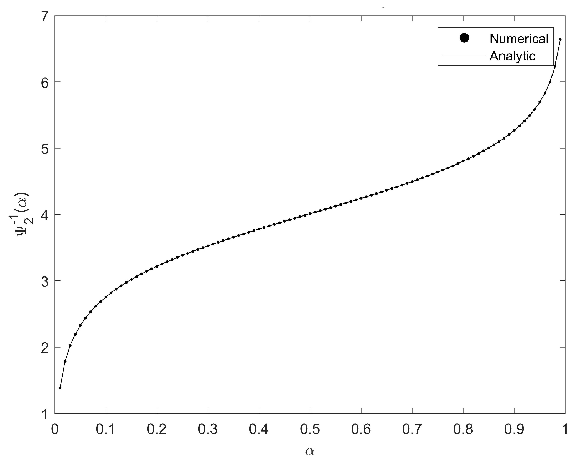
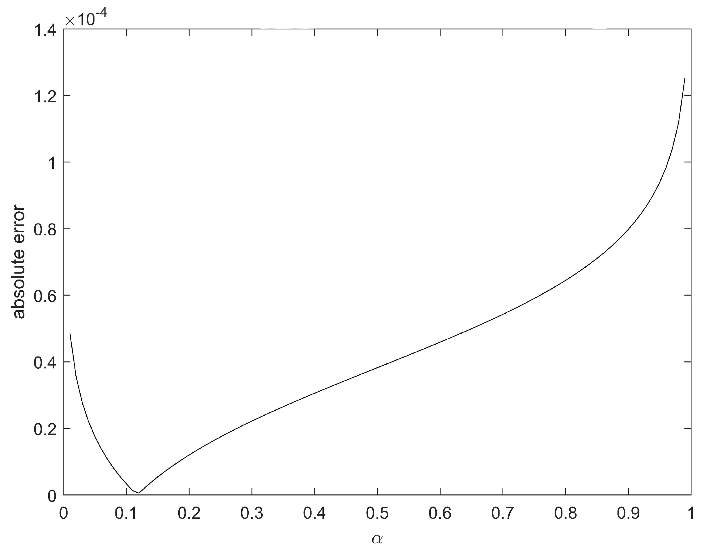
by Theorem 2. We choose the parameters as $p=1.6$, $a=6$, $b=10$, $u=2$, $v=1$ and $T=2$. Let the initial conditions $x_0=1$, $x_1=4$ and the step length $h=0.01$, $N=100$ and $\mathsf{\Delta }\alpha =0.01$. The inverse uncertainty distributions of the numerical solution and the analytic solution are obtained by Algorithm 1 and Equation (44), respectively, as shown in Figure 1. The absolute error between the inverse uncertainty distribution of the numerical and analytic solutions is less than $1.4\times {10}^{-4}$, as shown in Figure 2. It follows from Figure 1 and Figure 2 that the numerical solution calculated by Algorithm 1 is close to the analytic solution.

Figure 1. Numerical and analytic solutions of inverse uncertainty distribution of $X_T$.

Figure 2. Absolute error of numerical solution and analytic solution.

For different fraction orders p, we calculate the maximum absolute errors of the analytic and numerical solutions under the given parameters $a=6$, $b=10$, $u=2$, $v=1$, $T=2$, $x_0=1$, $x_1=4$, $h=0.01$, $N=100$ and $\mathsf{\Delta }\alpha =0.01$, as shown in Table 2. The maximum absolute error of the analytic and numerical solutions is $1.2557\times {10}^{-4}$.

Table 2. The maximum absolute error of the analytic and numerical solutions with different orders p.

p	$1.2$	$1.4$	$1.6$	$1.8$
Absolute error	$1.0846\times {10}^{-4}$	$1.2557\times {10}^{-4}$	$1.2520\times {10}^{-4}$	$1.1716\times {10}^{-4}$

For different parameters a and b, we calculate the maximum absolute errors of the analytic and numerical solutions under the given parameters $p=1.6$, $u=2$, $v=1$, $T=2$, $x_0=1$, $x_1=4$, $h=0.01$, $N=100$ and $\mathsf{\Delta }\alpha =0.01$, as shown in Table 3. The maximum absolute error of the analytic and numerical solutions is $1.5534\times {10}^{-4}$.

Table 3. The maximum absolute error of the analytic and numerical solutions with different parameters a and b.

	$\mathit{b}=9$	$\mathit{b}=10$	$\mathit{b}=11$	$\mathit{b}=12$
$a=5$	$1.1013\times {10}^{-4}$	$1.1883\times {10}^{-4}$	$1.2752\times {10}^{-4}$	$1.3622\times {10}^{-4}$
$a=6$	$1.1650\times {10}^{-4}$	$1.2520\times {10}^{-4}$	$1.3390\times {10}^{-4}$	$1.4259\times {10}^{-4}$
$a=7$	$1.2288\times {10}^{-4}$	$1.3157\times {10}^{-4}$	$1.4027\times {10}^{-4}$	$1.4897\times {10}^{-4}$
$a=8$	$1.2925\times {10}^{-4}$	$1.3795\times {10}^{-4}$	$1.4664\times {10}^{-4}$	$1.5534\times {10}^{-4}$

For different parameters u and v, we calculate the maximum absolute errors of the analytic and numerical solutions under the given parameters $p=1.6$, $a=6$, $b=10$, $T=2$, $x_0=1$, $x_1=4$, $h=0.01$, $N=100$ and $\mathsf{\Delta }\alpha =0.01$, as shown in Table 4. The maximum absolute error of the analytic and numerical solutions is $2.3870\times {10}^{-4}$.

Table 4. The maximum absolute error of the analytic and numerical solutions with different parameters u and v.

	$\mathit{u}=1$	$\mathit{u}=2$	$\mathit{u}=3$	$\mathit{u}=4$
$v=1.0$	$1.0755\times {10}^{-4}$	$1.2520\times {10}^{-4}$	$1.1214\times {10}^{-4}$	$1.0429\times {10}^{-4}$
$v=1.5$	$2.2105\times {10}^{-4}$	$2.3870\times {10}^{-4}$	$2.2564\times {10}^{-4}$	$2.1779\times {10}^{-4}$
$v=2.0$	$1.8207\times {10}^{-4}$	$1.9972\times {10}^{-4}$	$1.8667\times {10}^{-4}$	$1.7881\times {10}^{-4}$
$v=2.5$	$1.5058\times {10}^{-4}$	$1.6823\times {10}^{-4}$	$1.5517\times {10}^{-4}$	$1.4732\times {10}^{-4}$

It can be seen from the above results that the parameters p, a, b, u and v have little influence on Algorithm 1. Thus, Algorithm 1 has a high conservatism.

Let $J\left(x\right)=x$ and $\epsilon =0.00001$. The numerical result and the analytic result of the expected value of solution $X_T$ are calculated by Algorithm 2 and Equation (42), respectively, as shown in Table 5 with different orders p. The absolute error of the numerical result and the analytical result is less than $3.3458\times {10}^{-5}$.

Table 5. Expected value $E\left[X_T\right]$ with different orders p.

p	$1.2$	$1.4$	$1.6$	$1.8$
Numerical result	$4.24141$	$4.11312$	$4.01231$	$3.93971$
Analytic result	$4.25138$	$4.11309$	$4.01228$	$3.93969$
Absolute error	$3.3458\times {10}^{-5}$	$2.8880\times {10}^{-5}$	$2.4237\times {10}^{-5}$	$1.9829\times {10}^{-5}$

For different parameters a and b, we calculate the absolute error of the analytic and numerical results of the expected value under the given parameters $p=1.6$, $u=2$, $v=1$, $T=2$, $x_0=1$, $x_1=4$, $h=0.01$, $N=100$ and $\mathsf{\Delta }\alpha =0.01$, as shown in Table 6. The maximum absolute error of the analytic and numerical solutions is $3.2316\times {10}^{-5}$.

Table 6. The absolute error of expected value $E\left[X_T\right]$ with different parameters a and b.

	$\mathit{b}=9$	$\mathit{b}=10$	$\mathit{b}=11$	$\mathit{b}=12$
$a=5$	$2.0197\times {10}^{-5}$	$2.0197\times {10}^{-5}$	$2.0197\times {10}^{-5}$	$2.0197\times {10}^{-5}$
$a=6$	$2.4237\times {10}^{-5}$	$2.4237\times {10}^{-5}$	$2.4237\times {10}^{-5}$	$2.4237\times {10}^{-5}$
$a=7$	$2.8276\times {10}^{-5}$	$2.8276\times {10}^{-5}$	$2.8276\times {10}^{-5}$	$2.8276\times {10}^{-5}$
$a=8$	$3.2316\times {10}^{-5}$	$3.2316\times {10}^{-5}$	$3.2316\times {10}^{-5}$	$3.2316\times {10}^{-5}$

For different parameters u and v, we calculate the absolute error of the analytic and numerical results of the expected value under the given parameters $p=1.6$, $a=6$, $b=10$, $T=2$, $x_0=1$, $x_1=4$, $h=0.01$, $N=100$ and $\mathsf{\Delta }\alpha =0.01$, as shown in Table 7. The maximum absolute error of the analytic and numerical solutions is $2.4237\times {10}^{-5}$.

Table 7. The absolute error of expected value $E\left[X_T\right]$ with different parameters u and v.

	$\mathit{u}=1$	$\mathit{u}=2$	$\mathit{u}=3$	$\mathit{u}=4$
$v=1.0$	$0.0000\times {10}^{-5}$	$2.4237\times {10}^{-5}$	$1.5180\times {10}^{-5}$	$1.0106\times {10}^{-5}$
$v=1.5$	$0.0000\times {10}^{-5}$	$2.4237\times {10}^{-5}$	$1.5180\times {10}^{-5}$	$1.0106\times {10}^{-5}$
$v=2.0$	$0.0000\times {10}^{-5}$	$2.4237\times {10}^{-5}$	$1.5180\times {10}^{-5}$	$1.0106\times {10}^{-5}$
$v=2.5$	$0.0000\times {10}^{-5}$	$2.4237\times {10}^{-5}$	$1.5180\times {10}^{-5}$	$1.0106\times {10}^{-5}$

It can be seen from the above results that the parameters p, a, b, u and v have little influence on Algorithm 2. The expected value $E\left[X_T\right]$ has nothing to do with the change in the parameters b and v. Thus, the Algorithm 2 has a high conservatism.

Next, we give a numerical example when the analytic solution cannot be obtained, and use Algorithms 1 and 2 to calculate the inverse uncertainty distribution and expected value of the solution, respectively.

Example 8.

Let $1<p\le 2$; the following Caputo–Hadamard UFDE with initial conditions is considered:

$$\left\{\begin{array}{c}{}^{CH}{\mathcal{D}}_{1^{+}}^p{X}_t=\sqrt{X_t+1}+\left(1+logt\right)\frac{\mathrm{d}{C}_t}{\mathrm{d}t},t\in [1,T],\hfill \\ {\left.X_t\right|}_{t=1}=x_0,{\left.\delta X_t\right|}_{t=1}=x_1.\hfill \end{array}\right.$$

(45)

The $\alpha$-path $X_t^{\alpha }$ of (45) satisfies

$$\left\{\begin{array}{c}{}^{CH}{\mathcal{D}}_{1^{+}}^p{X}_t^{\alpha }=\sqrt{X_t^{\alpha }+1}+\left|1+logt\right|{\mathsf{\Phi }}^{-1}\left(\alpha \right),t\in [1,T],\hfill \\ {\left.X_t^{\alpha }\right|}_{t=1}=x_0,{\left.\delta X_t^{\alpha }\right|}_{t=1}=x_1.\hfill \end{array}\right.$$

(46)

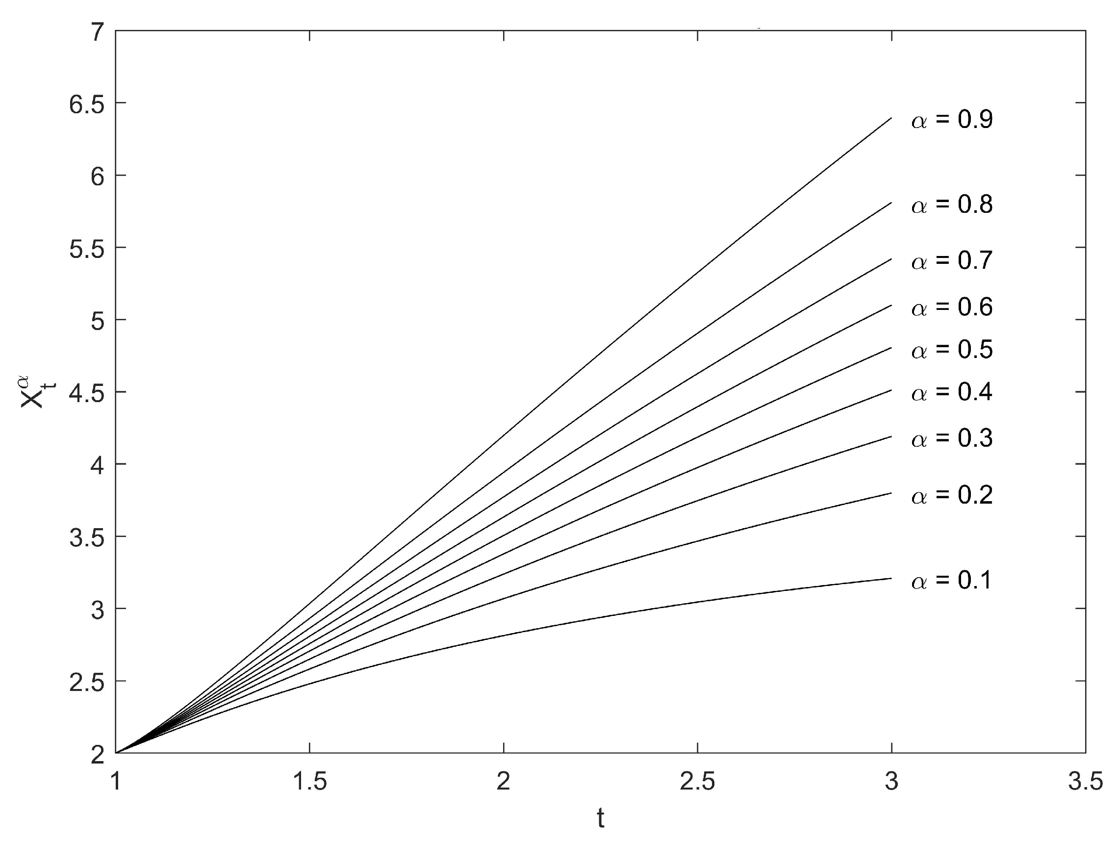
We choose the parameters as $p=1.5$ and $t=3$. Let the initial conditions be $x_0=2$, $x_1=1$ and the step length $h=0.01$, with $N=200$ and $\mathsf{\Delta }\alpha =0.01$. For different $\alpha$’s, the distribution of $X_t^{\alpha }$ is shown in Figure 3. The uncertainty distribution of $X_t$ at time $t=3$ for different orders p is shown in Figure 4.

Figure 3. Plots of $\alpha$-paths of (45) with order $p=1.5$.

Figure 4. The uncertainty distribution of $X_3$ with different orders p.

Let $J\left(x\right)=x^2$, $\epsilon =0.00001$, and $t=3$. For different orders p, the expected value of $J\left(X_t\right)$ can be computed by Algorithm 2, as shown in Table 8. As can be seen from Table 8, the larger the parameter p, the smaller the expected values of $J\left(X_t\right)$. Thus, when the analytic solution of the Caputo–Hadamard UFDE does not exist, we can obtain the numerical solution by the proposed Algorithm 1. The expected values of $J\left(X_t\right)$ can also be obtained by the proposed Algorithm 2.

Table 8. Expected values of $J\left(X_t\right)$ with different orders p.

p	$1.1$	$1.2$	$1.3$	$1.4$	$1.5$	$1.6$	$1.7$	$1.8$	$1.9$
$E\left[{X_3}^2\right]$	31.24	29.53	27.87	26.28	24.79	23.39	22.08	20.88	19.76

7. Conclusions

In this paper, we mainly discussed numerical algorithms for solving Caputo–Hadamard UFDEs. The definition of the $\alpha$-path was given, and the Caputo–Hadamard UFDE was connected with the Caputo–Hadamard FDE through the definition of the $\alpha$-path. An important theorem that the $\alpha$-path of a Caputo–Hadamard UFDE is the inverse uncertainty distribution of the solution was proved. For Caputo–Hadamard UFDEs driven by an independent Liu process, the theorem for calculating the expected value of a strictly monotonic function was proposed. Subsequently, a numerical algorithm was designed to calculate the inverse uncertainty distribution of solutions of Caputo–Hadamard UFDEs. At the same time, on the basis of Algorithm 1, an algorithm for solving the expected value of a strictly monotonic function was given by applying Simpson’s rule. Finally, some numerical examples were given to illustrate the accuracy and effectiveness of the proposed algorithm. For future work, we will discuss the stability of Hadamard UFDEs.