Fractal Perturbation of the Nadaraya–Watson Estimator

Abstract

One of the main tasks in the problems of machine learning and curve fitting is to develop suitable models for given data sets. It requires to generate a function to approximate the data arising from some unknown function. The class of kernel regression estimators is one of main types of nonparametric curve estimations. On the other hand, fractal theory provides new technologies for making complicated irregular curves in many practical problems. In this paper, we are going to investigate fractal curve-fitting problems with the help of kernel regression estimators. For a given data set that arises from an unknown function m, one of the well-known kernel regression estimators, the Nadaraya–Watson estimator $\widehat{m}$, is applied. We consider the case that m is Hölder-continuous of exponent $\beta$ with $0<\beta \le 1$, and the graph of m is irregular. An estimation for the expectation of $|\widehat{m}{-m|}^2$ is established. Then a fractal perturbation $f_{\left[\widehat{m}\right]}$ corresponding to $\widehat{m}$ is constructed to fit the given data. The expectations of $|f_{\left[\widehat{m}\right]}-\widehat{m}{|}^2$ and $|f_{\left[\widehat{m}\right]}{-m|}^2$ are also estimated.

1. Introduction

One of the main tasks in the problems of machine learning, curve fitting, signal analysis, and many statistical applications is to develop suitable models for given data sets. In many real-world applications, it requires to generate a function to interpolate or to approximate the data arising from some unknown function. In data-fitting problems, interpolation is usually applied when the data are noise-free, and regression is considered if we have noisy observations.

The theory of nonparametric modeling of a regression has been developed by many researchers. Several types of estimators and their statistical properties have been studied in the literature. The class of kernel estimators is one of the main types of nonparametric curve estimations, and the Nadaraya–Watson estimator, the Priestley–Chao estimator, and the Gasser–Müller estimator are widely used in applications. See [1,2,3,4,5,6] and references given in these books. In [7,8], the authors investigated the differences between several types of kernel regression estimators, and there is no answer to which of these estimators is the best since each of them has advantages and disadvantages.

Fractal theory provides another technology for making complicated curves and fitting experimental data. A fractal interpolation function (FIF) is a continuous function interpolating a given set of points, and the graph of a FIF is the attractor of an iterated function system. The concept of FIFs was introduced by Barnsley ([9,10]), and it has been developed to be the basis of an approximation theory for nondifferentiable functions. FIFs can also be applied to model discrete sequences ([11,12,13]). Various types of FIFs and their approximation properties were discussed in [14,15,16,17,18,19,20,21,22,23,24,25,26,27,28,29,30,31,32,33,34,35,36,37,38,39,40,41,42,43,44], and the references given in the literature. See also the book [45] for recent developments. In [46,47,48,49,50], the construction of FIFs for random data sets is given, and some statistical properties of such FIFs were investigated. In [51], the authors made a topological–geometric contribution for the development and applications of fractal models, which present periodic changes.

For a given data set that arises from an unknown function m, the purpose of this paper is not to establish a fractal function that interpolates points in the data set, but we aim to find a fractal function that has good approximation for these data points. In [52], the authors trained SVM by the chosen training data and then applied the SVM model to calculate the interpolation points used to construct a linear FIF. In this paper, we consider the Nadaraya–Watson estimator $\widehat{m}$ for some sample data chosen from a given data set, and establish an estimation for the expectation of $|\widehat{m}{-m|}^2$. Then a FIF $f_{\left[\widehat{m}\right]}$ corresponding to $\widehat{m}$ is constructed to fit the given data set, and the expectations of $|f_{\left[\widehat{m}\right]}-\widehat{m}{|}^2$ and $|f_{\left[\widehat{m}\right]}{-m|}^2$ are also estimated.

Throughout this paper, let $\mathcal{D}=\{(t_i,y_i)\in \mathbb{R}\times \mathbb{R}:i=0,1,\cdots ,N\}$ be a given data set, where N is an integer greater than or equal to 2, and $t_0<t_1<\cdots <t_N$. We take $t_0=0$ and $t_N=1$ for convenience. Let $I=[0,1]$ and $I_i=[t_{i-1},t_i]$ for $i=1,\cdots ,N$. Let $C\left[I\right]$ denote the set of all real-valued continuous functions defined on I. The set of functions in $C\left[I\right]$ that interpolate all points in $\mathcal{D}$ is denoted by $C_{\mathcal{D}}\left[I\right]$. Define ${\parallel f\parallel }_{\infty }={max}_{t\in I}\left|f\left(t\right)\right|$ for $f\in C\left[I\right]$. It is known that $(C\left[I\right],\parallel ·{\parallel }_{\infty })$ is a Banach space, and $C_{\mathcal{D}}\left[I\right]$ is a complete metric space, where the metric is induced by ${\parallel ·\parallel }_{\infty }$.

2. Construction of Fractal Interpolation Functions

In this section, we establish a fractal perturbation of a given function in $C\left[I\right]$. The construction given here has been treated in the literature (see [47]). We show the details here to make our paper more self-contained.

Let $u\in C\left[I\right]$ and $\mathcal{D}=\{(t_i,y_i):y_i=u\left(t_i\right),i=0,1,\cdots ,N\}$, where $0=t_0<t_1<\cdots <t_N=1$. Assume that the data points in $\mathcal{D}$ are non-collinear. For $i=1,\cdots ,N$, let $L_i:I\to I_i$ be a homeomorphism such that $L_i\left(0\right)=t_{i-1}$ and $L_i\left(1\right)=t_i$. Define $M_i:I\times \mathbb{R}\to \mathbb{R}$ by

$$M_i(t,y)=s_{i}y+u\left(L_i\left(t\right)\right)-s_{i}p\left(t\right),$$

(1)

where $-1<s_i<1$ and p is a continuous function on I such that $p\left(0\right)=u\left(0\right)$ and $p\left(1\right)=u\left(1\right)$. Then $M_i(0,u\left(0\right))=y_{i-1}$, $M_i(1,u\left(1\right))=y_i$, and

$$|M_i(t,y)-M_i(t,y^{*})|=|s_i\left|\right|y-y^{*}|\mathrm{for}\mathrm{all}t\in I\mathrm{and}y,y^{*}\in \mathbb{R}.$$

(2)

Define $W_i:I\times \mathbb{R}\to I_i\times \mathbb{R}$ by $W_i(t,y)=(L_i\left(t\right),M_i(t,y))$ for $i=1,\cdots ,N$. For $h\in C_{\mathcal{D}}\left[I\right]$, let $G_h=\{(t,h\left(t\right)):t\in I\}$. Then $W_i\left(G_h\right)=\{(L_i\left(t\right),M_i(t,h\left(t\right))):t\in I\}$. Since $L_i:I\to I_i$ is a homeomorphism, $W_i\left(G_h\right)$ can be written as

$$W_i\left(G_h\right)=\{(t,M_i(L_i^{-1}\left(t\right),h\left(L_i^{-1}\left(t\right)\right))):t\in I_i\}.$$

Hence $W_i\left(G_h\right)$ is the graph of the continuous function $h_i:I_i\to \mathbb{R}$ defined by $h_i\left(t\right)=M_i(L_i^{-1}\left(t\right),h\left(L_i^{-1}\left(t\right)\right))$. Define a mapping $T:C_{\mathcal{D}}\left[I\right]\to C_{\mathcal{D}}\left[I\right]$ by

$$T\left(h\right)\left(t\right)=h_i\left(t\right)=s_{i}h\left(L_i^{-1}\left(t\right)\right)+u\left(t\right)-s_{i}p\left(L_i^{-1}\left(t\right)\right),t\in I_i.$$

(3)

By $\left(3\right)$ we see that, for $g,h\in C_{\mathcal{D}}\left[I\right]$ and $t\in I_i$,

$$|T\left(g\right)\left(t\right)-T\left(h\right)\left(t\right)|\le |s_i\left|\right|g\left(L_i^{-1}\left(t\right)\right)-h\left(L_i^{-1}\left(t\right)\right)|.$$

Then

$${\parallel T\left(g\right)-T\left(h\right)\parallel }_{\infty }\le \underset{i=1,\cdots ,N}{max}|s_i|\left\{\underset{z\in I}{max}|g\left(z\right)-h\left(z\right)|\right\}\le s{\parallel g-h\parallel }_{\infty }.$$

Here $s=max\left\{\right|s_1|,\cdots ,|s_N\left|\right\}$. Since $0\le s<1$, we have the following theorem ([47], Theorem 2.1).

Theorem 1. 

The operator T given by $\left(3\right)$ is a contraction mapping on $C_{\mathcal{D}}\left[I\right]$.

Definition 1. 

The fixed point $f_{\left[u\right]}$ of T in $C_{\mathcal{D}}\left[I\right]$ is called a fractal interpolation function (FIF) on I corresponding to the continuous function u.

The FIF $f_{\left[u\right]}$ given in Definition 1 satisfies the following equation for $i=1,\cdots ,N$:

$$f_{\left[u\right]}\left(t\right)=s_i\left\{f_{\left[u\right]}\left(L_i^{-1}\left(t\right)\right)-p\left(L_i^{-1}\left(t\right)\right)\right\}+u\left(t\right),t\in I_i.$$

(4)

If $s_i=0$ for all i, then $f_{\left[u\right]}=u$. Therefore, $f_{\left[u\right]}$ can be treated as a fractal perturbation of u.

3. The Nadaraya–Watson Estimator

Let $\mathcal{D}=\{(t_i,y_i)\in \mathbb{R}\times \mathbb{R}:i=0,1,\cdots ,N\}$ be a given data set, where $0=t_0<t_1<\cdots <t_N=1$. Suppose that

$$Y_i=m\left(t_i\right)+{ϵ}_i,\mathrm{for}i=0,1,\cdots ,N,$$

(5)

where $m:[0,1]\to \mathbb{R}$ is an unknown function, and each $y_i$ is an observation of $Y_i$. Here, all ${ϵ}_i$ are independent stochastic disturbance terms with zero expectation, E$\left[{ϵ}_i\right]=0$, and finite variance, Var$\left[{ϵ}_i\right]\le {\sigma }^2<\infty$. In this section, we consider the Nadaraya–Watson estimator $\widehat{m}$ for $\mathcal{D}$ and establish an estimation for the expectation of $|\widehat{m}{-m|}^2$.

Consider the case that m is Hölder continuous of exponent $\beta$ with $0<\beta \le 1$, and the graph of m is irregular. Then, m satisfies the inequality with $0<\beta \le 1$ and $\lambda >0$:

$$|m\left(t\right)-m\left(t^{\prime }\right)|\le \lambda |t-t^{\prime }{|}^{\beta },t,t^{\prime }\in I.$$

(6)

The Nadaraya–Watson estimator $\widehat{m}$ of m is defined by

$$\widehat{m}\left(t\right)=\frac{{\sum }_{i=0}^N{k}_d(t-t_i)Y_i}{{\sum }_{j=0}^N{k}_d(t-t_j)},\mathrm{where}{k}_d\left(z\right)=\frac{1}{d}k\left(\frac{z}{d}\right).$$

(7)

Here $d>0$ is a bandwidth, and k is an integrable function defined on $\mathbb{R}$.

The function k is called a kernel and is usually assumed to be bounded and satisfies some integrable conditions. Some widely used kernels are given in ([2], p. 41) and ([5], p. 3), and the estimations using different kernels are usually numerically similar (see [6]). In this paper, we assume that there are positive numbers $C_1$, $C_2$, $\eta$, and R such that the kernel k satisfies the condition

$$C_1{\chi }_{[-\eta ,\eta ]}\left(z\right)\le k\left(z\right)\le C_2{\chi }_{[-R,R]}\left(z\right),z\in \mathbb{R}.$$

(8)

Condition (8) and its multidimensional form was considered in ([5], Theorem 1.7) and ([1], Theorem 5.1).

A new estimation for the bias of $\widehat{m}$ was obtained in [53]. Here, we give an estimation for E$\left[{(\widehat{m}\left(t\right)-m\left(t\right))}^2\right]$ in the following Theorem 2. Similar results were studied in [1,2,5], and other literature. The convergence rate of upper estimation obtained in Theorem 2 is the same as the known results.

The Nadaraya–Watson estimator $\widehat{m}$ given in (7) can be written in the form

$$\widehat{m}\left(t\right)=\sum _{i=0}^N{W}_i\left(t\right)Y_i,\mathrm{where}{W}_i\left(t\right)=\frac{k_d(t-t_i)}{{\sum }_{j=0}^N{k}_d(t-t_j)}.$$

(9)

Then ${\sum }_{i=0}^N{W}_i\left(t\right)=1$ for all t and

$$\mathbf{E}\left[\widehat{m}\left(t\right)\right]=\sum _{i=0}^N{W}_i\left(t\right)\mathbf{E}\left[Y_i\right]=\sum _{i=0}^N{W}_i\left(t\right)m\left(t_i\right).$$

(10)

In the following lemma, we give a lower bound for ${\sum }_{j=0}^N{k}_d(t-t_j)$. Define

$$a_N=\underset{1\le k\le N}{min}{t}_k-t_{k-1},A_N=\underset{1\le k\le N}{max}{t}_k-t_{k-1}.$$

(11)

Lemma 1. 

Let $0=t_0<t_1<\cdots <t_N=1$. Suppose that $k:\mathbb{R}\to \mathbb{R}$ and there are positive numbers $C_1$ and η such that $C_1{\chi }_{[-\eta ,\eta ]}\left(z\right)\le k\left(z\right)$ for $z\in \mathbb{R}$. Let $d>0$ and let $A_N$ and $k_d$ be defined in (11) and (7), respectively. Assume that $A_N<2d\eta$ and $A_N\le \frac{\alpha }{N}$ for some $\alpha >0$. Then for $0\le t\le 1$,

$$\sum _{j=0}^N{k}_d(t-t_j)\ge \frac{C_1\eta N}{\alpha }.$$

(12)

Proof. 

For $0\le t\le 1$, the condition $C_1{\chi }_{[-\eta ,\eta ]}\left(z\right)\le k\left(z\right)$ implies that

$$\sum _{j=0}^N{k}_d(t-t_j)=\frac{1}{d}\sum _{j=0}^{N}k\left(\frac{t-t_j}{d}\right)\ge \frac{C_1}{d}\sum _{j=0}^N{\chi }_{[-\eta ,\eta ]}\left(\frac{t-t_j}{d}\right)=\frac{C_1}{d}\left|E_{\eta }\left(t\right)\right|,$$

where $E_{\eta }\left(t\right)=\{t_j:j=0,1,\cdots ,N,\mathrm{and}|\frac{t-t_j}{d}|\le \eta \}$ and $|E_{\eta }\left(t\right)|$ is the number of elements of $E_{\eta }\left(t\right)$. Since $|\frac{t-t_j}{d}|\le \eta$ if and only if $t_j\in [t-d\eta ,t+d\eta ]\cap [0,1]$, we have $E_{\eta }\left(t\right)=\{t_j:j=0,1,\cdots ,N,\mathrm{and}{t}_j\in [t-d\eta ,t+d\eta ]\cap [0,1]$}.

For $t\in [d\eta ,1-d\eta ]$, we have $[t-d\eta ,t+d\eta ]\subseteq [0,1]$, and by the condition $A_N<2d\eta$, we see that $|E_{\eta }\left(t\right)|\ge \left[\frac{2d\eta }{A_N}\right]\ge 1$ and this implies $|E_{\eta }\left(t\right)|\ge \frac{d\eta }{A_N}$. For $t\in [0,d\eta )$, we have $[t-d\eta ,t+d\eta ]\cap [0,1]=[0,t+d\eta ]$ and $t_0=0\in E_{\eta }\left(t\right)$. Hence $|E_{\eta }\left(t\right)|\ge \left[\frac{t+d\eta }{A_N}\right]+1\ge 1$ and $|E_{\eta }\left(t\right)|\ge \frac{d\eta }{A_N}$. For $t\in (1-d\eta ,1]$, we have $[t-d\eta ,t+d\eta ]\cap [0,1]=[t-d\eta ,1]$ and $t_N=1\in E_{\eta }\left(t\right)$. Hence $|E_{\eta }\left(t\right)|\ge \left[\frac{1-t+d\eta }{A_N}\right]+1\ge 1$ and $|E_{\eta }\left(t\right)|\ge \frac{d\eta }{A_N}$. Then the condition $A_N\le \frac{\alpha }{N}$ implies $\left(12\right)$. □

Theorem 2. 

Let $\mathcal{D}$ be a given data set and assume that m satisfies $\left(6\right)$. Suppose that k satisfies $\left(8\right)$ and $\widehat{m}$ is defined by $\left(7\right)$. Assume that $A_N<2d\eta$ and $A_N\le \frac{\alpha }{N}$ for some $\alpha >0$. Then we have

$$\mathbf{E}\left[{(\widehat{m}\left(t\right)-m\left(t\right))}^2\right]\le {\lambda }^2{R}^{2\beta }{d}^{2\beta }+\left(\frac{\alpha C_2{\sigma }^2}{C_1\eta }\right)\frac{1}{Nd}.$$

(13)

Proof. 

We see that

$$\mathbf{E}\left[{(\widehat{m}\left(t\right)-m\left(t\right))}^2\right]={\{\mathbf{E}\left[\widehat{m}\left(t\right)\right]-m\left(t\right)\}}^2+\mathbf{E}\left[\widehat{m}{\left(t\right)}^2\right]-{\left(\mathbf{E}\left[\widehat{m}\left(t\right)\right]\right)}^2.$$

(14)

By (6) and (9)–(10), we have

$$|\mathbf{E}\left[\widehat{m}\left(t\right)\right]-m\left(t\right)|=\left|\sum _{i=0}^N{W}_i\left(t\right)(m\left(t_i\right)-m\left(t\right))\right|\le \lambda \sum _{i=0}^N{W}_i\left(t\right){|t_i-t|}^{\beta }.$$

Condition $\left(8\right)$ implies that $k\left(\frac{t-t_i}{d}\right)=0$ if $|\frac{t-t_i}{d}|>R$. Therefore,

$$|\mathbf{E}\left[\widehat{m}\left(t\right)\right]-m\left(t\right)|\le \lambda d^{\beta }\frac{{\sum }_{i=0}^{N}k\left(\frac{t-t_i}{d}\right){\left|\frac{t-t_i}{d}\right|}^{\beta }}{{\sum }_{j=0}^{N}k\left(\frac{t-t_j}{d}\right)}\le \lambda R^{\beta }{d}^{\beta }.$$

(15)

On the other hand, by $\left(8\right)$ and $\left(12\right)$, we also have

$$\underset{i,t}{sup}{W}_i\left(t\right)=\underset{i,t}{sup}\frac{k\left(\frac{t-t_i}{d}\right)}{{\sum }_{j=0}^{N}k\left(\frac{t-t_j}{d}\right)}\le \frac{\alpha C_2}{C_1\eta Nd}.$$

(16)

By (9), (10) and (5), we have

$$\mathbf{E}\left[\widehat{m}{\left(t\right)}^2\right]-{\left(\mathbf{E}\left[\widehat{m}\left(t\right)\right]\right)}^2=\mathbf{E}\left[{(\widehat{m}\left(t\right)-\mathbf{E}\left[\widehat{m}\left(t\right)\right])}^2\right]=\mathbf{E}\left[{\left(\sum _{i=0}^N{W}_i\left(t\right){ϵ}_i\right)}^2\right].$$

Since all ${ϵ}_i$ are independent and satisfy $\mathbf{E}\left[{ϵ}_i\right]=0$ and $\mathbf{Var}\left[{ϵ}_i\right]\le {\sigma }^2<\infty$, the condition ${\sum }_{i=0}^N{W}_i\left(t\right)=1$ and estimation $\left(16\right)$ imply that

$$\mathbf{E}\left[\widehat{m}{\left(t\right)}^2\right]-{\left(\mathbf{E}\left[\widehat{m}\left(t\right)\right]\right)}^2=\sum _{i=0}^N{W}_i{\left(t\right)}^2\mathbf{E}\left[{ϵ}_i^2\right]\le {\sigma }^2\left(\underset{i,t}{sup}{W}_i\left(t\right)\right)\sum _{i=0}^N{W}_i\left(t\right)\le \left(\frac{\alpha C_2{\sigma }^2}{C_1\eta }\right)\frac{1}{Nd}.$$

Then by (14) and (15), we have (13). □

For a given kernel k which satisfies $\left(8\right)$, estimation $\left(13\right)$ shows that $C_1$ and $\eta$ should be chosen so that $C_1\eta$ is as large as possible. The minimizer $d^{*}$ with respect to d of the right-hand side of $\left(13\right)$ can be obtained by setting $E\left(d\right)={\lambda }^2{R}^{2\beta }{d}^{2\beta }+\left(\frac{\alpha C_2{\sigma }^2}{C_1\eta N}\right)d^{-1}$, and then solve the equation

$$E^{\prime }\left(d\right)=\left(2\beta \right){\lambda }^2{R}^{2\beta }{d}^{2\beta -1}-\left(\frac{\alpha C_2{\sigma }^2}{C_1\eta N}\right)d^{-2}=0.$$

We have

$$d^{*}={\left(\frac{\alpha C_2{\sigma }^2}{2\beta C_1\eta {\lambda }^2{R}^{2\beta }}\right)}^{\frac{1}{2\beta +1}}{N}^{\frac{-1}{2\beta +1}}$$

(17)

and the upper estimate given in $\left(13\right)$ can be reduced to $C^{*}{N}^{-2\beta /(2\beta +1)}$, where $C^{*}$ depends on $\alpha$, $\beta$, $\lambda$, ${\sigma }^2$, $\eta$, R, $C_1$, and $C_2$.

4. Fractal Perturbation of the Nadaraya–Watson Estimator

In this section, we consider FIFs $f_{\left[\widehat{m}\right]}$ corresponding to the function $\widehat{m}$ and we establish estimations for the expectation of $|f_{\left[\widehat{m}\right]}-\widehat{m}{|}^2$ and $|f_{\left[\widehat{m}\right]}{-m|}^2$. Suppose that k is continuous and we replace each $Y_i$ in $\left(7\right)$ by $y_i$. Then $\widehat{m}\in C\left[I\right]$. By the construction given in Section 2 with $u=\widehat{m}$, we have a FIF $f_{\left[\widehat{m}\right]}$ on I that satisfies the equation for $i=1,\cdots ,N$:

$$f_{\left[\widehat{m}\right]}\left(t\right)=s_i\left\{f_{\left[\widehat{m}\right]}\left(L_i^{-1}\left(t\right)\right)-p\left(L_i^{-1}\left(t\right)\right)\right\}+\widehat{m}\left(t\right),t\in I_i.$$

(18)

Here, p is chosen to be the linear polynomial such that $p\left(0\right)=\widehat{m}\left(0\right)$ and $p\left(1\right)=\widehat{m}\left(1\right)$. Then we replace $y_i$ by $Y_i$ for each i and consider $f_{\left[\widehat{m}\right]}\left(t\right)$ a random variable for every $t\in I$. We are interested in estimations for $\parallel \mathrm{E}\left[\right|f_{\left[\widehat{m}\right]}{-m|}^2{]\parallel }_{\infty }$.

Theorem 3. 

Suppose that k is continuous and k satisfies $\left(8\right)$ with $R=1$ and $C_2=1$. Suppose that m satisfies $\left(6\right)$ and $\widehat{m}$ is defined by $\left(7\right)$. Let $M=max\left\{\right|m\left(t_i\right)|:i=0,1,\cdots ,N\}$. Assume that $A_N<2d\eta$, $A_N\le \frac{\alpha }{N}$, and $a_N\ge \frac{\tau }{N}$ for some $\alpha >0$ and $\tau >0$, where $A_N$ and $a_N$ are defined in $\left(11\right)$. Suppose that $0<s=max\left\{\right|s_1|,\cdots ,|s_N\left|\right\}<2^{-1/2}$ and $\parallel \mathbf{E}\left[\right|f_{\left[\widehat{m}\right]}-\widehat{m}{|}^2{]\parallel }_{\infty }<\infty$. Then we have

$$\begin{array}{cc}\hfill \parallel \mathrm{E}\left[\right|f_{\left[\widehat{m}\right]}-\widehat{m}{|}^2{]\parallel }_{\infty }& \le \left(\frac{72s^2{\alpha }^2(M^2+{\sigma }^2)}{(1-2s^2)C_1^2{\eta }^2{\tau }^2}\right)\frac{{(Nd+\tau )}^2}{{\left(Nd\right)}^2},\hfill \end{array}$$

(19)

$$\begin{array}{cc}\hfill \parallel \mathrm{E}\left[\right|f_{\left[\widehat{m}\right]}{-m|}^2{]\parallel }_{\infty }& \le \left(\frac{144s^2{\alpha }^2(M^2+{\sigma }^2)}{(1-2s^2)C_1^2{\eta }^2{\tau }^2}\right)\frac{{(Nd+\tau )}^2}{{\left(Nd\right)}^2}+2{\lambda }^2{d}^{2\beta }+\left(\frac{2\alpha {\sigma }^2}{C_1\eta }\right)\frac{1}{Nd}.\hfill \end{array}$$

(20)

Proof. 

For $t\in I_i$, $\left(18\right)$ implies

$$|f_{\left[\widehat{m}\right]}\left(t\right)-\widehat{m}{\left(t\right)|}^2\le 2s_i^2\left\{|f_{\left[\widehat{m}\right]}\left(L_i^{-1}\left(t\right)\right)-\widehat{m}\left(L_i^{-1}\left(t\right)\right){|}^2+{|\widehat{m}\left(L_i^{-1}\left(t\right)\right)-p\left(L_i^{-1}\left(t\right)\right)|}^2\right\},$$

and we have

$$\underset{t\in I_i}{sup}\mathrm{E}\left[\right|f_{\left[\widehat{m}\right]}\left(t\right)-\widehat{m}\left(t\right){|}^2]\le 2s_i^2\left(\underset{z\in I}{sup}\mathrm{E}\left[\right|f_{\left[\widehat{m}\right]}\left(z\right)-\widehat{m}{\left(z\right)|}^2]+\underset{z\in I}{sup}\mathbf{E}\left[\right|\widehat{m}\left(z\right)-p\left(z\right){|}^2]\right).$$

Then

$$\parallel \mathbf{E}\left[\right|f_{\left[\widehat{m}\right]}-\widehat{m}{|}^2{]\parallel }_{\infty }\le 2s^2\{\parallel \mathbf{E}[|f_{\left[\widehat{m}\right]}-\widehat{m}{|}^2{]\parallel }_{\infty }+\parallel \mathbf{E}\left[\right|\widehat{m}{-p|}^2{]\parallel }_{\infty }\}$$

and therefore

$$\parallel \mathbf{E}\left[\right|f_{\left[\widehat{m}\right]}-\widehat{m}{|}^2{]\parallel }_{\infty }\le \frac{2s^2}{1-2s^2}\parallel \mathbf{E}\left[\right|\widehat{m}{-p|}^2{]\parallel }_{\infty }.$$

(21)

Since p is the linear polynomial with $p\left(0\right)=\widehat{m}\left(0\right)$ and $p\left(1\right)=\widehat{m}\left(1\right)$, we have

$$p\left(t\right)=\widehat{m}\left(0\right)+(\widehat{m}\left(1\right)-\widehat{m}\left(0\right))t,t\in I,$$

(22)

and then

$$|\widehat{m}\left(t\right)-p\left(t\right)|=|(\widehat{m}\left(t\right)-\widehat{m}\left(0\right))(1-t)+(\widehat{m}\left(t\right)-\widehat{m}\left(1\right))t|.$$

The convexity of the square function $x\mapsto x^2$ implies that

$$|\widehat{m}{\left(t\right)-p\left(t\right)|}^2\le (1-t)|\widehat{m}\left(t\right)-\widehat{m}{\left(0\right)|}^2+t{|\widehat{m}\left(t\right)-\widehat{m}\left(1\right)|}^2$$

and therefore

$$\mathbf{E}\left[\right|\widehat{m}{\left(t\right)-p\left(t\right)|}^2]\le (1-t)\mathbf{E}[|\widehat{m}\left(t\right)-\widehat{m}{\left(0\right)|}^2]+t\mathbf{E}[|\widehat{m}\left(t\right)-\widehat{m}\left(1\right){|}^2],t\in I.$$

(23)

By $\left(9\right)$, $\widehat{m}\left(t\right)-\widehat{m}\left(1\right)={\sum }_{r=0}^N(W_r\left(t\right)-W_r\left(1\right))Y_r$. By $\left(8\right)$ with $R=1$, we see that if $t_r<1-d$, then $\frac{1-t_r}{d}>1$ and $k\left(\frac{1-t_r}{d}\right)=0$. This implies $W_r\left(1\right)=0$. For $t\in I$, if $t_r\notin [t-d,t+d]$, then $|\frac{t-t_r}{d}|>1$ and $k\left(\frac{t-t_r}{d}\right)=0$. This implies $W_r\left(t\right)=0$. Then

$$\widehat{m}\left(t\right)-\widehat{m}\left(1\right)=\sum _{r\in B_t}(W_r\left(t\right)-W_r\left(1\right))Y_r,$$

(24)

where $B_t=\{r:t_r\in [t-d,t+d]\mathrm{or}{t}_r\in [1-d,1]\}$. Let $\xi =\left[\frac{d}{a_N}\right]$. Then the number of elements in $B_t$ is less than $3(\xi +1)$.

By $\left(12\right)$ and $\left(8\right)$ with $C_2=1$, we have

$$|W_r\left(t\right)-W_r\left(1\right)|\le \frac{k_d(t-t_r)}{{\sum }_{j=0}^N{k}_d(t-t_j)}+\frac{k_d(1-t_r)}{{\sum }_{j=0}^N{k}_d(1-t_j)}\le \frac{2\alpha }{C_1\eta Nd}.$$

(25)

By $\left(5\right)$ we also have $\mathbf{E}\left[Y_r^2\right]=m{\left(t_r\right)}^2+{\sigma }^2$ for $r=0,1,\cdots ,N$. Condition $\left(6\right)$ shows that m is continuous and therefore m is bounded on I. Then for $t\in I$,

$$\begin{array}{cc}\hfill \mathbf{E}\left[\right|\widehat{m}\left(t\right)-\widehat{m}\left(1\right){|}^2]& \le \left\{\sum _{r\in B_t}{(W_r\left(t\right)-W_r\left(1\right))}^2\right\}\left\{\sum _{r\in B_t}\mathbf{E}\left[Y_r^2\right]\right\}\hfill \\ \hfill & \le {\left(\frac{2\alpha }{C_1\eta Nd}\right)}^2(M^2+{\sigma }^2){(3\xi +3)}^2.\hfill \end{array}$$

We also have the same estimate for $\mathbf{E}\left[\right|\widehat{m}\left(t\right)-\widehat{m}\left(0\right){|}^2]$.

By the condition $a_N\ge \frac{\tau }{N}$, we have $\xi \le \frac{d}{a_N}\le \frac{Nd}{\tau }$, and then $\left(23\right)$ can be reduced to

$$\mathbf{E}\left[\right|\widehat{m}\left(t\right)-p\left(t\right){|}^2]\le \left(\frac{36{\alpha }^2(M^2+{\sigma }^2)}{C_1^2{\eta }^2{\tau }^2}\right)\frac{{(Nd+\tau )}^2}{{\left(Nd\right)}^2},t\in I.$$

(26)

Thus, $\left(19\right)$ can be obtained by $\left(21\right)$ and $\left(26\right)$. Moreover, we have $\left(20\right)$ by $\left(13\right)$, $\left(19\right)$, and the inequality

$$\parallel \mathbf{E}\left[\right|f_{\left[\widehat{m}\right]}{-m|}^2{]\parallel }_{\infty }\le 2\parallel \mathbf{E}\left[\right|f_{\left[\widehat{m}\right]}-\widehat{m}{|}^2{]\parallel }_{\infty }+2\parallel \mathbf{E}\left[\right|\widehat{m}{-m|}^2{]\parallel }_{\infty }.$$

□

For a given kernel k, which satisfies condition $\left(8\right)$, estimation $\left(20\right)$ shows that $C_1$ and $\eta$ should be chosen so that $C_1\eta$ is as large as possible. If we choose $d=d^{*}$, where $d^{*}$ is given by $\left(17\right)$ with $C_2=1$ and $R=1$, then $\left(20\right)$ can be reduced to

$$\parallel \mathbf{E}\left[\right|f_{\left[\widehat{m}\right]}{-m|}^2{]\parallel }_{\infty }\le A{(1+D{N}^{\frac{-2\beta }{2\beta +1}})}^2+C^{*}{N}^{\frac{-2\beta }{2\beta +1}},$$

(27)

where $A=\frac{144s^2{\alpha }^2(M^2+{\sigma }^2)}{(1-2s^2)C_1^2{\eta }^2{\tau }^2}$ and D depends on $\lambda$, $\alpha$, $\beta$, $C_1$, $\eta$, $\tau$, ${\sigma }^2$, and $C^{*}$ depends on $\lambda$, $\alpha$, $\beta$, $C_1$, $\eta$, ${\sigma }^2$. Moreover, the constant M can be estimated by $\tilde{M}=max\left\{\right|y_0|,|y_1|,\cdots ,|y_N\left|\right\}$.

The right-hand side of $\left(27\right)$ tends to A when $N\to \infty$. In fact, if d is chosen so that $d\to 0$ and $Nd\to \infty$ as $N\to \infty$, then the right-hand side of $\left(20\right)$ tends to A as $N\to \infty$. Moreover, $A\to 0$ as $s\to 0$.

Example 1. 

The data set we used in this example is the Crude Oil WTI Futures daily highest price from 2021/7/19 to 2022/8/17. These data are opened and they can be obtained from the website https://www.investing.com/commodities/crude-oil-historical-data. There are 287 raw data and we chose 11 data as our sample subset $\mathcal{S}$. These data points are shown in Figure 1. We set $\mathcal{S}=\{(t_i,w_i):i=0,1,\cdots ,10\}$, where $t_i=\frac{i}{10}$ and $w_i$ are the Crude Oil WTI Futures daily highest prices in 2021/7/19, 8/26, 10/6, 11/16, 12/28, 2022/2/2, 3/9, 4/19, 5/30, 7/5, and 8/17.

Figure 1. Raw data and sample data.

Let $\widehat{m}$ be defined by $\left(7\right)$, with each $Y_i$ being replaced by $w_i$,

$$\widehat{m}\left(t\right)=\frac{{\sum }_{i=0}^{10}k\left(\frac{t-0.1\times i}{d}\right)w_i}{{\sum }_{j=0}^{10}k\left(\frac{t-0.1\times j}{d}\right)},$$

(28)

and choose k to be the Epanechnikov kernel $k\left(t\right)=0.75(1-t^2){\chi }_{\left\{\right|t|\le 1\}}$. Let $N=10$ and choose $R=1$, $C_2=1$, $\eta =\frac{1}{\sqrt{3}}$, $C_1=0.5$ in $\left(8\right)$. We estimate M by $max\{w_0,w_1,\cdots ,w_{10}\}$, and set $\alpha =1$ and $\tau =1$ in Theorem 3. Assume that $\beta =0.5$ in this example. The values of ${\sigma }^2$ and λ are estimated by the sample variance and $max\left\{\frac{|w_i-w_j|}{\sqrt{|t_i-t_j|}}:i,j=0,1,\cdots ,10,i\ne j\right\}$, respectively. By $\left(17\right)$, we set $d=0.092$.

We construct a FIF $f_{\left[\widehat{m}\right]}$ by the method given in Section 2 with linear functions $L_i$ and the linear polynomial p such that $L_i\left(0\right)=\frac{i-1}{10}$, $L_i\left(1\right)=\frac{i}{10}$, and $p\left(0\right)=\widehat{m}\left(0\right)$, $p\left(1\right)=\widehat{m}\left(1\right)$. The chosen values $s_1,\cdots ,s_{10}$ are given in Table 1.

Table 1. The values of $s_k$.

k	1	2	3	4	5	6	7	8	9	10
$s_k$	0.02	−0.03	0.08	−0.16	0.05	−0.26	−0.36	−0.06	−0.14	0.06

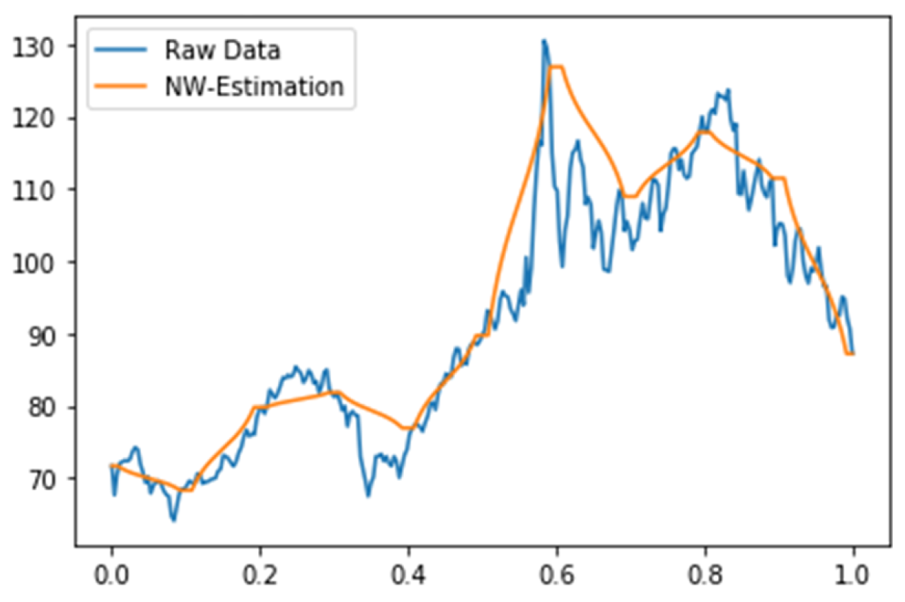
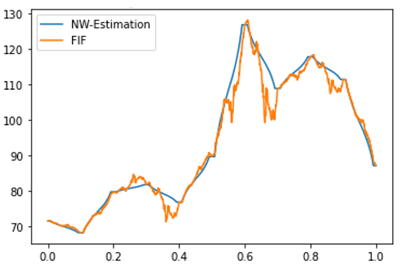
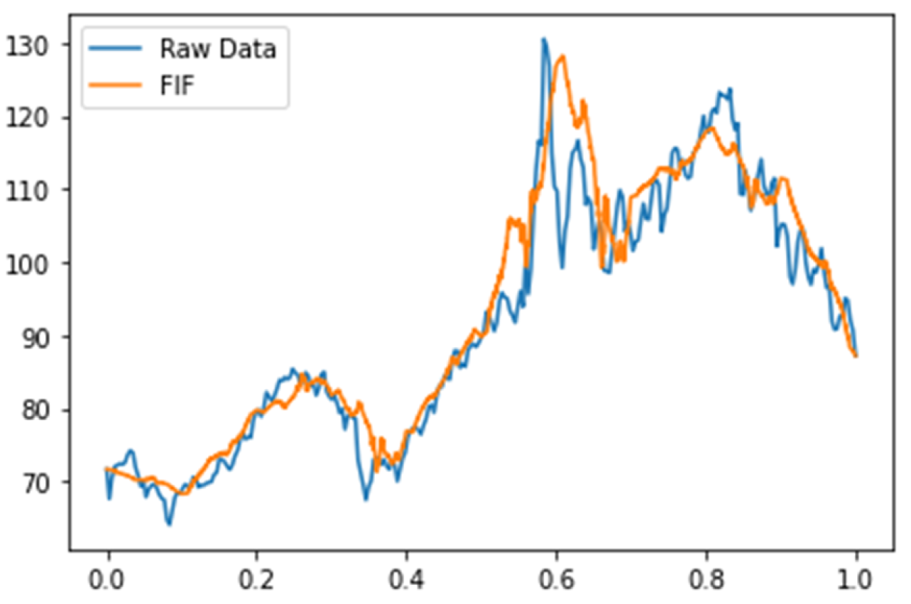
The graphs of raw data and $\widehat{m}$ are shown in Figure 2. The graphs of $\widehat{m}$ and $f_{\left[\widehat{m}\right]}$ are shown in Figure 3. The graphs of raw data and $f_{\left[\widehat{m}\right]}$ are shown in Figure 4.

Figure 2. Raw data and $\widehat{m}$.

Figure 3. $\widehat{m}$ and $f_{\left[\widehat{m}\right]}$.

Figure 4. Raw data and $f_{\left[\widehat{m}\right]}$.

5. Conclusions

The purpose of this paper is to construct a fractal interpolation function (FIF) that has good approximation for a given data set. We consider the Nadaraya–Watson estimator $\widehat{m}$ for some sample data chosen from a given data set, and then apply $\widehat{m}$ to construct a FIF $f_{\left[\widehat{m}\right]}$ to fit the given set of data points. The Nadaraya–Watson estimator is widely used in data-fitting problems, and its fractal perturbation is considered in our paper. The expectations of mean squared errors of such approximation are also estimated. By the figures given in Example 1, we may see the quality of curve fitting by a FIF, which is constructed from $\widehat{m}$ with 11 sample points to fit the 287 raw data points. We see that the error of approximation can be decreased by choosing more sample data.

In this paper, we construct a FIF to fit a given data set with the help of the Nadaraya–Watson estimator. In fact, the Priestley–Chao estimator, the Gasser–Müller estimator, and other types of kernel regression estimators can also be used in our approach. Nonparametric regression has been studied for a long time. Several types of models with their theoretical results and applications are widely developed by many researchers. Fractal perturbations of these models are worth investigating in the field of fractal curve fitting.

References

- Györfi, L.; Kohler, M.; Krzyzak, A.; Walk, H. A Distribution-Free Theory of Nonparametric Regression; Springer: New York, NY, USA, 2002. [Google Scholar]
- Härdle, W.; Müller, M.; Sperlich, S.; Werwatz, A. Nonparametric and Semiparametric Models; Springer: New York, NY, USA, 2004. [Google Scholar]
- Hart, J.D. Nonparametric Smoothing and Lack-of-Fit Tests; Springer: New York, NY, USA, 1997. [Google Scholar]
- Li, Q.; Racine, J.S. Nonparametric Econometrics; Princeton University Press: Mercer County, NJ, USA, 2007. [Google Scholar]
- Tsybakov, A.B. Introduction to Nonparametric Estimation; Springer: New York, NY, USA, 2009. [Google Scholar]
- Wasserman, L. All of Nonparametric Statistics; Springer: New York, NY, USA, 2006. [Google Scholar]
- Chu, C.-K.; Marron, J.S. Choosing a kernel regression estimator. Stat. Sci. 1991, 6, 404–436. [Google Scholar] [CrossRef]
- Jones, M.C.; Davies, S.J.; Park, B.U. Versions of kernel-type regression estimators. J. Amer. Statist. Assoc. 1994, 89, 825–832. [Google Scholar] [CrossRef]
- Barnsley, M.F. Fractal functions and interpolation. Constr. Approx. 1986, 2, 303–329. [Google Scholar] [CrossRef]
- Barnsley, M.F. Fractals Everywhere; Academic Press: Orlando, FL, USA, 1988. [Google Scholar]
- Marvasti, M.A.; Strahle, W.C. Fractal geometry analysis of turbulent data. Signal Process. 1995, 41, 191–201. [Google Scholar] [CrossRef]
- Mazel, D.S. Representation of discrete sequences with three-dimensional iterated function systems. IEEE Trans. Signal Process. 1994, 42, 3269–3271. [Google Scholar] [CrossRef]
- Mazel, D.S.; Hayes, M.H. Using iterated function systems to model discrete sequences. IEEE Trans. Signal Process. 1992, 40, 1724–1734. [Google Scholar] [CrossRef]
- Balasubramani, N. Shape preserving rational cubic fractal interpolation function. J. Comput. Appl. Math. 2017, 319, 277–295. [Google Scholar] [CrossRef]
- Balasubramani, N.; Guru Prem Prasad, M.; Natesan, S. Shape preserving α-fractal rational cubic splines. Calcolo 2020, 57, 21. [Google Scholar] [CrossRef]
- Barnsley, M.F.; Elton, J.; Hardin, D.; Massopust, P. Hidden variable fractal interpolation functions. SIAM J. Math. Anal. 1989, 20, 1218–1242. [Google Scholar] [CrossRef]
- Barnsley, M.F.; Massopust, P.R. Bilinear fractal interpolation and box dimension. J. Approx. Theory 2015, 192, 362–378. [Google Scholar] [CrossRef]
- Chand, A.K.B.; Kapoor, G.P. Generalized cubic spline fractal interpolation functions. SIAM J. Numer. Anal. 2006, 44, 655–676. [Google Scholar] [CrossRef]
- Chand, A.K.B.; Navascués, M.A. Natural bicubic spline fractal interpolation. Nonlinear Anal. 2008, 69, 3679–3691. [Google Scholar] [CrossRef]
- Chand, A.K.B.; Navascués, M.A. Generalized Hermite fractal interpolation. Rev. Real Acad. Cienc. Zaragoza 2009, 64, 107–120. [Google Scholar]
- Chand, A.K.B.; Tyada, K.R. Constrained shape preserving rational cubic fractal interpolation functions. Rocky Mt. J. Math. 2018, 48, 75–105. [Google Scholar] [CrossRef]
- Chand, A.K.B.; Vijender, N.; Viswanathan, P.; Tetenov, A.V. Affine zipper fractal interpolation functions. BIT Numer. Math. 2020, 60, 319–344. [Google Scholar] [CrossRef]
- Chand, A.K.B.; Viswanathan, P. A constructive approach to cubic Hermite fractal interpolation function and its constrained aspects. BIT Numer. Math. 2013, 53, 841–865. [Google Scholar] [CrossRef]
- Chandra, S.; Abbas, S.; Verma, S. Bernstein super fractal interpolation function for countable data systems. Numer. Algorithms 2022. [Google Scholar] [CrossRef]
- Dai, Z.; Wang, H.-Y. Construction of a class of weighted bivariate fractal interpolation functions. Fractals 2022, 30, 2250034. [Google Scholar] [CrossRef]
- Katiyar, S.K.; Chand, A.K.B. Shape preserving rational quartic fractal functions. Fractals 2019, 27, 1950141. [Google Scholar] [CrossRef]
- Katiyar, S.K.; Chand, A.K.B.; Kumar, G.S. A new class of rational cubic spline fractal interpolation function and its constrained aspects. Appl. Math. Comput. 2019, 346, 319–335. [Google Scholar] [CrossRef]
- Luor, D.-C. Fractal interpolation functions with partial self similarity. J. Math. Anal. Appl. 2018, 464, 911–923. [Google Scholar] [CrossRef]
- Massopust, P.R. Fractal Functions, Fractal Surfaces, and Wavelets; Academic Press: San Diego, CA, USA, 1994. [Google Scholar]
- Massopust, P.R. Interpolation and Approximation with Splines and Fractals; Oxford University Press: New York, NY, USA, 2010. [Google Scholar]
- Miculescu, R.; Mihail, A.; Pacurar, C.M. A fractal interpolation scheme for a possible sizeable set of data. J. Fractal Geom. 2022. [Google Scholar] [CrossRef]
- Navascués, M.A. Fractal approximation. Complex Anal. Oper. Theory 2010, 4, 953–974. [Google Scholar] [CrossRef]
- Navascués, M.A. Fractal bases of Lp spaces. Fractals 2012, 20, 141–148. [Google Scholar] [CrossRef]
- Navascués, M.A.; Chand, A.K.B. Fundamental sets of fractal functions. Acta Appl. Math. 2008, 100, 247–261. [Google Scholar] [CrossRef]
- Navascués, M.A.; Pacurar, C.; Drakopoulos, V. Scale-free fractal interpolation. Fractal Fract. 2022, 6, 602. [Google Scholar] [CrossRef]
- Prasad, S.A. Super coalescence hidden-variable fractal interpolation functions. Fractals 2021, 29, 2150051. [Google Scholar] [CrossRef]
- Ri, S.; Drakopoulos, V. Generalized fractal interpolation curved lines and surfaces. Nonlinear Stud. 2021, 28, 427–488. [Google Scholar]
- Tyada, K.R.; Chand, A.K.B.; Sajid, M. Shape preserving rational cubic trigonometric fractal interpolation functions. Math. Comput. Simul. 2021, 190, 866–891. [Google Scholar] [CrossRef]
- Vijender, N. Fractal perturbation of shaped functions: Convergence independent of scaling. Mediterr. J. Math. 2018, 15, 211. [Google Scholar] [CrossRef]
- Viswanathan, P. A revisit to smoothness preserving fractal perturbation of a bivariate function: Self-Referential counterpart to bicubic splines. Chaos Solitons Fractals 2022, 157, 111885. [Google Scholar] [CrossRef]
- Viswanathan, P.; Chand, A.K.B. Fractal rational functions and their approximation properties. J. Approx. Theory 2014, 185, 31–50. [Google Scholar] [CrossRef]
- Viswanathan, P.; Chand, A.K.B. α-fractal rational splines for constrained interpolation. Electron. Trans. Numer. Anal. 2014, 41, 420–442. [Google Scholar]
- Viswanathan, P.; Navascués, M.A.; Chand, A.K.B. Associate fractal functions in Lp-spaces and in one-sided uniform approximation. J. Math. Anal. Appl. 2016, 433, 862–876. [Google Scholar] [CrossRef]
- Wang, H.-Y.; Yu, J.-S. Fractal interpolation functions with variable parameters and their analytical properties. J. Approx. Theory 2013, 175, 1–18. [Google Scholar] [CrossRef]
- Banerjee, S.; Gowrisankar, A. Frontiers of Fractal Analysis Recent Advances and Challenges; CRC Press: Boca Raton, FL, USA, 2022. [Google Scholar]
- Kumar, M.; Upadhye, N.S.; Chand, A.K.B. Linear fractal interpolation function for data set with random noise. Fractals, 2022; accepted. [Google Scholar] [CrossRef]
- Luor, D.-C. Fractal interpolation functions for random data sets. Chaos Solitons Fractals 2018, 114, 256–263. [Google Scholar] [CrossRef]
- Luor, D.-C. Statistical properties of linear fractal interpolation functions for random data sets. Fractals 2018, 26, 1850009. [Google Scholar] [CrossRef]
- Luor, D.-C. Autocovariance and increments of deviation of fractal interpolation functions for random datasets. Fractals 2018, 26, 1850075. [Google Scholar] [CrossRef]
- Luor, D.-C. On the distributions of fractal functions that interpolate data points with Gaussian noise. Chaos Solitons Fractals 2020, 135, 109743. [Google Scholar] [CrossRef]
- Caldarola, F.; Maiolo, M. On the topological convergence of multi-rule sequences of sets and fractal patterns. Soft Comput. 2020, 24, 17737–17749. [Google Scholar] [CrossRef]
- Wang, H.-Y.; Li, H.; Shen, J.-Y. A novel hybrid fractal interpolation-SVM model for forecasting stock price indexes. Fractals 2019, 27, 1950055. [Google Scholar] [CrossRef]
- Tosatto, S.; Akrour, R.; Peters, J. An upper bound of the bias of Nadaraya-Watson kernel regression under Lipschitz assumptions. Stats 2021, 4, 1–17. [Google Scholar] [CrossRef]
Publisher’s Note: MDPI stays neutral with regard to jurisdictional claims in published maps and institutional affiliations. |
© 2022 by the authors. Licensee MDPI, Basel, Switzerland. This article is an open access article distributed under the terms and conditions of the Creative Commons Attribution (CC BY) license (https://creativecommons.org/licenses/by/4.0/).