Multiscale Approach for Bounded Deformation Image Registration

Abstract

Deformable image registration is a very important topic in the field of image processing. It is widely used in image fusion and shape analysis. Generally speaking, image registration models can be divided into two categories: smooth registration and non-smooth registration. During the last decades, many smooth registration models (i.e., diffeomorphic registration) were proposed. However, image with strong noise may lead to discontinuous deformation, which cannot be modelled by smooth registration. To simulate this kind of deformation, some non-smooth registration models were also proposed. However, numerical algorithms for these models are easily trapped into a local minimum because of the nonconvexity of the object functional. To overcome the local minimum of the object functional, we propose a multiscale approach for a non-smooth registration model: the bounded deformation (BD) model. The convergence of the approach is shown, and numerical tests are also performed to show the good performance of the proposed multiscale approach.

1. Introduction

Image registration refers to the matching of coordinates of different images, which are obtained in different time periods or by different imaging techniques. As one of the most challenging tasks in image processing, image registration has been widely used in remote sensing data analysis, computer vision, medical imaging, and other fields [1,2,3,4,5,6,7,8]. Many image registration models have been proposed during recent decades, for example, the Demons model [9], vectorial total variation model (VTV model) [10], and fractional-order model [11]. For more details, one can refer to [12]. Mathematically, image registration is stated in the following way. Suppose that $\mathsf{\Omega }\subset {\mathbb{R}}^2$ is an open bounded set and $T,D:\mathsf{\Omega }\to \mathbb{R}$ are two real functions defined on $\mathsf{\Omega }$. In image registration, T and D are viewed as two images, the source image and target image, respectively. The goal of registration is to find a geometric deformation $\mathbf{h}:\mathsf{\Omega }\to \mathsf{\Omega }$ such that the deformed image $T\circ \mathbf{h}(·)$ looks like $D(·)$ as much as possible. Concerning the problem of how to characterize the similarity between $T\circ \mathbf{h}(·)$ and $D(·)$, many metrics are proposed, such as the normalized cross correlation (NCC) [13,14], the normalized mutual information (NMI) [14], and the sum of squared distance (SSD) [15]. We mainly focus on mono-modality image registration. Therefore, SSD is used in this paper. That is, we aim to find the minimum of the SSD, which is defined by

$$\begin{array}{c}\hfill {\int }_{\mathsf{\Omega }}{[T\left(\mathbf{h}\left(\mathbf{x}\right)\right)-D\left(\mathbf{x}\right)]}^{2}d\mathbf{x}.\end{array}$$

(1)

where $\mathbf{x}=\left(x_1,x_2\right)$ and in small deformable image registration, $\mathbf{h}\left(\mathbf{x}\right)$ is approximately divided into trivial identity part $\mathbf{x}$ and displacement part $\mathbf{u}\left(\mathbf{x}\right)=\left(u_1\left(\mathbf{x}\right),u_2\left(\mathbf{x}\right)\right)$, i.e., $\mathbf{h}\left(\mathbf{x}\right)\triangleq \mathbf{x}+\mathbf{u}\left(\mathbf{x}\right)$. With these notations, the variational framework of image registration is formulated as:

$$\mathbf{u}=arg\underset{\mathbf{u}\in \mathcal{K}}{min}S\left(\mathbf{u}\right),$$

(2)

where, in here and in what follows, $S\left(\mathbf{u}\right)={\int }_{\mathsf{\Omega }}{[T(\mathbf{x}+\mathbf{u}\left(\mathbf{x}\right))-D\left(\mathbf{x}\right)]}^{2}d\mathbf{x}$, $\mathcal{K}$ is an admissible solution set.

Equation (2) is ill-posed [16,17]. A common way to overcome the ill-posedness is to add some regularization $R\left(\mathbf{u}\right)$ [11,12,13,15,16,17,18,19,20,21,22]. Based on this idea, the image registration model is reformulated as follows:

$$\mathbf{u}=arg\underset{\mathbf{u}\in \mathcal{K}}{min}S\left(\mathbf{u}\right)+\lambda R\left(\mathbf{u}\right),$$

(3)

where $\lambda >0$ is a constant to balance $R\left(\mathbf{u}\right)$ and $S\left(\mathbf{u}\right)$.

For different applications, different regularizations are introduced. For instance, in order to induce a diffusion type model, $R\left(\mathbf{u}\right)={∥▿\mathbf{u}∥}_{L^2\left(\mathsf{\Omega }\right)}^2$ is adopted in [23]. In addition, for the purpose of fitting the fractional-order smoothness of image texture, some fractional-order regularizations [24] are also introduced. For all these models, the diffeomorphic image registration models have become the focus of several groups [11,15,19,20,24,25,26,27,28,29]. In diffeomorphic registration, one is expected to produce a deformation $\mathbf{h}:\mathsf{\Omega }\to \mathsf{\Omega }$, which is a continuous bijection (1-to-1 and onto). By constraining the deformation into this kind of mapping, the topology of the object tissue is preserved. This is an advantage of diffeomorphic image registration. However, in some applications, i.e., the image pairs T and D with strong noises or pathological tissues, the registration deformation may be discontinuous. For example, in respiratory movement, the diaphragm is severely deformed but the chest remains almost rigid [30], which leads to discontinuous deformation. This discontinuous deformation cannot be well simulated by diffeomorphic image registration models. To simulate discontinuous deformation, some other image registration models were also proposed [11,24]. In [30], a registration model was introduced by letting $R\left(\mathbf{u}\right)={∥▿\mathbf{u}∥}_{L^1\left(\mathsf{\Omega }\right)}$. This is called total variation (TV) registration. As we all know, TV preserves the edge of tissue well. However, serious staircase effect occurs in the TV model. To overcome the staircase effect of the TV model, some image registration models were also proposed for improvement, for instance, the bounded deformation (BD) model [12]. In [12], by viewing the image process as an elastic deformation, the authors propose a bounded deformation model, which addresses the discontinuous deformation well. However, the algorithm in [12] is easily trapped into a local minimum of object functional $S\left(\mathbf{u}\right)+\lambda R\left(\mathbf{u}\right)$ because it is non-convex on $\mathbf{u}$. In fact, most of the published registration algorithms are all easily trapped into local minimum, which is caused by the non-convexity of the object functional. To overcome this problem, Han, Wang, and Zhang [25] proposed a multiscale image registration approach for 2D diffeomorphic image registration. Theoretical results and numerical tests are also presented in [25] to validate the fact that the multiscale approach can effectively overcome the local minimum of the object functional for image registration. Note that the multiscale approach in [25] is only suitable for diffeomorphic image registration. As an extension, we propose a multiscale approach for BD model, which can overcome the local minimum of the object functional and simulate the discontinuous deformation well. The proposed multiscale approach is essentially an iterative process. The convergence of the iterative process is shown, and several numerical tests are performed to show the good performance of the proposed multiscale approach.

The rest of the paper is organized as follows. In Section 2, we propose a multiscale image registration approach and show the convergence of the proposed approach. In Section 3, an image registration algorithm of the proposed multiscale approach is presented. In Section 4, several numerical tests are performed to show the good performance of the proposed multiscale approach.

2. Proposed Model

In [12], authors proposed a BD image registration model, which is formulated as follows:

$$\mathbf{u}=arg\underset{\mathbf{u}\in \mathcal{K}}{min}\mathsf{\Theta }S\left(\mathbf{u}\right)+\lambda R\left(\mathbf{u}\right),$$

(4)

where $\mathsf{\Theta },\lambda >0$, $R\left(\mathbf{u}\right)={\int }_{\mathsf{\Omega }}∥▿\mathbf{u}+{▿}^T\mathbf{u}∥d\mathbf{x}$, $\mathcal{K}=\left\{\mathbf{u}=(u_1,u_2)\in BD\left(\mathsf{\Omega }\right){\left|\mathbf{u}\right|}_{\partial \mathsf{\Omega }}=\mathbf{0}\right\}$, $\mathsf{\Omega }=$$(a_1,b_1)\times (a_1,b_1)$ and $BD\left(\mathsf{\Omega }\right)=\left\{\mathbf{u}\in L^1\left(\mathsf{\Omega };{\mathbb{R}}^2\right)|\left|\epsilon \left(\mathbf{u}\right)\right|\left(\mathsf{\Omega }\right)<\infty \right\}$, $\left|\epsilon \left(\mathbf{u}\right)\right|\left(\mathsf{\Omega }\right)=$${\int }_{\mathsf{\Omega }}∥▿\mathbf{u}+{▿}^T\mathbf{u}∥d\mathbf{x}$, there $L^1(\mathsf{\Omega };{\mathbb{R}}^2)=\left\{\mathbf{u}:\mathsf{\Omega }\to {\mathbb{R}}^2|{\int }_{\mathsf{\Omega }}\left|\mathbf{u}\left(\mathbf{x}\right)\right|d\mathbf{x}<\infty \right\}$. Here, the $L^1$ norm is defined as follows: ${∥▿\mathbf{u}∥}_1={\int }_{\mathsf{\Omega }}\left|▿\mathbf{u}\right|d\mathbf{x}={\int }_{\mathsf{\Omega }}\sqrt{{\sum }_{i=1}^2{\left|▿{\mathbf{u}}_i\right|}^2}d\mathbf{x}$.

The existence of the solution of (4) is proved in [12]. Moreover, an explicit scheme for (4) is also presented. However, the proposed algorithm in [12] is easily trapped into a local minimum of the object functional (4), because the object functional in (4) is non-convex on $\mathbf{u}$. To overcome the local minimum of the object functional, we extend the diffeomorphism-based multiscale approach in [25] into the BD model (4) by setting an increasing parameter sequence $\left\{{\mathsf{\Theta }}_n\right\}$ in each iteration. The proposed multiscale approach for BD model is listed as follows:

• Step 1: Solving the following variational problem to got an initial value:

  $${\mathbf{u}}^0=arg\underset{\mathbf{u}\in \mathcal{K}}{min}{\mathsf{\Theta }}_0{\int }_{\mathsf{\Omega }}{\left|T\circ \mathbf{h}\left(\mathbf{x}\right)-D\left(\mathbf{x}\right)\right|}^{2}d\mathbf{x}+\lambda R\left(\mathbf{u}\right),$$

  (5)

  where, $\mathbf{h}\left(\mathbf{x}\right)=\mathbf{x}+\mathbf{u}\left(\mathbf{x}\right)$ and ${\mathsf{\Theta }}_0>0$. Based on (5), we defined ${\widehat{\mathbf{h}}}_0\left(\mathbf{x}\right)=\mathbf{x}+{\mathbf{u}}^0\left(\mathbf{x}\right)$.
• Step 2: Based on the deformation ${\widehat{\mathbf{h}}}_0\left(\mathbf{x}\right)$ in Step 1, we updated the source image by $T\circ {\widehat{\mathbf{h}}}_0(·)$ and solved the following variational problem to get a new displacement filed ${\mathbf{u}}^1$:

  $${\mathbf{u}}^1=arg\underset{\mathbf{u}\in \mathcal{K}}{min}{\mathsf{\Theta }}_1{\int }_{\mathsf{\Omega }}{\left|T\circ {\widehat{\mathbf{h}}}_0(\mathbf{x}+\mathbf{u}\left(\mathbf{x}\right))-D\left(\mathbf{x}\right)\right|}^{2}d\mathbf{x}+\lambda R\left(\mathbf{u}\right),$$

  (6)

  where ${\mathsf{\Theta }}_1>0$. Based on the result of (6), we defined ${\mathbf{h}}_1\left(\mathbf{x}\right)=\mathbf{x}+{\mathbf{u}}^1\left(\mathbf{x}\right)$ and ${\widehat{\mathbf{h}}}_1\left(\mathbf{x}\right)={\widehat{\mathbf{h}}}_0\circ {\mathbf{h}}_1\left(\mathbf{x}\right)$.

  $$⋮$$
• Step n: We updated the source image by $T\circ {\widehat{\mathbf{h}}}_{n-1}(·)$ and solved the following variational problem:

  $$\begin{array}{c}\hfill {\mathbf{u}}^n=arg\underset{\mathbf{u}\in \mathcal{K}}{min}{\mathsf{\Theta }}_n{\int }_{\mathsf{\Omega }}{\left|T\circ {\widehat{\mathbf{h}}}_{n-1}(\mathbf{x}+\mathbf{u}\left(\mathbf{x}\right))-D\left(\mathbf{x}\right)\right|}^{2}d\mathbf{x}+\lambda R\left(\mathbf{u}\right),\end{array}$$

  (7)

  where ${\mathsf{\Theta }}_n>0$. Based on (7), we defined ${\mathbf{h}}_n\left(\mathbf{x}\right)=\mathbf{x}+{\mathbf{u}}^n\left(\mathbf{x}\right)$ and ${\widehat{\mathbf{h}}}_n\left(\mathbf{x}\right)={\widehat{\mathbf{h}}}_{n-1}\circ {\mathbf{h}}_n\left(\mathbf{x}\right)$. We repeated this process until it reached the desired accuracy.

Remark 1.

 (5)–(7) is a process of function composition, which we can write uniformly as follows:

$${\mathit{u}}^n=arg\underset{\mathit{u}\in \mathcal{K}}{min}{E}_n\left(\mathit{u}\right)\forall n\in \mathbb{N}.$$

(8)

where $T_n\left(\mathit{x}\right)=T\circ {\widehat{\mathit{h}}}_{n-1}\left(\mathit{x}\right)$, $E_n\left(\mathit{u}\right)=S_n\left(\mathit{u}\right)+\lambda R\left(\mathit{u}\right)$, $S_n\left(\mathit{u}\right)={\mathsf{\Theta }}_n{\int }_{\mathsf{\Omega }}{\left|T_n(\mathit{x}+\mathit{u}\left(\mathit{x}\right))-D\left(\mathit{x}\right)\right|}^{2}d\mathit{x}.$

Note that we set ${\mathsf{\Theta }}_n$ to be an increasing sequence in (8) for the following two reasons:

• It increases the ratio of the similarity term $S_n\left(\mathit{u}\right)$ in the object functional. Benefiting from this setting, $S_n\left(\mathit{u}\right)$ plays a dominant role in object functional as n is large enough. This improves the accuracy of image registration.
• An increasing ${\mathsf{\Theta }}_n$ helps the algorithm get out of the local minimum of the object functional in former iterative steps.

For the selection of ${\left\{{\mathsf{\Theta }}_n\right\}}_{n=1}^{K_M}$ in the actual calculation, we set it as an exponential function, i.e., ${\mathsf{\Theta }}_n=a^n\times {\mathsf{\Theta }}_0(n\in {\mathbb{N}}^{+})$, where $K_M$ is the maximum scale number. The registration result is optimized by adjusting the values of parameters a and ${\mathsf{\Theta }}_0$.

Theorem 1.

Define $\overline{\mathcal{K}}=\left\{\mathit{h}={\mathit{h}}_0\circ {\mathit{h}}_1\cdots \circ {\mathit{h}}_n\cdots \mid {\mathit{h}}_i\left(\mathit{x}\right)=\mathit{x}+{\mathit{u}}_i\left(\mathit{x}\right)and{\mathit{u}}_i\in \mathcal{K}\right\}$ and set $\left\{{\mathsf{\Theta }}_n\right\}$ to be an upper bounded sequence with ${\mathsf{\Theta }}_n\gg \lambda$ as n is large enough, then the deformation ${\widehat{\mathit{h}}}_n\left(·\right)$ induced by (5)–(7) converges to the global minimizer of $S\left(\mathit{u}\right)$ on $\overline{\mathcal{K}}$.

Proof. 

By the fact $\mathbf{0}\in \mathcal{K}$, we know that $E_n\left({\mathbf{u}}^n\right)\le E_n\left(\mathbf{0}\right)$ for any $n\in {\mathbb{N}}^{+}$.

That is,

$$\begin{array}{cc}\hfill E_n\left({\mathbf{u}}^n\right)& \hfill ={\mathsf{\Theta }}_n{∥T\circ {\widehat{\mathbf{h}}}_n(·)-D(·)∥}_{L^2\left(\mathsf{\Omega }\right)}^2+\lambda R\left({\mathbf{u}}^n\right)\hfill \\ & \hfill \le {\mathsf{\Theta }}_n{∥T\circ {\widehat{\mathbf{h}}}_{n-1}(·)-D(·)∥}_{L^2\left(\mathsf{\Omega }\right)}^2=E_n\left(\mathbf{0}\right).\hfill \end{array}$$

(9)

Therefore,

$$\begin{array}{c}\hfill {∥T\circ {\widehat{\mathbf{h}}}_n(·)-D(·)∥}_{L^2\left(\mathsf{\Omega }\right)}^2\le {∥T\circ {\widehat{\mathbf{h}}}_{n-1}(·)-D(·)∥}_{L^2\left(\mathsf{\Omega }\right)}^2\forall n\in {\mathbb{N}}^{+}.\end{array}$$

(10)

This implies, $\left\{{∥T\circ {\widehat{\mathbf{h}}}_n(·)-D(·)∥}_{L^2\left(\mathsf{\Omega }\right)}^2\right\}$ is a decreasing sequence with lower bound. By the monotone bounded convergence theorem [31], we know that the sequence $\left\{{∥T\circ {\widehat{\mathbf{h}}}_n(·)-D(·)∥}_{L^2\left(\mathsf{\Omega }\right)}^2\right\}$ is convergent.

Define

$$\begin{array}{c}\hfill \underset{n\to \infty }{lim}{∥T\circ {\widehat{\mathbf{h}}}_n(·)-D(·)∥}_{L^2\left(\mathsf{\Omega }\right)}^2=\delta \in \mathbb{R}.\end{array}$$

(11)

On the other hand, by (9) we obtain that

$$\begin{array}{c}\hfill {∥T\circ {\widehat{\mathbf{h}}}_n(·)-D(·)∥}_{L^2\left(\mathsf{\Omega }\right)}^2+\frac{\lambda }{{\mathsf{\Theta }}_n}R\left({\mathbf{u}}^n\right)\le {∥T\circ {\widehat{\mathbf{h}}}_{n-1}(·)-D(·)∥}_{L^2\left(\mathsf{\Omega }\right)}^2.\end{array}$$

(12)

By (11) and (12), we get that $R\left({\mathbf{u}}^n\right)\stackrel{n}{\to }0$.

That is, ${\widehat{\mathbf{h}}}_n(·)$ converges to the global minimizer of $E_n\left(\mathbf{u}\right)$ on $\overline{\mathcal{K}}$. Moreover, we know that $\widehat{\mathbf{h}}(·)$ is an approximate minimizer of $S\left(\mathbf{u}\right)$ on $\overline{\mathcal{K}}$ because

$$\begin{array}{c}\hfill \underset{\mathbf{u}\in \overline{\mathcal{K}}}{\min }\frac{1}{{\mathsf{\Theta }}_n}{E}_n\left(\mathbf{u}\right)\approx \underset{\mathbf{u}\in \overline{\mathcal{K}}}{\min }S\left(\mathbf{u}\right).\end{array}$$

(13)

Note that here we use the condition ${\mathsf{\Theta }}_n\gg \lambda$ as n is large enough. □

Remark 2.

One can also see that the similarity sequence $\left\{{∥T\circ {\widehat{\mathit{h}}}_n(·)-D(·)∥}_{L^2\left(\mathsf{\Omega }\right)}^2\right\}$ is independent of these parameters in (5)–(7). This implies that the final registration result does not rely on parameters. This ensures the robustness of the proposed multiscale approach.

3. Numerical Implementation of the Proposed Multiscale Approach

In this section, we discuss the numerical implementation of the proposed multiscale approach (5)–(7). In the discussion in Section 2, one can notice that the iterative process in (5)–(7) is uniformly rewritten as the variational problem (8). That is, it is expected to solve the variational problem (8) for each n in the proposed iterative process. Now, we focus on the numerical implementation of the variational problem (8).

Firstly, we hope to transform the variational problem (8) into some partial differential equations (PDE). For this purpose, we choose a perturbation $\mathbf{\eta }\in C_0^{\infty }(\mathsf{\Omega };{\mathbb{R}}^2)$ along the minimizer ${\mathbf{u}}^n$. This induces a new function $\overline{\mathbf{u}}={\mathbf{u}}^n+t\mathbf{\eta }\in \mathcal{K}$. Then, we obtain that

$$\begin{array}{cc}\hfill E({\mathbf{u}}^n+t\mathbf{\eta })& \hfill ={\mathsf{\Theta }}_n{\int }_{\mathsf{\Omega }}{\left|T_n(\mathbf{x}+{\mathbf{u}}^n\left(\mathbf{x}\right)+t\mathbf{\eta })-D\left(\mathbf{x}\right)\right|}^{2}d\mathbf{x}\hfill \\ \hfill & \hfill +\lambda {\int }_{\mathsf{\Omega }}∥▿\left({\mathbf{u}}^n+t\mathbf{\eta }\right)+{▿}^T\left({\mathbf{u}}^n+t\mathbf{\eta }\right)∥d\mathbf{x}.\hfill \end{array}$$

(14)

By fixing ${\mathbf{u}}^n$ and $\mathbf{\eta }$, $E({\mathbf{u}}^n+t\mathbf{\eta })$ is then a function on t, which is denoted by $\phi \left(t\right)=E({\mathbf{u}}^n+t\mathbf{\eta })$.

Note that ${\mathbf{u}}^n$ is a minimizer of (8); therefore, one can obtain that $E\left({\mathbf{u}}^n\right)\le E\left(\overline{\mathbf{u}}\right)$. That is $\phi \left(0\right)\le \phi \left(t\right)$ for arbitrary $t\in \mathbb{R}$, then $\frac{\mathrm{d}\phi \left(t\right)}{\mathrm{d}t}{|}_{t=0}=0$. Based on this notation, we know that

$$\begin{array}{cc}\hfill \frac{\mathrm{d}E({\mathbf{u}}^n+t\mathbf{\eta })}{\mathrm{d}t}{|}_{t=0}& \hfill =2{\mathsf{\Theta }}_n{\int }_{\mathsf{\Omega }}(T_n(\mathbf{x}+{\mathbf{u}}^n\left(\mathbf{x}\right))-D\left(\mathbf{x}\right))▿T_n(\mathbf{x}+{\mathbf{u}}^n\left(\mathbf{x}\right))\mathbf{\eta }d\mathbf{x}\hfill \\ \hfill & \hfill +\lambda {\int }_{\mathsf{\Omega }}\frac{▿{\mathbf{u}}^n+{▿}^T{\mathbf{u}}^n}{∥▿{\mathbf{u}}^n+{▿}^T{\mathbf{u}}^n∥}\left(▿\mathbf{\eta }+{▿}^T\mathbf{\eta }\right)d\mathbf{x}\hfill \\ \hfill & \hfill =2{\mathsf{\Theta }}_n{\int }_{\mathsf{\Omega }}(T_n(\mathbf{x}+{\mathbf{u}}^n\left(\mathbf{x}\right))-D\left(\mathbf{x}\right))▿T_n(\mathbf{x}+{\mathbf{u}}^n\left(\mathbf{x}\right))\mathbf{\eta }d\mathbf{x}\hfill \\ \hfill & \hfill -2\lambda {\int }_{\mathsf{\Omega }}\mathrm{div}\left(\frac{▿{\mathbf{u}}^n+{▿}^T{\mathbf{u}}^n}{∥▿{\mathbf{u}}^n+{▿}^T{\mathbf{u}}^n∥}\right)\mathbf{\eta }d\mathbf{x}\hfill \\ \hfill & \hfill ={\int }_{\mathsf{\Omega }}[2{\mathsf{\Theta }}_n(T_n(\mathbf{x}+{\mathbf{u}}^n\left(\mathbf{x}\right))-D\left(\mathbf{x}\right))▿T_n(\mathbf{x}+{\mathbf{u}}^n\left(\mathbf{x}\right))-2\lambda \mathrm{div}\left(\frac{▿{\mathbf{u}}^n+{▿}^T{\mathbf{u}}^n}{∥▿{\mathbf{u}}^n+{▿}^T{\mathbf{u}}^n∥}\right)]\mathbf{\eta }d\mathbf{x}\hfill \\ \hfill & \hfill =0.\hfill \end{array}$$

(15)

Due to $\mathbf{\eta }\in C_0^{\infty }(\mathsf{\Omega };{\mathbb{R}}^2)$ being arbitrary, and the variational principle in [32], we can obtain the Euler-Lagrange equation:

$$\begin{array}{c}\hfill 0={\mathsf{\Theta }}_n(T_n(\mathbf{x}+{\mathbf{u}}^n\left(\mathbf{x}\right))-D\left(\mathbf{x}\right))▿T_n(\mathbf{x}+{\mathbf{u}}^n\left(\mathbf{x}\right))-\lambda \mathrm{div}\left(\frac{▿{\mathbf{u}}^{\mathrm{n}}+{▿}^{\mathrm{T}}{\mathbf{u}}^{\mathrm{n}}}{∥▿{\mathbf{u}}^{\mathrm{n}}+{▿}^{\mathrm{T}}{\mathbf{u}}^{\mathrm{n}}∥}\right).\end{array}$$

(16)

Equation (16) is a nonlinear elliptic PDE. It is difficult to solve (16) directly. Motivated by [18], here, we use the gradient descent flow method to solve (16). By introducing a new variable $t>0$, the gradient descent flow equation for (16) is formulated as follows:

$$\begin{array}{cc}\hfill \frac{\partial {\mathbf{u}}^n}{\partial t}& \hfill =-{\mathsf{\Theta }}_n(T_n(\mathbf{x}+{\mathbf{u}}^n\left(\mathbf{x}\right))-D\left(\mathbf{x}\right))▿T_n(\mathbf{x}+{\mathbf{u}}^n\left(\mathbf{x}\right))+\lambda \mathrm{div}\left(\frac{▿{\mathbf{u}}^{\mathrm{n}}+{▿}^{\mathrm{T}}{\mathbf{u}}^{\mathrm{n}}}{∥▿{\mathbf{u}}^{\mathrm{n}}+{▿}^{\mathrm{T}}{\mathbf{u}}^{\mathrm{n}}∥}\right).\hfill \end{array}$$

(17)

Using the similar method of [18], one can prove that (16) is the steady state of (17). That is, (16) and (17) are equivalent as t is large enough.

For numerical implementation, we discretize the region $\mathsf{\Omega }$ as follows: $\mathsf{\Omega }$ is assumed to be a square, i.e., $\mathsf{\Omega }\triangleq (a_1,b_1)\times (a_1,b_1)$, for $N\in {\mathbb{N}}^{+}$, so we define $h=\frac{b_1-a_1}{N}$, ${\mathbf{x}}_{i,j}=(x_{1,i},x_{2,j})$, $x_i\triangleq x_{1,i}=ih,x_j\triangleq x_{2,j}=jh$ for $i,j=0,1,2,\dots ,N$.

By using the finite difference method, $▿{\mathbf{u}}^n$ and $\frac{\partial {\mathbf{u}}^n}{\partial t}$ can be approximated by the following formulas:

$$\begin{array}{c}\hfill {(▿{\mathbf{u}}^n)}_{i,j}={\left[\begin{array}{cc}\frac{\partial u_1^n}{\partial x_1}& \frac{\partial u_1^n}{\partial x_2}\\ \frac{\partial u_2^n}{\partial x_1}& \frac{\partial u_2^n}{\partial x_2}\end{array}\right]}_{i,j}\approx \frac{1}{h}\left[\begin{array}{cc}{\left(u_1^n\right)}_{i+1,j}-{\left(u_1^n\right)}_{i,j}& {\left(u_1^n\right)}_{i,j+1}-{\left(u_1^n\right)}_{i,j}\\ {\left(u_2^n\right)}_{i+1,j}-{\left(u_2^n\right)}_{i,j}& {\left(u_2^n\right)}_{i,j+1}-{\left(u_2^n\right)}_{i,j}\end{array}\right],\end{array}$$

(18)

$\frac{\partial {\mathbf{u}}^n}{\partial t}\approx \frac{{\left({\mathbf{u}}^n\right)}^{t+1}-{\left({\mathbf{u}}^n\right)}^t}{\delta t}$, where $\delta t$ is the time step.

In a similar way, we obtain that

$$\begin{array}{c}\hfill {(▿{\mathbf{u}}^n+{▿}^T{\mathbf{u}}^n)}_{i,j}\approx {\left[\begin{array}{cc}2\frac{\partial u_1^n}{\partial x_1}& \frac{\partial u_1^n}{\partial x_2}+\frac{\partial u_2^n}{\partial x_1}\\ \frac{\partial u_2^n}{\partial x_1}+\frac{\partial u_1^n}{\partial x_2}& 2\frac{\partial u_2^n}{\partial x_2}\end{array}\right]}_{i,j},\end{array}$$

(19)

$$\begin{array}{c}\hfill m_{i,j}\triangleq {\left(∥▿{\mathbf{u}}^n+{▿}^T{\mathbf{u}}^n∥\right)}_{i,j}=\sqrt{4{\left(\frac{\partial u_1^n}{\partial x_1}\right)}_{i,j}^2+2{\left(\frac{\partial u_1^n}{\partial x_2}+\frac{\partial u_2^n}{\partial x_1}\right)}_{i,j}^2+4{\left(\frac{\partial u_2^n}{\partial x_2}\right)}_{i,j}^2},\end{array}$$

(20)

$${\left(\frac{▿{\mathbf{u}}^n+{▿}^T{\mathbf{u}}^n}{∥▿{\mathbf{u}}^n+{▿}^T{\mathbf{u}}^n∥}\right)}_{i,j}=\left\{\begin{array}{cc}\hfill \frac{{(▿{\mathbf{u}}^n+{▿}^T{\mathbf{u}}^n)}_{i,j}}{{\left(∥▿{\mathbf{u}}^n+{▿}^T{\mathbf{u}}^n∥\right)}_{i,j}},\hfill & \hfill if▿{\mathbf{u}}^n+{▿}^T{\mathbf{u}}^n\ne \mathbf{0}\hfill \\ \hfill \mathbf{0},\hfill & \hfill if▿{\mathbf{u}}^n+{▿}^T{\mathbf{u}}^n=\mathbf{0}\hfill \end{array}\right.,$$

(21)

$$\begin{array}{c}\hfill {\left(\mathrm{div}\left(\frac{▿{\mathbf{u}}^{\mathrm{n}}+{▿}^{\mathrm{T}}{\mathbf{u}}^{\mathrm{n}}}{∥▿{\mathbf{u}}^{\mathrm{n}}+{▿}^{\mathrm{T}}{\mathbf{u}}^{\mathrm{n}}∥}\right)\right)}_{i,j}=\left(\right({{\mathrm{div}}_1)}_{i,j},{\left({{\mathrm{div}}_2)}_{i,j}\right)}^T,\end{array}$$

(22)

where $({{\mathrm{div}}_1)}_{i,j}={\left(\frac{\partial {\varphi }_{11}}{\partial x_1}\right)}_{i,j}+{\left(\frac{\partial {\varphi }_{12}}{\partial x_2}\right)}_{i,j}\approx \frac{{\left({\varphi }_{11}\right)}_{i+1,j}-{\left({\varphi }_{11}\right)}_{i,j}}{h}+\frac{{\left({\varphi }_{12}\right)}_{i,j+1}-{\left({\varphi }_{12}\right)}_{i,j}}{h},$${\left({\mathrm{div}}_2\right)}_{i,j}={\left(\frac{\partial {\varphi }_{21}}{\partial x_1}\right)}_{i,j}+{\left(\frac{\partial {\varphi }_{22}}{\partial x_2}\right)}_{i,j}\approx \frac{{\left({\varphi }_{21}\right)}_{i+1,j}-{\left({\varphi }_{21}\right)}_{i,j}}{h}+\frac{{\left({\varphi }_{22}\right)}_{i,j+1}-{\left({\varphi }_{22}\right)}_{i,j}}{h};$ ${\left({\varphi }_{11}\right)}_{i,j}\approx \frac{2}{m_{i,j}}{\left(\frac{\partial u_1^n}{\partial x_1}\right)}_{i,j},$${\left({\varphi }_{12}\right)}_{i,j}={\left({\varphi }_{21}\right)}_{i,j}\approx \frac{{\left(\frac{\partial u_1^n}{\partial x_2}\right)}_{i,j}+{\left(\frac{\partial u_2^n}{\partial x_1}\right)}_{i,j}}{m_{i,j}},{\left({\varphi }_{22}\right)}_{i,j}\approx \frac{2}{m_{i,j}}{\left(\frac{\partial u_2^n}{\partial x_2}\right)}_{i,j}.$

With these approximations, (17) is approximated by the following equations:

$$\begin{array}{c}\hfill {\left({\mathbf{u}}^n\right)}_{i,j}^{(t+1)}={\left({\mathbf{u}}^n\right)}_{i,j}^{\left(t\right)}+\delta {\left({\mathbf{u}}^n\right)}_{i,j}^{\left(t\right)},\end{array}$$

(23)

where

$$\begin{array}{c}\hfill \delta {\left({\mathbf{u}}^n\right)}_{i,j}^{\left(t\right)}=\delta t[\lambda \mathrm{div}{\left(\frac{\nabla {\mathbf{u}}^n+{\nabla }^T{\mathbf{u}}^n}{∥▿{\mathbf{u}}^n+{\nabla }^T{\mathbf{u}}^n∥}\right)}_{i,j}^{\left(t\right)}-{\mathsf{\Theta }}_n\left(T_n{(\mathbf{x}+{\mathbf{u}}^n\left(\mathbf{x}\right))}_{i,j}^{\left(t\right)}-D_{i,j}\right)▿T_n{(\mathbf{x}+{\mathbf{u}}^n\left(\mathbf{x}\right))}_{i,j}^{\left(t\right)}],\end{array}$$

(24)

and

$$\begin{array}{c}\hfill {\left(▿T^{\left(t\right)}\right)}_{i,j}={\left(T_x^{\left(t\right)},T_y^{\left(t\right)}\right)}_{i,j}^T={\left({\left(T^{\left(t\right)}\right)}_{i+1,j}-{\left(T^{\left(t\right)}\right)}_{i,j},{\left(T^{\left(t\right)}\right)}_{i,j+1}-{\left(T^{\left(t\right)}\right)}_{i,j}\right)}^T.\end{array}$$

(25)

For simplicity, we set $h=1$ in (23). The numerical implementation for variational problems (8) is summarized as Algorithm 1.

Algorithm 1 Gradient descent algorithm

Initialization: the source image T, target image D, ${\mathsf{\Theta }}_n$, $\lambda$, $\delta t$, and maximum iteration times N; While$t\le N$do 1. Calculate $▿{\left({\mathbf{u}}^n\right)}^{\left(t\right)},\delta {\left({\mathbf{u}}^n\right)}^{\left(t\right)}$ and $▿T^{\left(t\right)}$ by (18), (24), (25); 2. Update the displacement filed as: ${\left({\mathbf{u}}^n\right)}^{(t+1)}={\left({\mathbf{u}}^n\right)}^{\left(t\right)}+\delta {\left({\mathbf{u}}^n\right)}^{\left(t\right)}$ by (23); 3. Calculate $T(\mathbf{x}+{\left({\mathbf{u}}^n\right)}^{\left(t\right)}\left(\mathbf{x}\right))$ using interpolation; 4. Set $t=t+1$ and repeat 2–4 until the maximum iteration times is reached. Output: $T\left(\mathbf{x}+{\left({\mathbf{u}}^n\right)}^{\left(t\right)}\left(\mathbf{x}\right)\right)$ for some $t\le N$.

Based on Algorithm 1, the numerical implementation for (5)–(8) is stated as Algorithm 2.

Algorithm 2 Multiscale gradient descent algorithm of bounded deformation function

Initialization: Given maximum scale number $K_M$ and $\lambda$; For n $=0:K_M$ do 1. Let $\mathbf{u}=\mathbf{0}$ and update ${\mathsf{\Theta }}_n$; 2. Use Algorithm 1 to obtain ${\left({\mathbf{u}}^n\right)}_{i,j}$ for $i,j=1,2,\cdots ,$$N-1$; 3. Compute $T_n(·)=T\circ {\widehat{\mathbf{h}}}_n(·)$, where ${\widehat{\mathbf{h}}}_n={\widehat{\mathbf{h}}}_{n-1}\circ {\mathbf{h}}_n$ and ${\left({\mathbf{h}}_n\right)}_{i,j}={\mathbf{x}}_{i,j}+{\left({\mathbf{u}}^n\right)}_{i,j}$. Output: $T\circ {\widehat{\mathbf{h}}}_{K_M}(·)$.

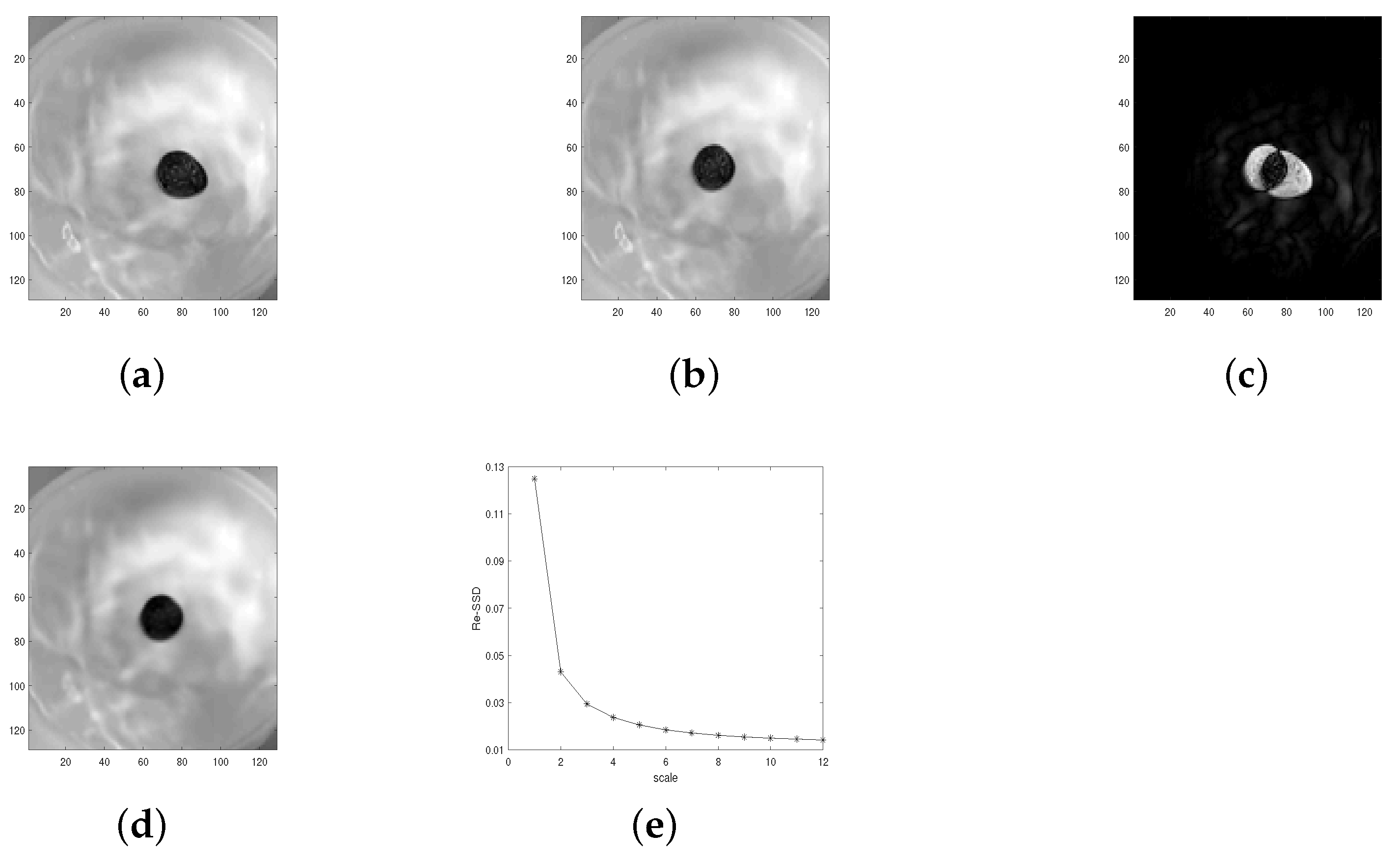
4. Numerical Tests

In this section, we use several numerical tests to demonstrate the good performance of the proposed multiscale approach. All the numerical tests were implemented under Windows 10 and Matlab R2019a with 11th Gen Intel(R) Core(TM) i5-1135G7 @ 2.40 GHz and 16.0 GB memory. For this purpose, we compared the proposed multiscale approach with the BD model in [12], LDDMM-demons algorithm in [33], and TV model in [30] to validate the efficiency of the multiscale approach. In particular, the BD model can be viewed as a single scale approach without iteration (scale = 1). The used data sets included synthetic images, medical images, and underwater distorted images. The comparison between the BD model and the proposed multiscale approach helps to validate the fact that the proposed approach has advantages in getting out of the local minimum of the object functional. The size of all images used for registration is $129\times 129$. In order to evaluate the similarity between the deformed source image and target image, we used the relative sum of squared difference to quantitatively evaluate the registration results. The relative sum of squared difference is defined as follows:

$$Re-SSD(T,D,\mathbf{u})=\frac{SSD\left(T\right(\mathbf{x}+\mathbf{u}),D)}{SSD(T,D)},$$

(26)

where $SSD(T,D)=\frac{1}{2}{\sum }_{i,j}{(T_{i,j}-D_{i,j})}^2$.

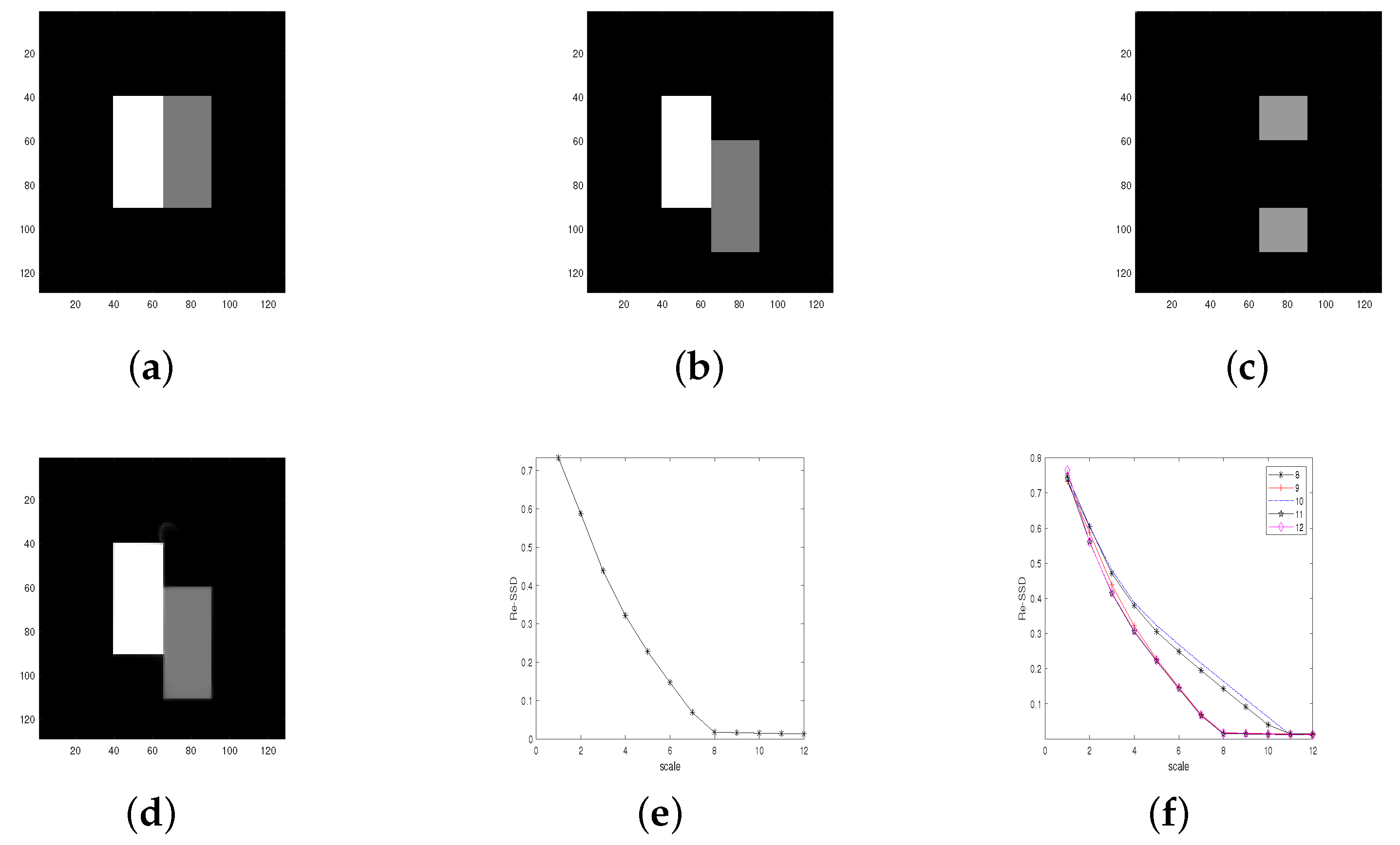
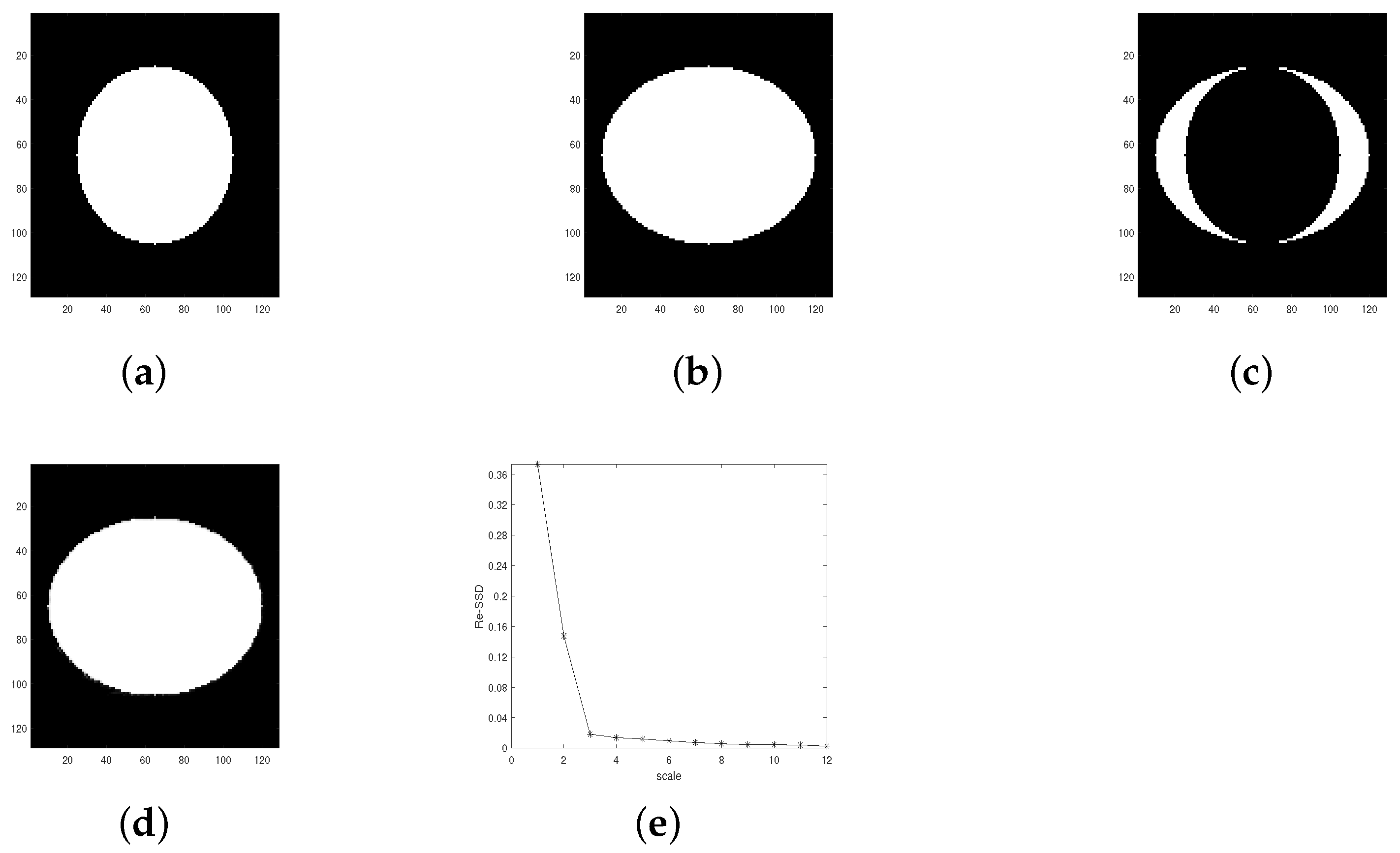
Test 1 (Test for synthetic images) In this test, we presented two numerical tests by comparing these four algorithms: proposed multiscale approach (Algorithm 2), BD model algorithm in [12], the LDDMM-demons algorithm in [33], and TV model in [30]. These two tests were performed on synthetic image pairs, Rectangle and C-E, respectively. By using these four different algorithms to register the above two image pairs, respectively, we list the registration results in Figure 1, Figure 2, Figure 3 and Figure 4 and

Table 1. Quantitative comparison of registration results of four different algorithms (test for synthetic image pairs).

Data	Algorithm	Re-SSD (%)	CPU/s
Rectangle	Proposed	1.3	213
	BD	71	16.8
	LDDMM	18.74	143
	TV	31.56	249.3
C-E	Proposed	0.27	83.7
	BD	0.78	20.7
	LDDMM	3.15	101.8
	TV	4.29	210.2

. Moreover, sensitivity tests for parameter ${\mathsf{\Theta }}_n$ are also listed in Figure 1. One can notice that from Figure 1f, the final registration result is not sensitive to the parameter, while ${\mathsf{\Theta }}_n$ and ${\mathsf{\Theta }}_n$ only affects the convergence speed. This coincides with the result in [25]. In Figure 2 and Figure 4, we can see that $S_n\left(\mathbf{u}\right)$ gradually decreases with respect to the scale number n. In addition, the final $Re-SSD$ achieves 1.3% and 0.27%, respectively. This indicates $T\circ {\widehat{\mathbf{h}}}_{K_M}(·)\approx D(·)$, which implies that the proposed multiscale approach leads to an accurate result. 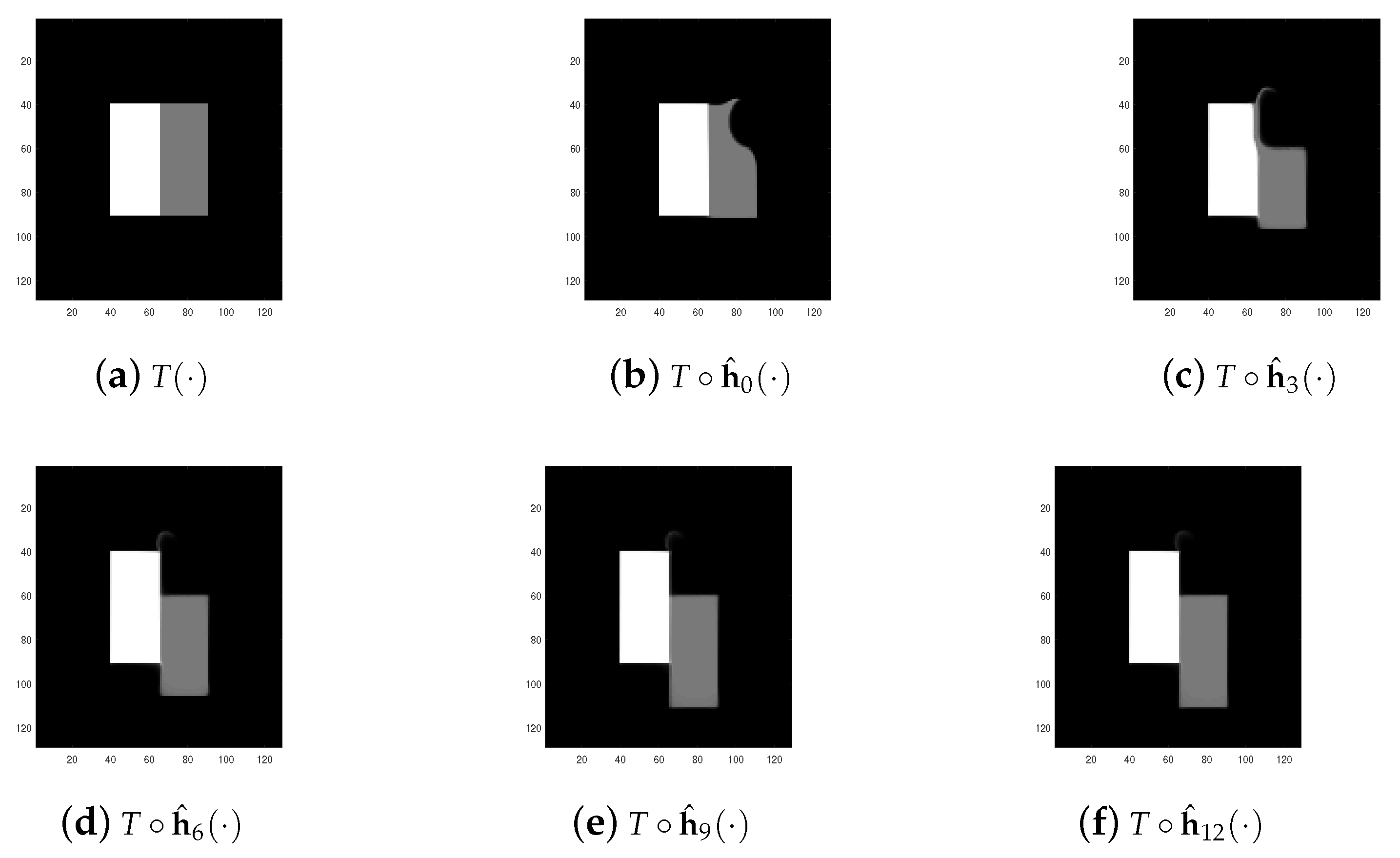With the quantitative comparison results in Table 1, we obtain the following two conclusions: (I) The proposed multiscale approach has advantages in overcoming the local minimum of the object functional. In fact, in the comparison between the BD model and the proposed algorithm, we see that the proposed Algorithm 2 obviously improves the registration result. Moreover, one can notice that the final $Re-SSD$ for the BD model on the Rectangle image pair is 71%. This shows that the algorithm in [12] is trapped into a local minimum. Compared with $Re-SSD=71\%$ led by the local minimum, the proposed Algorithm 2 achieves a very good result with 1.3%. This validates the fact that the proposed Algorithm 2 has advantages on overcoming the local minimum of the object functional. This is also the main motivation for this work. 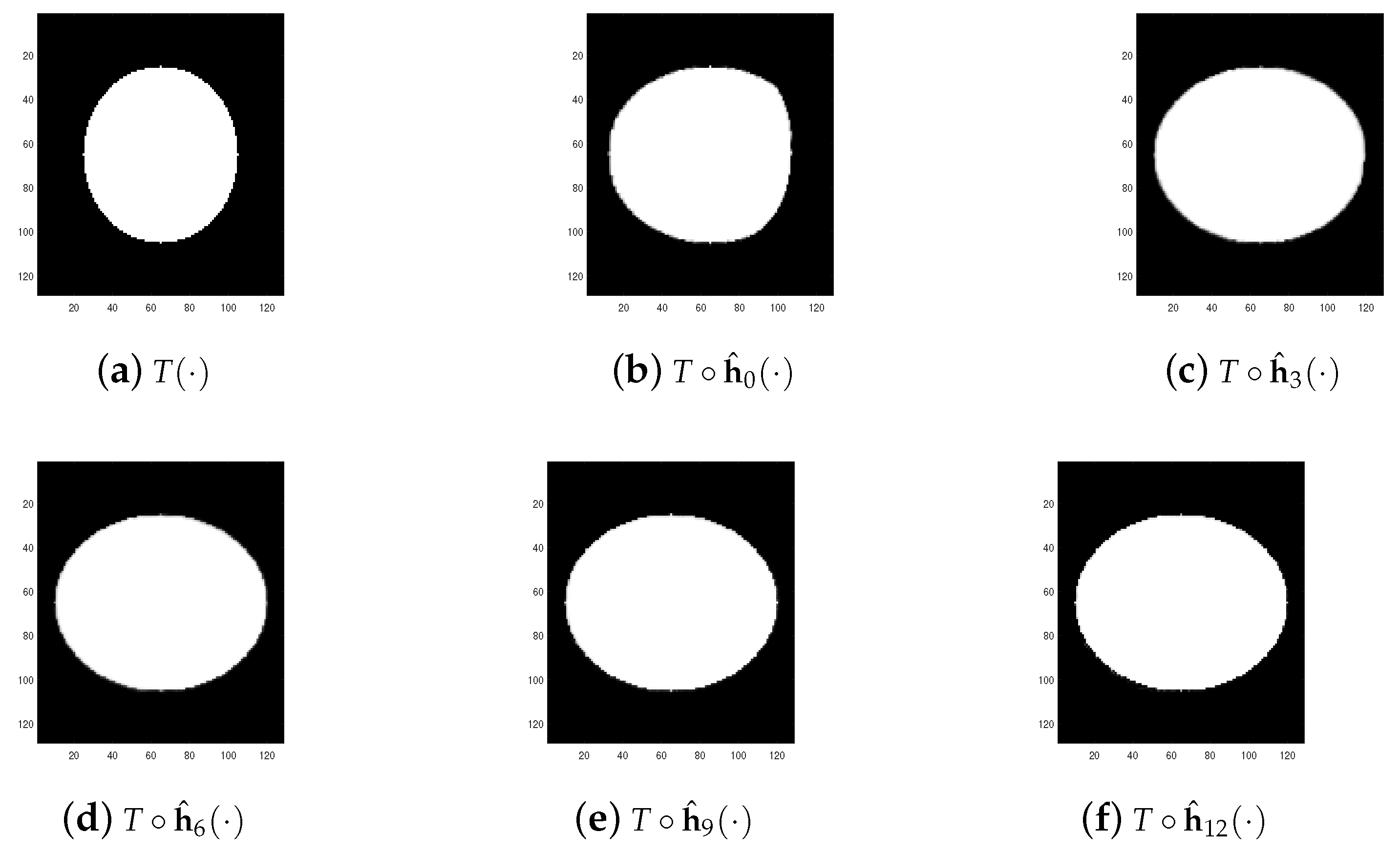In addition, the final $Re-SSD$ of image pair C-E($Re-SSD=0.27\%$) shows that the proposed Algorithm 2 can also address the smooth registration well (note that C-E induces a continuous deformation). At last, with Figure 1e and Figure 3e, we can conclude the sequence $S_n\left(\mathbf{u}\right)$ converges as $n\to \infty$. This validates that the proposed Algorithm 2 induces a convergence similarity sequence. This coincides with the conclusion at the end of Section 2. (II) The proposed Algorithm 2 addresses the discontinuous registration well. One can notice that the image pair Rectangle induces a discontinuous deformation (this is the main reason why this image pair is selected for numerical comparison). It follows from Table 1 that the three discontinuous methods (Algorithm 2, BD model, TV model) obviously perform much better than the diffeomorphic model (LDDMM). Moreover, one can also see that the proposed Algorithm 2 achieves the smallest $Re-SSD$. This shows that the proposed Algorithm 2 is competitive to some state-of-the-art registration algorithms.

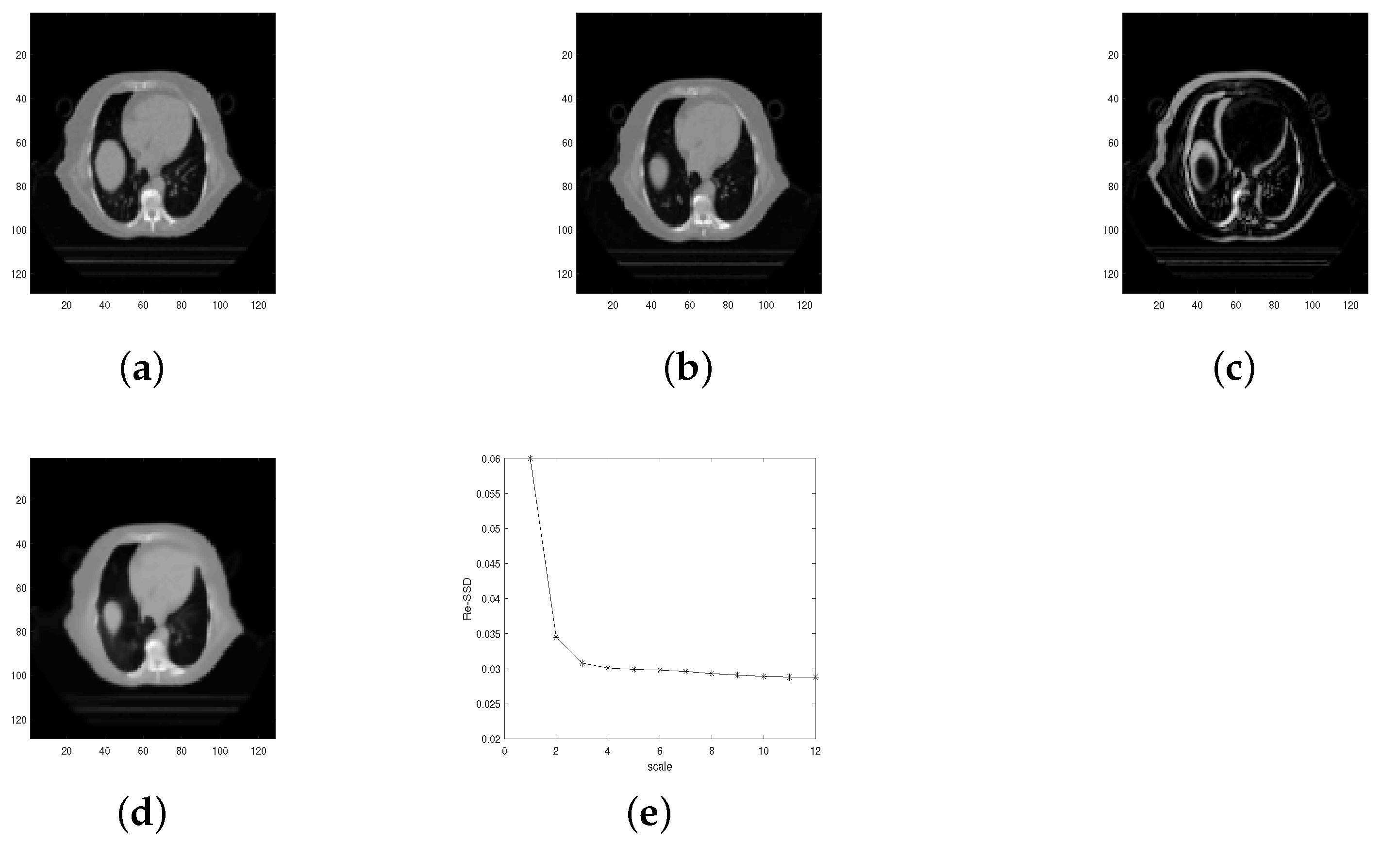
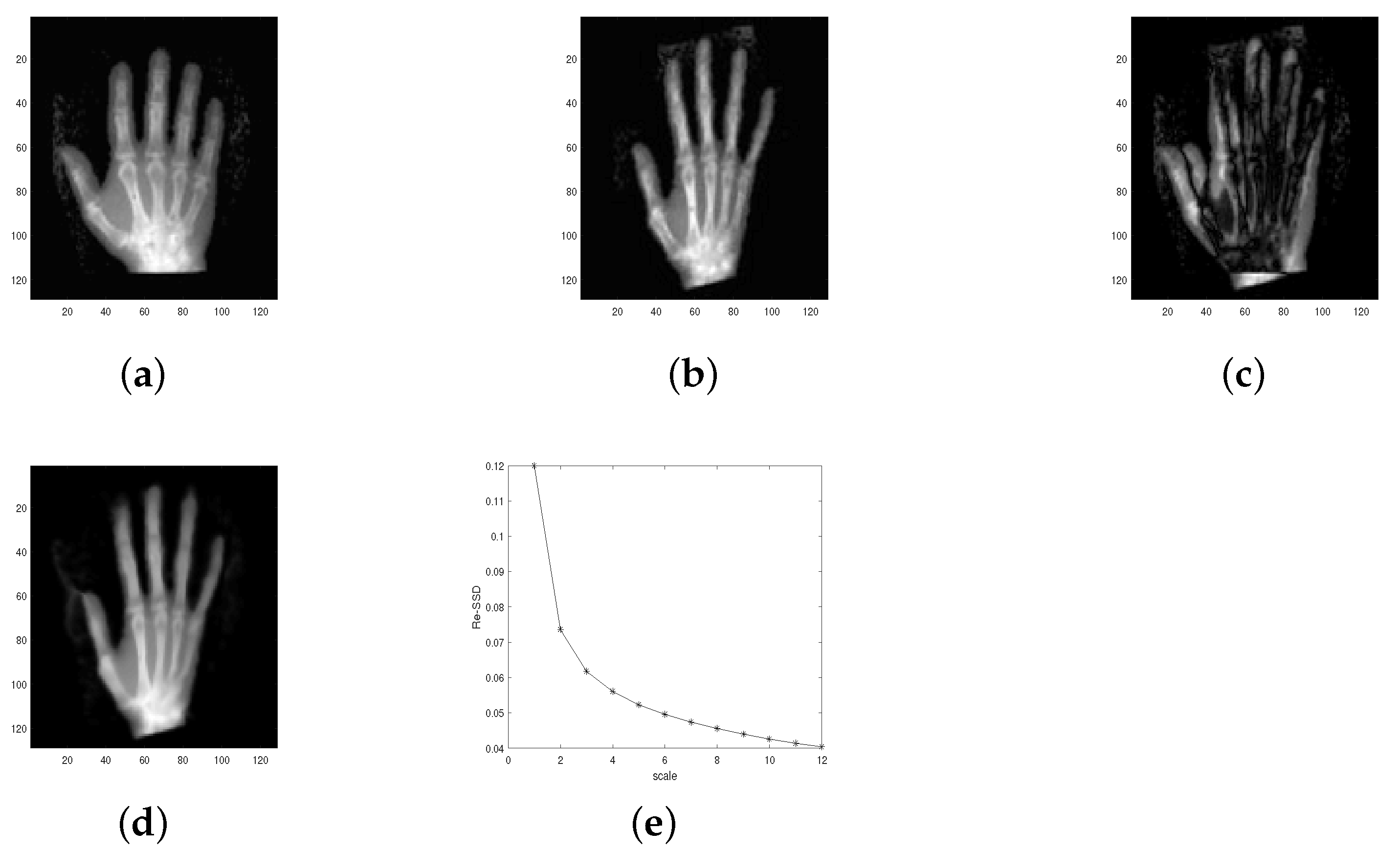
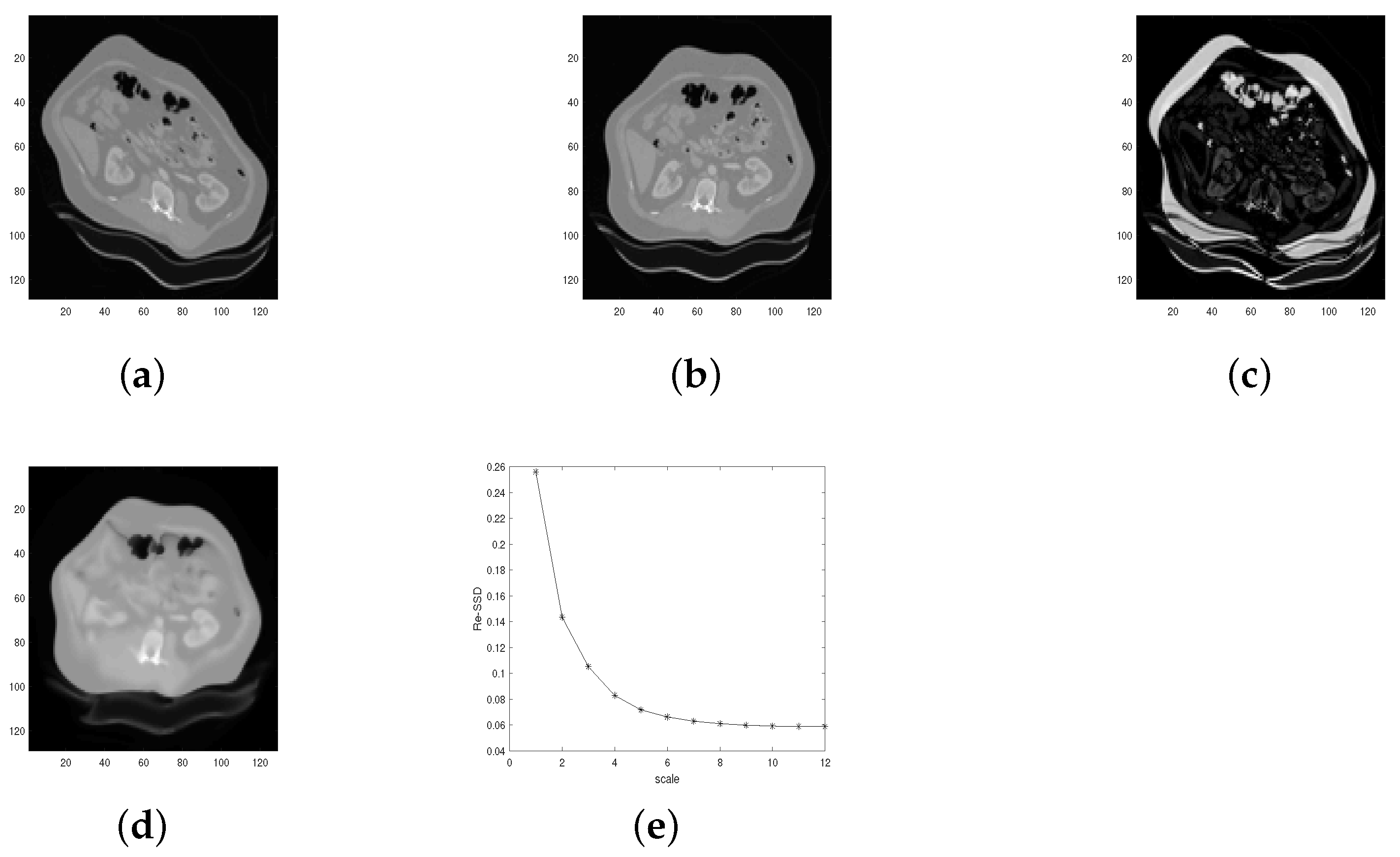
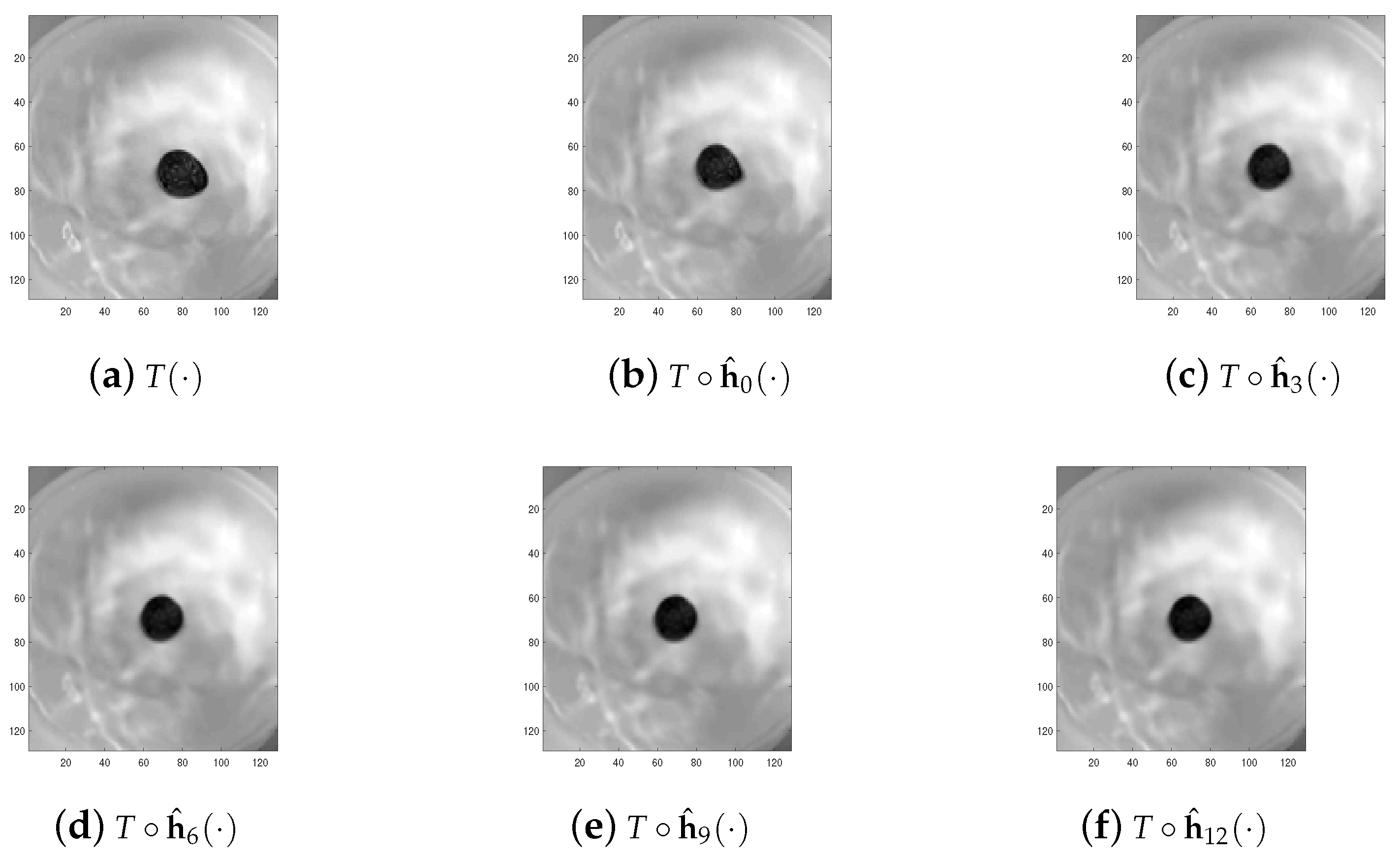
Test 2 (Test for medical images) Similar to Test 1, we used Algorithm 2, the BD model algorithm in [12], the LDDMM-demons algorithm in [33], and the TV model in [30] to register three different kinds of medical image pairs: lung, hand, and liver. The final registration results are listed in Figure 5, Figure 6, Figure 7, Figure 8, Figure 9 and Figure 10 and

Table 2. Quantitative comparison of registration results of four different algorithms (test for medical image pairs).

Data	Algorithm	Re-SSD (%)	CPU/s
Lung	Proposed	2.88	102.8
	BD	6.73	15.9
	LDDMM	5.55	123.2
	TV	4.63	98.3
Hand	Proposed	4.04	195.7
	BD	8.3	19.8
	LDDMM	5.99	114.9
	TV	8.83	112.2
Liver	Proposed	5.88	119.75
	BD	16.85	8.6
	LDDMM	15.14	118.5
	TV	19.6	630.3

. With Figure 5e, Figure 7e and Figure 9e, we conclude that the proposed multiscale approach plays an important role in overcoming the local minimum. On the other hand, in Figure 5d, Figure 7d and Figure 9d, we see that the final registration result $T\circ {\widehat{\mathbf{h}}}_{K_M}(·)$ looks nearly the same with the target image $D(·)$. This shows the high accuracy of the proposed Algorithm 2 in view of computer vision. Concerning the quantitative comparison between the BD model and the proposed multiscale approach, it follows from Table 2 that the proposed multiscale approach obviously improves the result of the BD model, though it costs much more CPU time. Note that here we care more about the registration result rather than the CPU time. Particularly, the final result ($Re-SSD=16.85\%$) of the BD model demonstrates that the BD model gets into a local minimum of the object functional. This is mainly caused by the nonconvexity of the object functional. 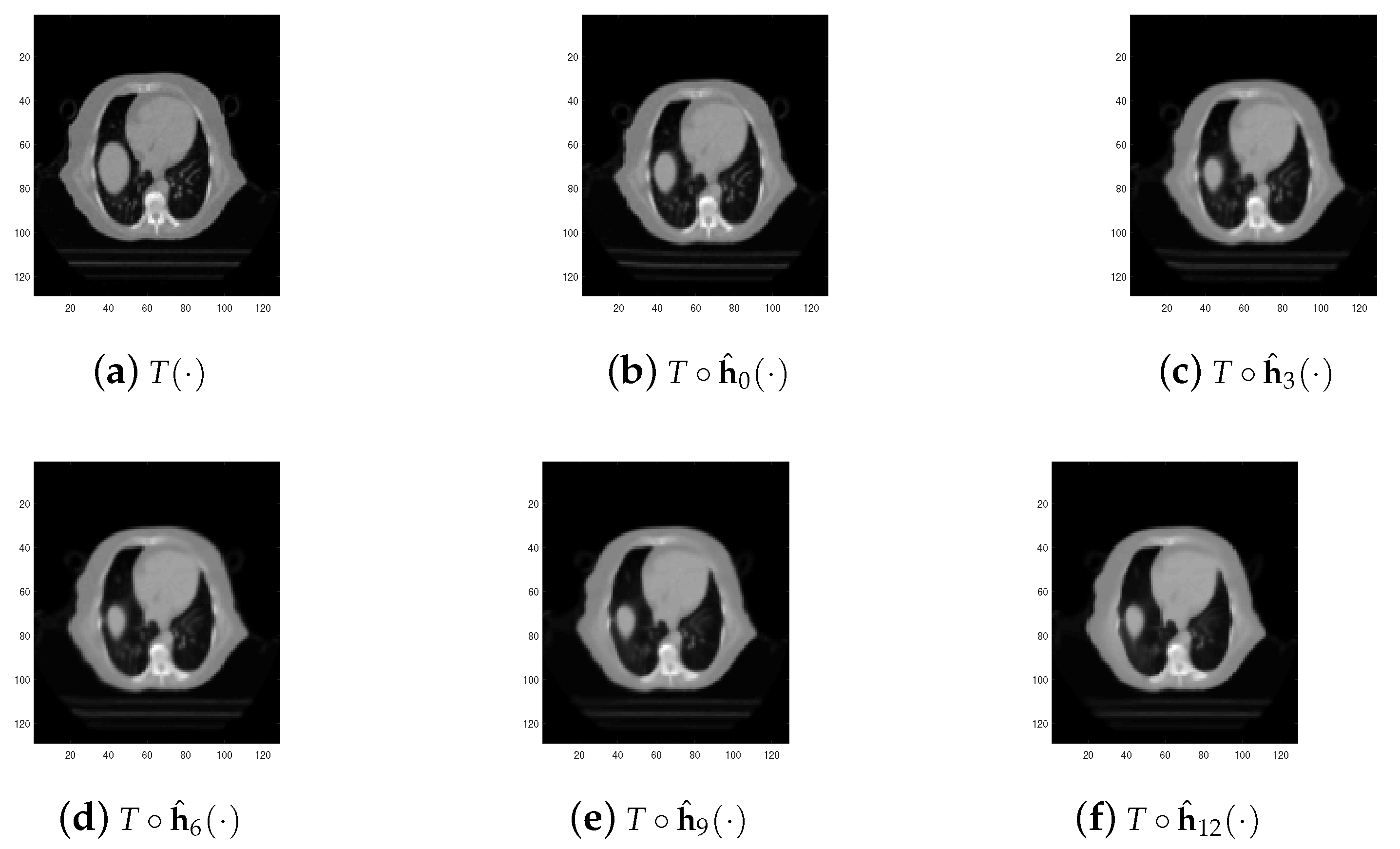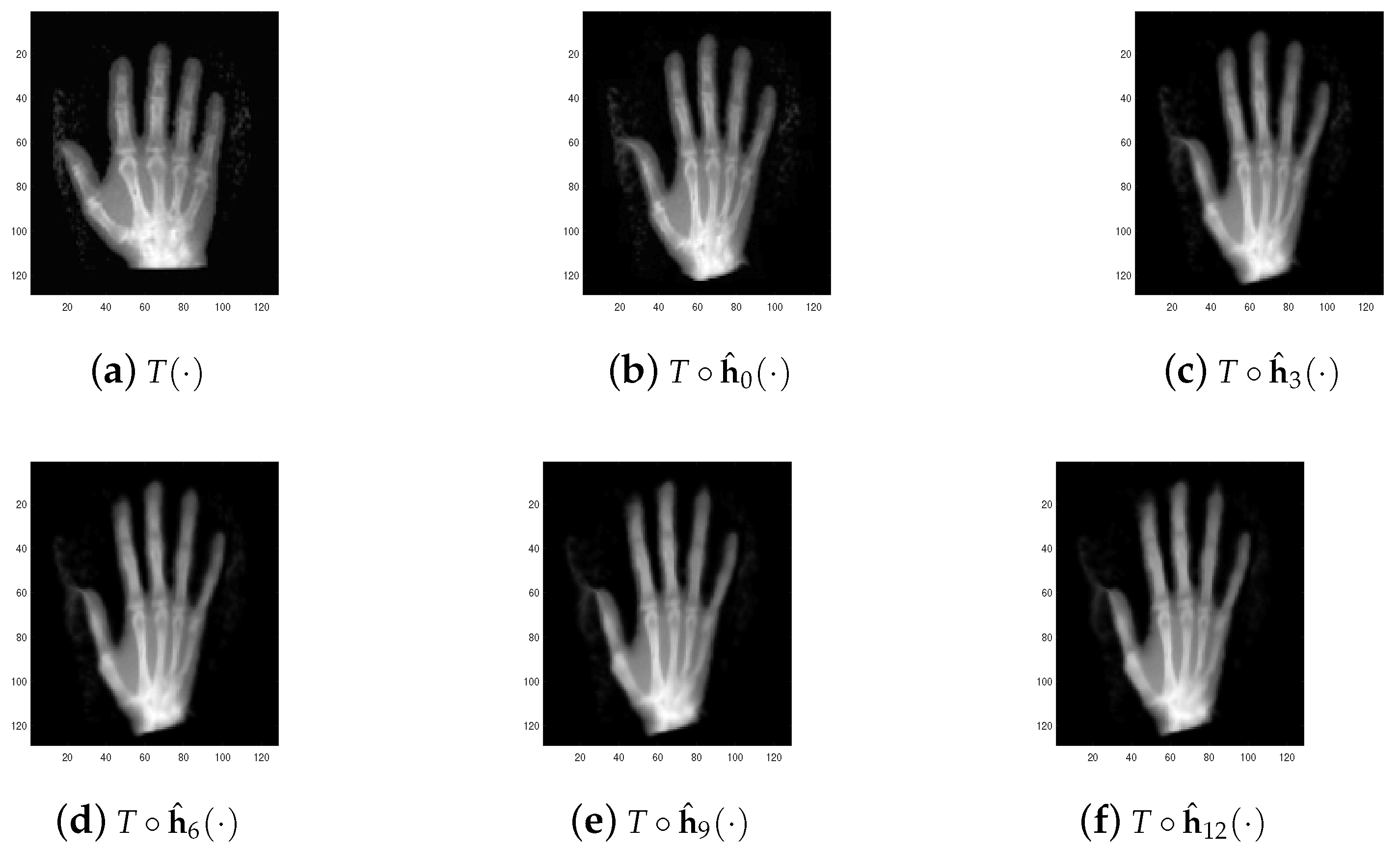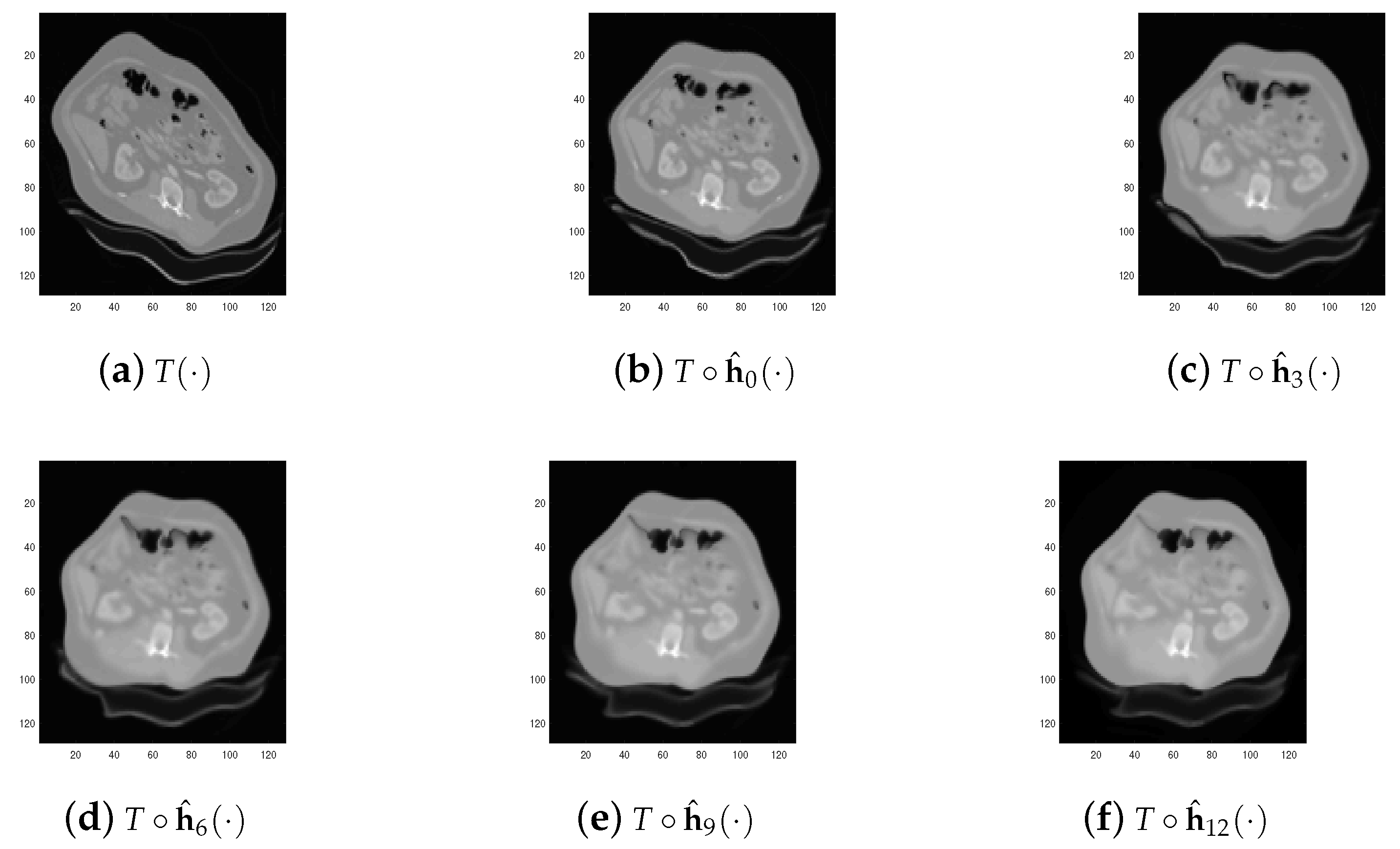A sharp contrast to this result, the final registration result ($Re-SSD=5.88\%$) for the proposed Algorithm 2 shows that the proposed approach can effectively improve the final registration results. Concerning the process for the details of improvement, one can see Figure 6, Figure 8 and Figure 10. In addition, through the quantitative comparison results in Table 2, we see that the proposed Algorithm 2 is competitive to the other three registration algorithms. Moreover, one can see that the BD model achieves the worst result among these four algorithms, while the BD-based multiscale approach achieves the best image registration result. This further validates the fact that the proposed approach has advantages in overcoming the local minimum of the object functional.

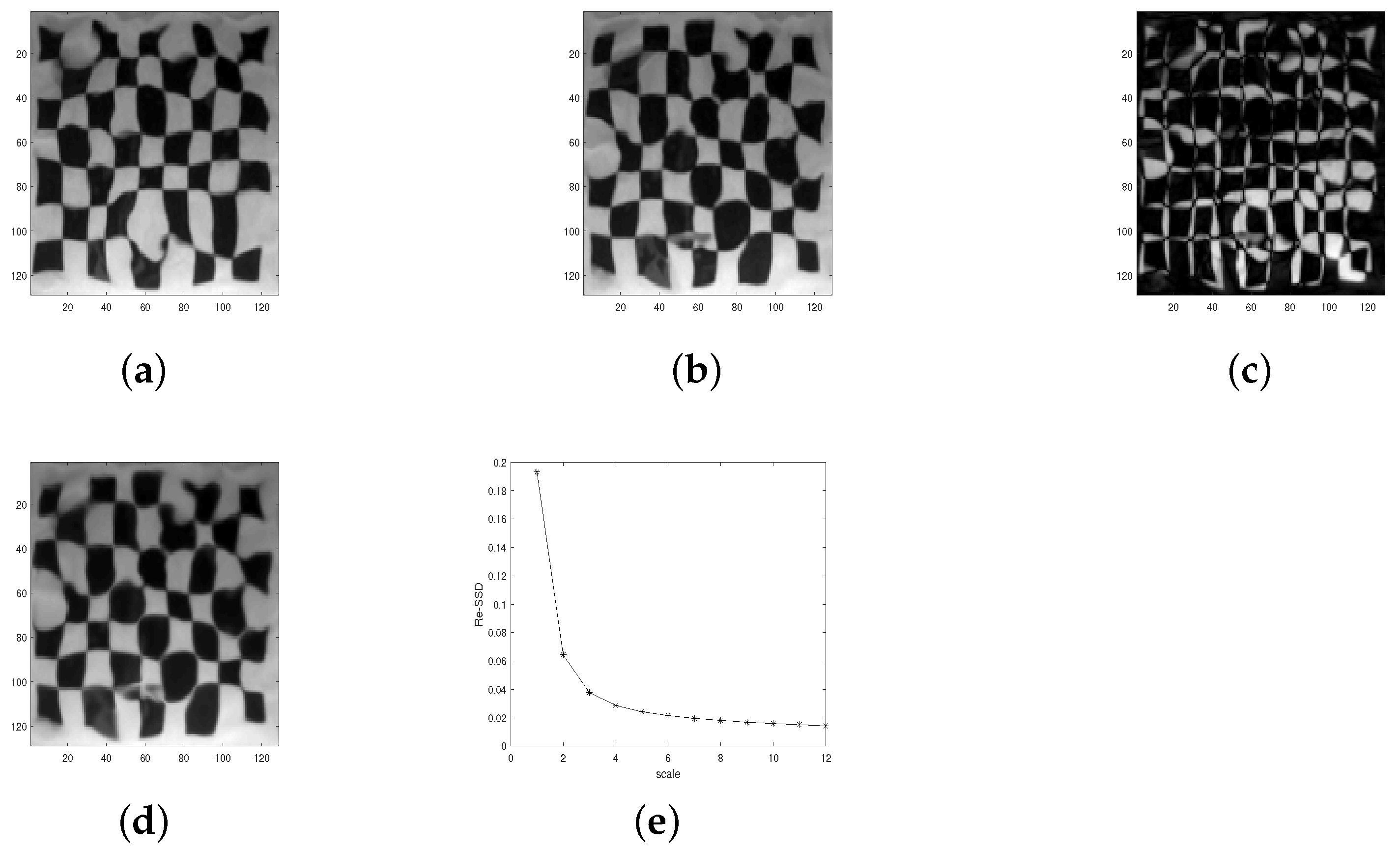
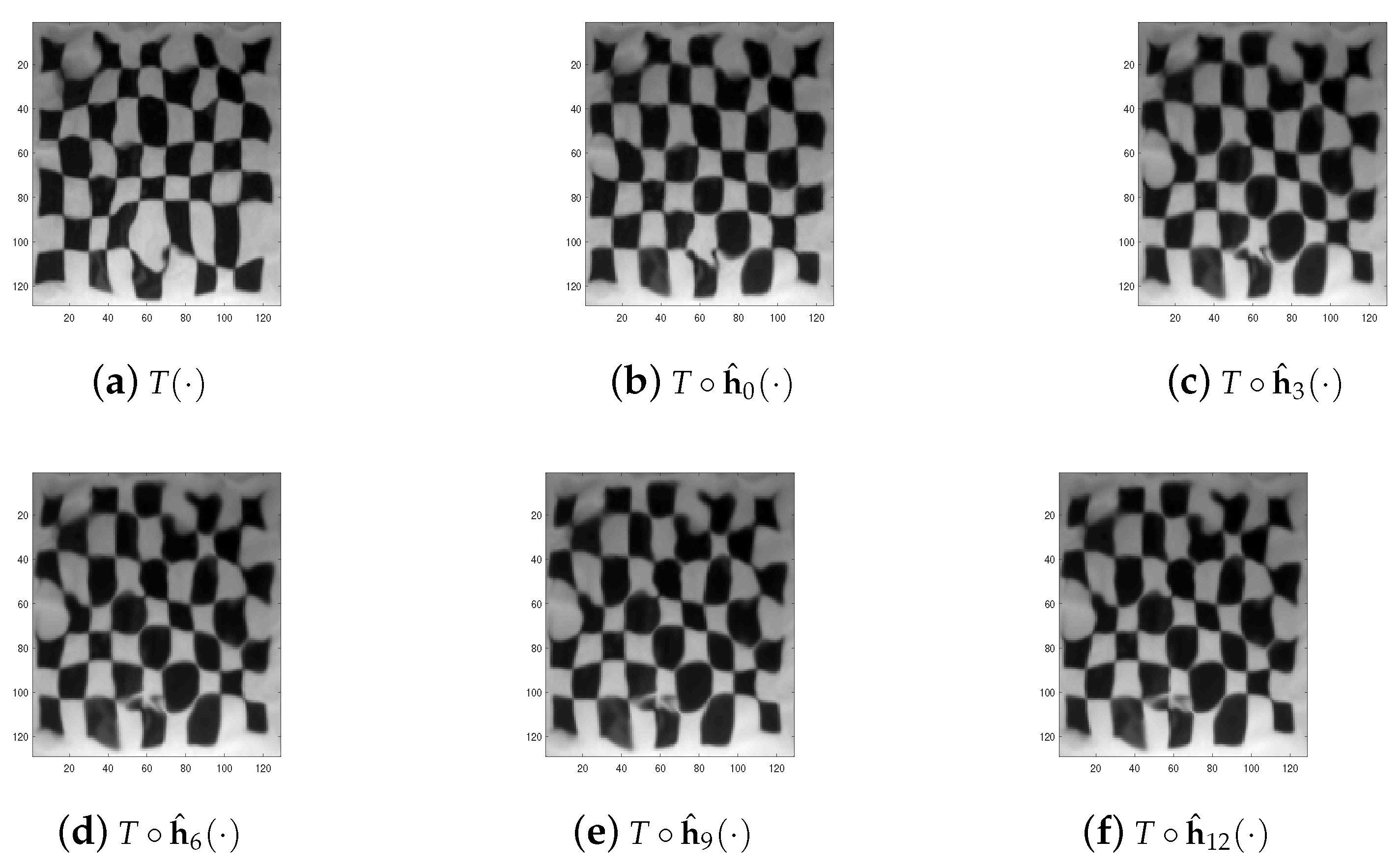
Test 3 (Test for underwater images) At the end of this section, we test the proposed Algorithm 2 on very special natural image pairs: underwater images. In underwater images, serious distortion occurs, which makes it difficult for image registration. In this test, we selected two image pairs (Square and Coin) as experimental data. We used Algorithm 2, the BD model algorithm in [12], the LDDMM-demons algorithm in [33], and the TV model in [30] to register these two image pairs, and the final registration results are listed in Figure 11, Figure 12, Figure 13 and Figure 14 and

Table 3. Quantitative comparison of registration results of four different algorithms (test for underwater distorted image pairs).

Data	Algorithm	Re-SSD (%)	CPU/s
Square	Proposed	1.43	242.4
	BD	8.28	8.5
	LDDMM	8.86	20.6
	TV	2.99	244.7
Coin	Proposed	1.42	272.65
	BD	6.95	22.2
	LDDMM	58.99	248
	TV	97.83	213.14

. In Figure 11e and Figure 13e, we see that the $S_n\left(\mathbf{u}\right)$ induced by proposed the multiscale approach converges to the global minimum of $S\left(\mathbf{u}\right)$ on $\mathcal{K}$. Additionally, with Figure 11d and Figure 13d, we know that the deformed image $T\circ {\widehat{\mathbf{h}}}_{K_M}(·)$ induced by the proposed Algorithm 2 looks the same with target image $D(·)$. At last, one can see from Table 3 that the proposed multiscale approach achieves the best result among the four comparison results. This shows the high accuracy of the proposed algorithm. Moreover, via comparison through data Coin, we see that the LDDMM and TV model are trapped in the local minimum for some default parameters, while the local minimum does not occur in all the numerical tests performed by the proposed Algorithm 2. This validates the fact that the proposed Algorithm 2 is robust and independent of parameters.

Analysing the registration results of these three tests, we conclude that the proposed Algorithm 2 has the advantage of improving the registration results for different kinds of image pairs (i.e., natural iamge and medical image). Moreover, via the relationship between $Re-SSD$ and scale number listed in these three tests, we also conclude that the proposed Algorithm 2 can help to overcome the local minimum of the object functional and make the registration more accurate.

5. Conclusions and Discussion

In this paper, we propose a multiscale approach for the BD model, which addresses the discontinuous registration well. By setting an increasing sequence ${\mathsf{\Theta }}_n$ in the multiscale approach, we show that the similarity sequence $\left\{S_n\left(\mathbf{u}\right)\right\}$ converges to the global minimum of the original similarity. A numerical algorithm is also presented to simulate the multiscale approach. Based on the proposed algorithm, several numerical tests are performed to validate the main motivation for this paper: (I) Overcoming the local minimum of the similarity; (II) Addressing the discontinuous registration caused by strong noise or pathological tissue.

For future research, one could try to extend the 2D image registration into 3D multiscale image registration. The study of 3D image registration is a very important topic. This makes it possible for clinical application and diagnosis.