Discretization, Bifurcation, and Control for a Class of Predator-Prey Interactions

Abstract

The present study focuses on the dynamical aspects of a discrete-time Leslie-Gower predator-prey model accompanied by a Holling type III functional response. Discretization is conducted by applying a piecewise constant argument method of differential equations. Moreover, boundedness, existence, uniqueness, and a local stability analysis of biologically feasible equilibria were investigated. By implementing the center manifold theorem and bifurcation theory, our study reveals that the given system undergoes period-doubling and Neimark-Sacker bifurcation around the interior equilibrium point. By contrast, chaotic attractors ensure chaos. To avoid these unpredictable situations, we establish a feedback-control strategy to control the chaos created under the influence of bifurcation. The fractal dimensions of the proposed model are calculated. The maximum Lyapunov exponents and phase portraits are depicted to further confirm the complexity and chaotic behavior. Finally, numerical simulations are presented to confirm the theoretical and analytical findings.

1. Introduction

predator-prey models have a wide range of applications in ecological and biological fields. Although various fundamental aspects of the nonlinear dynamics of predator-prey population models related to continuous dynamical systems have been studied, the characteristics of discrete dynamical systems remain comparatively unknown. A discrete dynamical structure possesses a solitary dynamical nature as compared to a continuous system. There are several critical and practical problems in daily life that can be characterized with the help of a discrete dynamical system. To consider the analytical aspects of a solution that is difficult to calculate, various schemes can be implemented to discretize a continuous system and discuss the numerical solution. Therefore, detailed critical inspections of discrete-time dynamical systems have contributed immensely to various fields such as engineering, physics, chemistry, and mathematics. There have been numerous studies conducted that are related to the dynamics of predator-prey models.

Chen et al. [1] applied the Euler scheme and center manifold theorem to a ratio-dependent prey-predator model and scrutinized the dynamic characteristics of the model. Ghaziani et al. [2] studied a prey-predator system with a Holling functional response and discussed the resonance and bifurcation analyses. Jana [3] found extremely powerful dynamical conditions through numerical and theoretical investigations of discrete-time prey-predator models, such as stability conditions, flip, and hopf-bifurcation. Misra et al. [4] studied a predator-prey model based on age predation and discussed the dynamic behavior of the models. Zhang et al. [5] presented a biological economic system related to the predator-prey model of a differential algebraic system by applying a new normal form. Hu and Cao [6] investigated the Holling and Leslie type predator-prey model and discussed a chaos and bifurcation analysis. Wang and Li [7] proposed a lemma that is extremely meaningful for discussing the stability and bifurcation of the systems. The fundamental finding in the dynamics of prey-predator species is the classical Lotka-Volterra prey-predator model, which exhibits unrealistic behavior (see, Murdoch et al. [8]). To remove such unrealistic behavior, Holling introduced three different types of functional responses (see, Holling [9]). Rosenzweig and MacArthur [10] implemented a functional response to modify the predator-prey model. An investigation into population interaction focused on the continuous dynamical system of two species [11,12,13]. By contrast, a recent study led to the discrete dynamical system becoming more suitable than a continuous version when the population is non-overlapping (e.g., see, Jing et al. [14], Liu et al. [15], Lopez-Ruiz and Fournier-Prunaret [16], Neubert and Kot [17]). Furthermore, multiple existing studies related to the dynamics of predator-prey models are described in [18,19,20,21,22,23,24,25,26]. In [27], the Holling type-III functional response was introduced in both populations (prey and predator). The stability conditions around biologically suitable equilibria were further discussed. Diagrams of the phase portraits, bifurcation, and time series were plotted. It was shown that the system is sensitive to the initial conditions, which means that the system is chaotic. A two-dimensional continuous model with a Holling-III functional response in both prey and predator was presented [28]. Furthermore, Euler’s scheme was used to discretize the model and study the complex behavior of the system. Elettreby et al. [29] discussed a discrete-time prey-predator model with predator and prey populations having Holling type I and III functional responses, respectively. Moreover, they described a fascinating dynamical nature of the model, including stability, bifurcation, and chaos, which ensure the rich dynamics of discrete-time models.

In this study, we evaluate the specific prey –predator model discussed by Murray [30]:

$$\begin{array}{ll}\hfill \frac{dx}{dt}=& x\left[r\left(1-\frac{x}{k}\right)-\frac{axy}{b^2+x^2}\right],\hfill \\ \hfill \frac{dy}{dt}=& ys\left(1-\frac{hy}{x}\right),\hfill \end{array}$$

(1)

where $x\left(t\right)$ and $y\left(t\right)$ denote the densities of prey and predator species at any time $t$, respectively; the carrying capacity of prey in the absence of predator is $k$, and $r, b, a, s,\mathrm{and}h$ are positive constants. Moreover, the carrying capacity is proportional to the prey population size and population of prey attacked by predators, as specified by the Holling type III functional response. He and Lai [31] examined the bifurcation and chaos control of the discrete-time version of model (1) by implementing Euler’s forward scheme with step size $h$ as the bifurcation parameter. The numerical results in [31] show that period-doubling bifurcation occurs when a large step size is considered in Euler’s method; this fact contravenes the precision of the numerical method for discretization. To overcome this deficiency, the following discretization method was implemented. Considering the regular time interval for the average growth rate in both populations, by resorting to piecewise constant arguments for solving nonlinear differential equations, system (1) can then be rewritten as follows:

$$\begin{array}{ll}\hfill \frac{1}{x\left(t\right)}\frac{dx\left(t\right)}{dt}=& \left[r\left(1-\frac{x\left[t\right]}{k}\right)-\frac{ax\left[t\right]y\left[t\right]}{b^2+x{[t]}^2}\right],\hfill \\ \hfill \frac{1}{y\left(t\right)}\frac{dy\left(t\right)}{dt}=& s\left(1-\frac{hy\left[t\right]}{x\left[t\right]}\right),\hfill \end{array}$$

(2)

where the integer part of $t$ is given by $\left[t\right]$ within the interval $0<t<1$. In addition, by integrating system (1) for $t\in \left[n:n+1\right]$, ($n=0,1,2,\dots$), we have the following system:

$$\begin{array}{ll}\hfill x\left(t\right)=& x_n\exp \left(\left[r\left(1-\frac{x_n}{k}\right)-\frac{a{x}_n{y}_n}{b^2+x_n{}^2}\right]\left(t-n\right)\right),\hfill \\ \hfill y\left(t\right)=& y_n\exp \left(\left[s\left(1-\frac{h{y}_n}{x_n}\right)\right]\left(t-n\right)\right).\hfill \end{array}$$

(3)

Applying $t\to n+1$, we obtain the following prey-predator system:

$$\begin{array}{ll}\hfill x_{n+1}=& x_n\exp \left(r\left(1-\frac{x_n}{k}\right)-\frac{a{x}_n{y}_n}{b^2+x_n{}^2}\right),\hfill \\ \hfill y_{n+1}=& y_n\exp \left(s\left(1-\frac{h{y}_n}{x_n}\right)\right).\hfill \end{array}$$

(4)

The key contributions and findings of the current study are as follows for model (4):

• The existence and uniqueness of biologically feasible equilibria and their stability analysis are discussed.
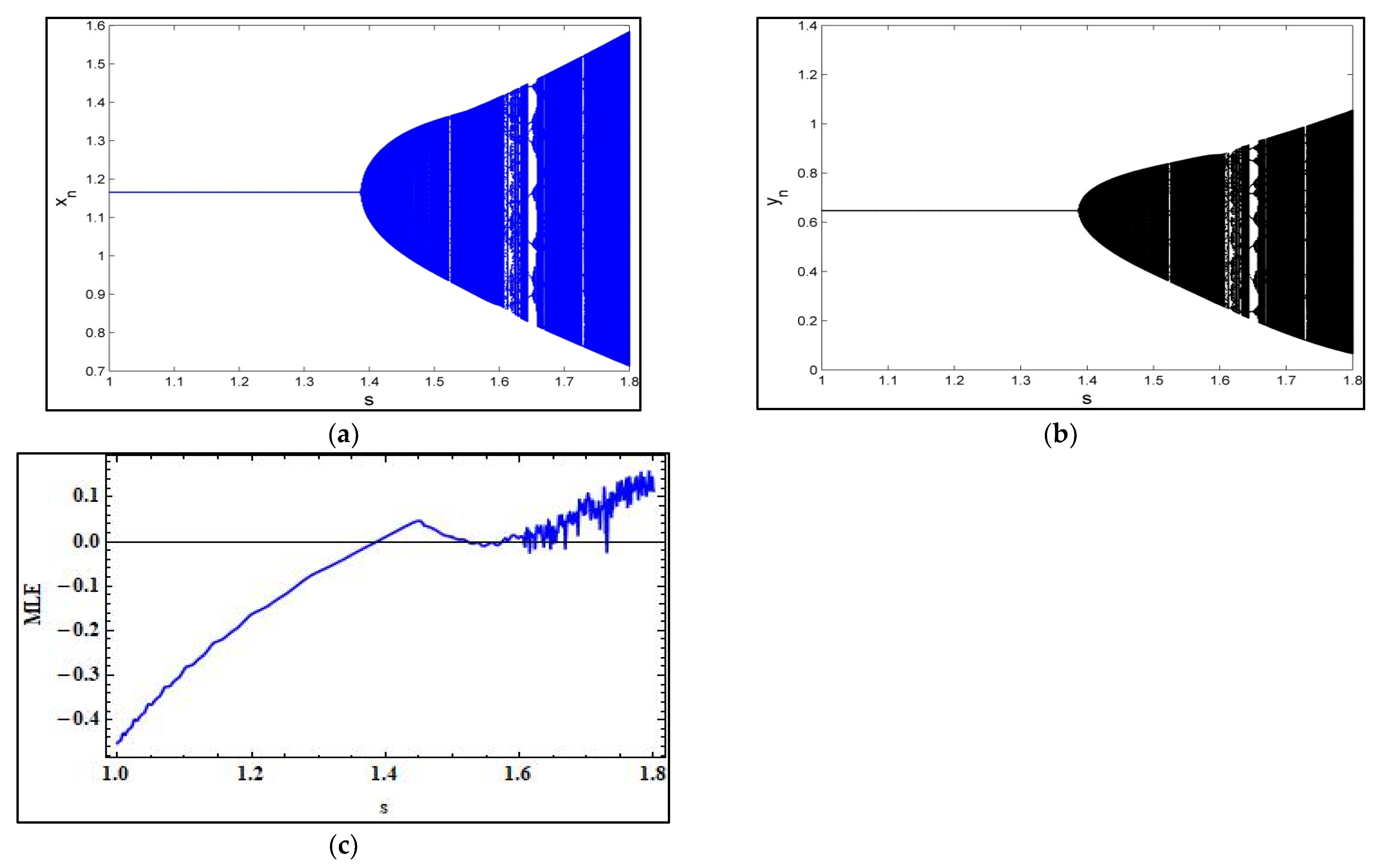
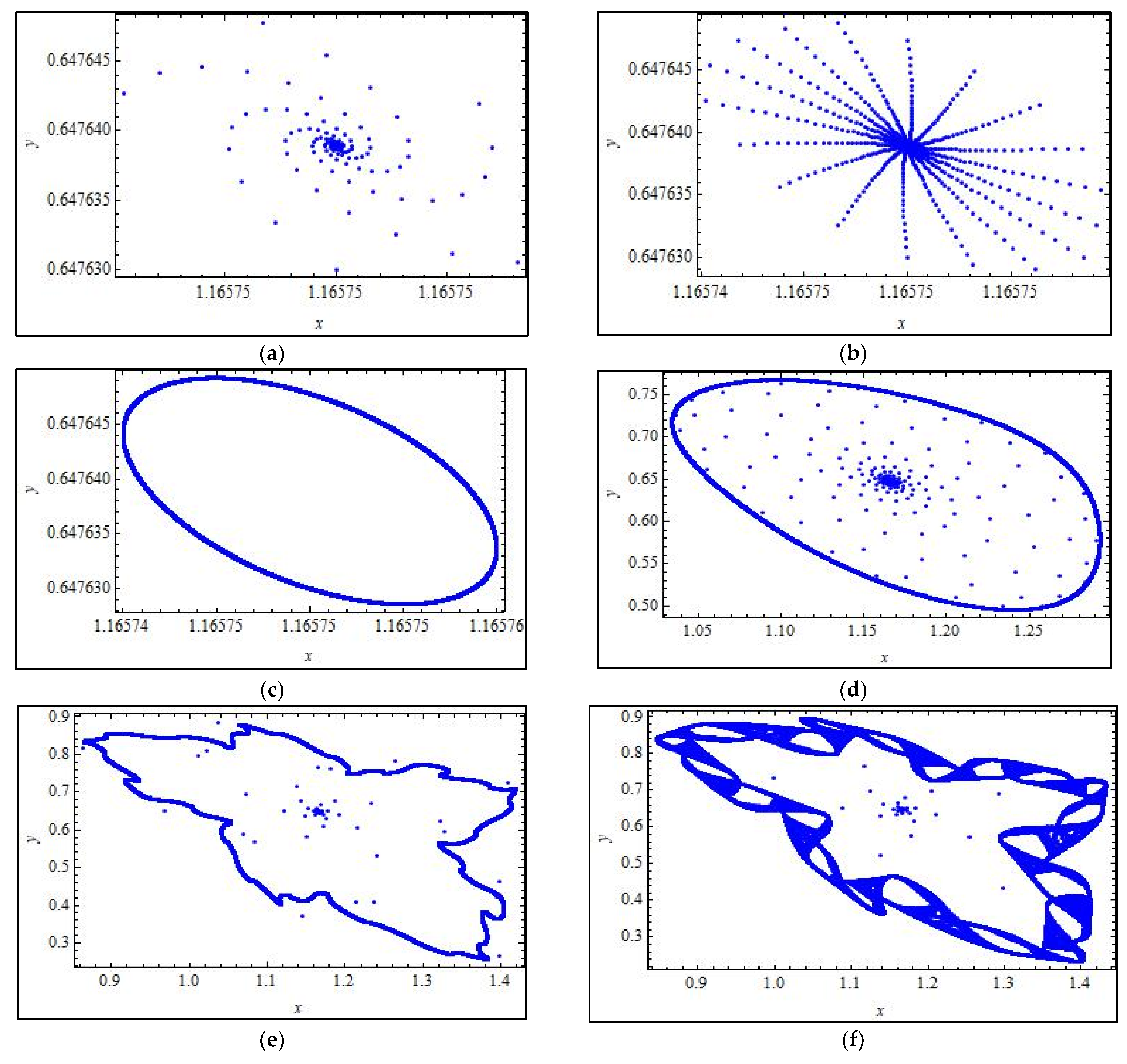
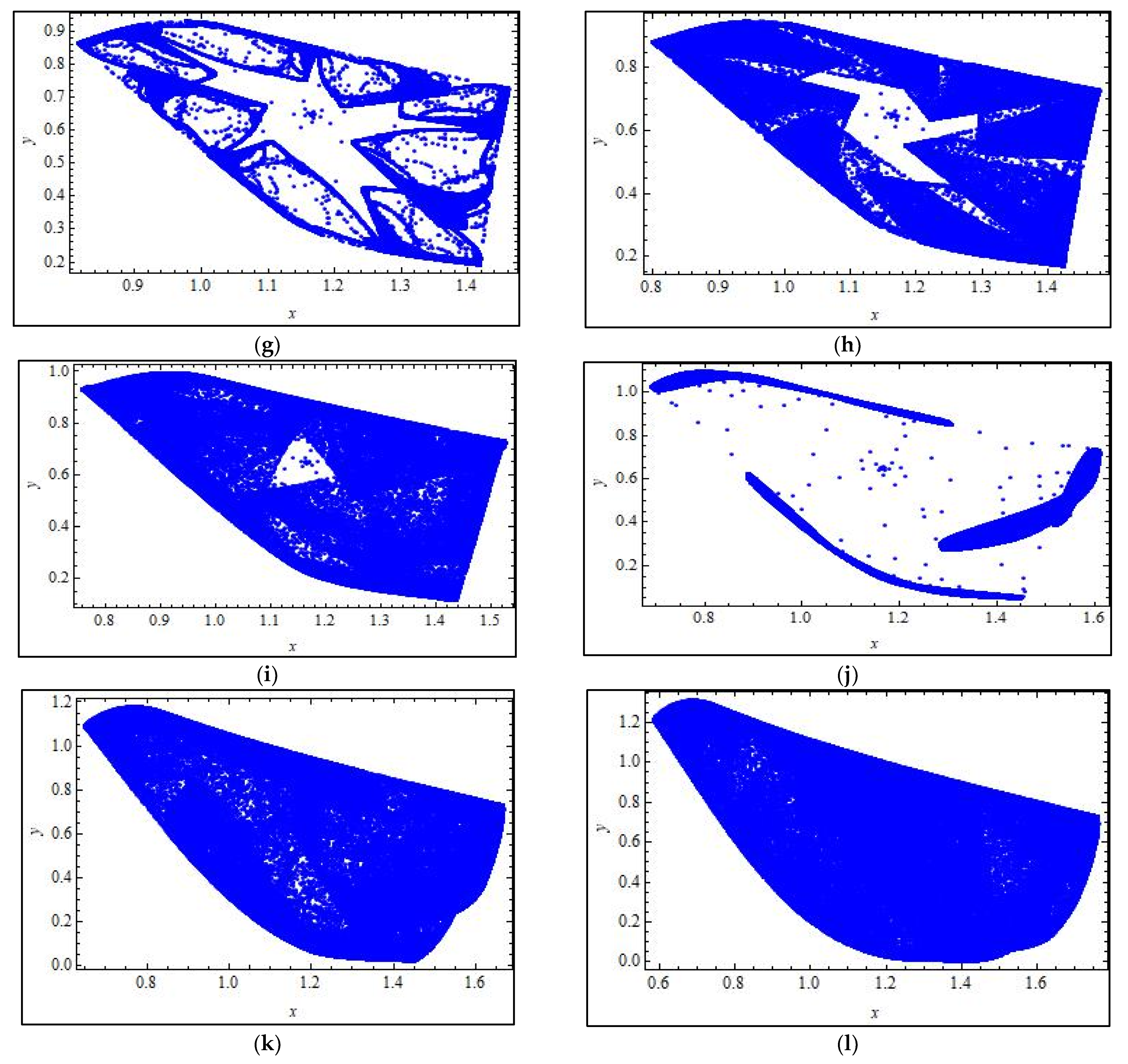
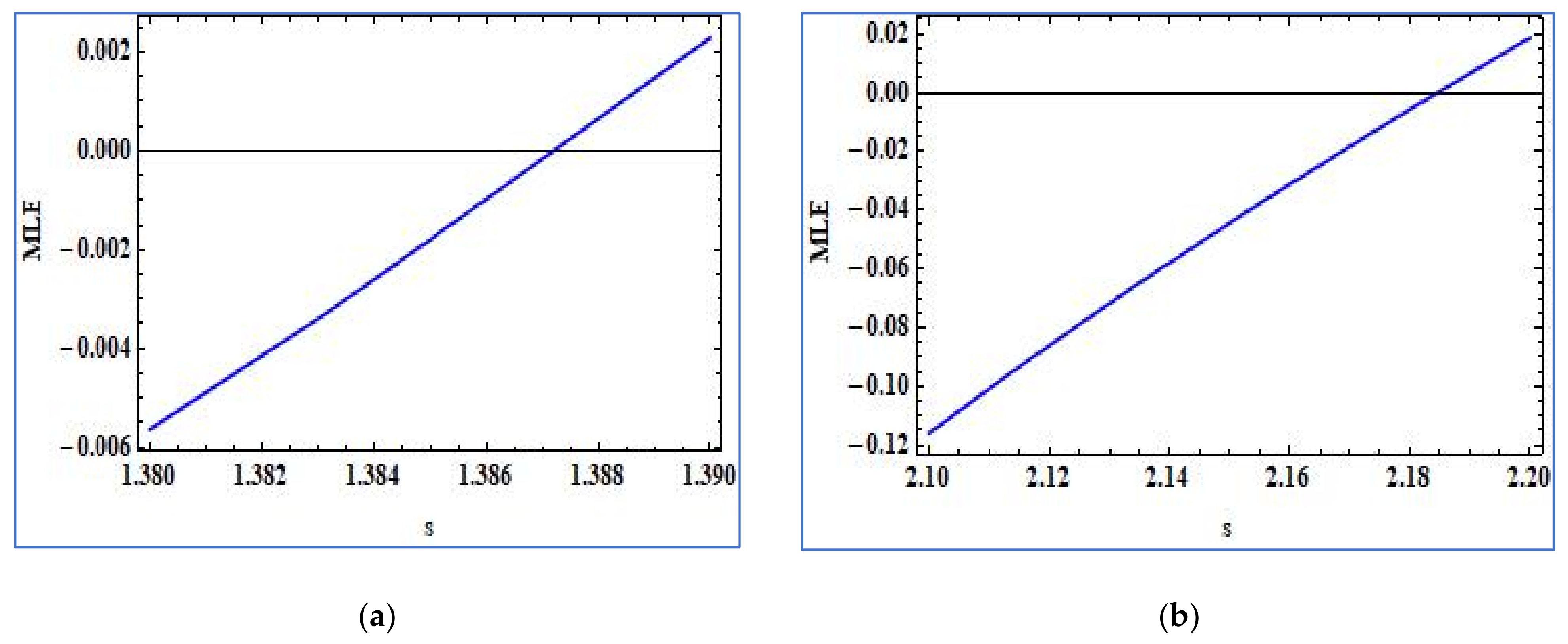
• Our findings indicate that model (4) undergoes periodic doubling as well as a Neimark-Sacker bifurcation at its unique positive equilibrium.
• The direction and existance criteria for both types of bifurcation are examined under interior equilibrium.
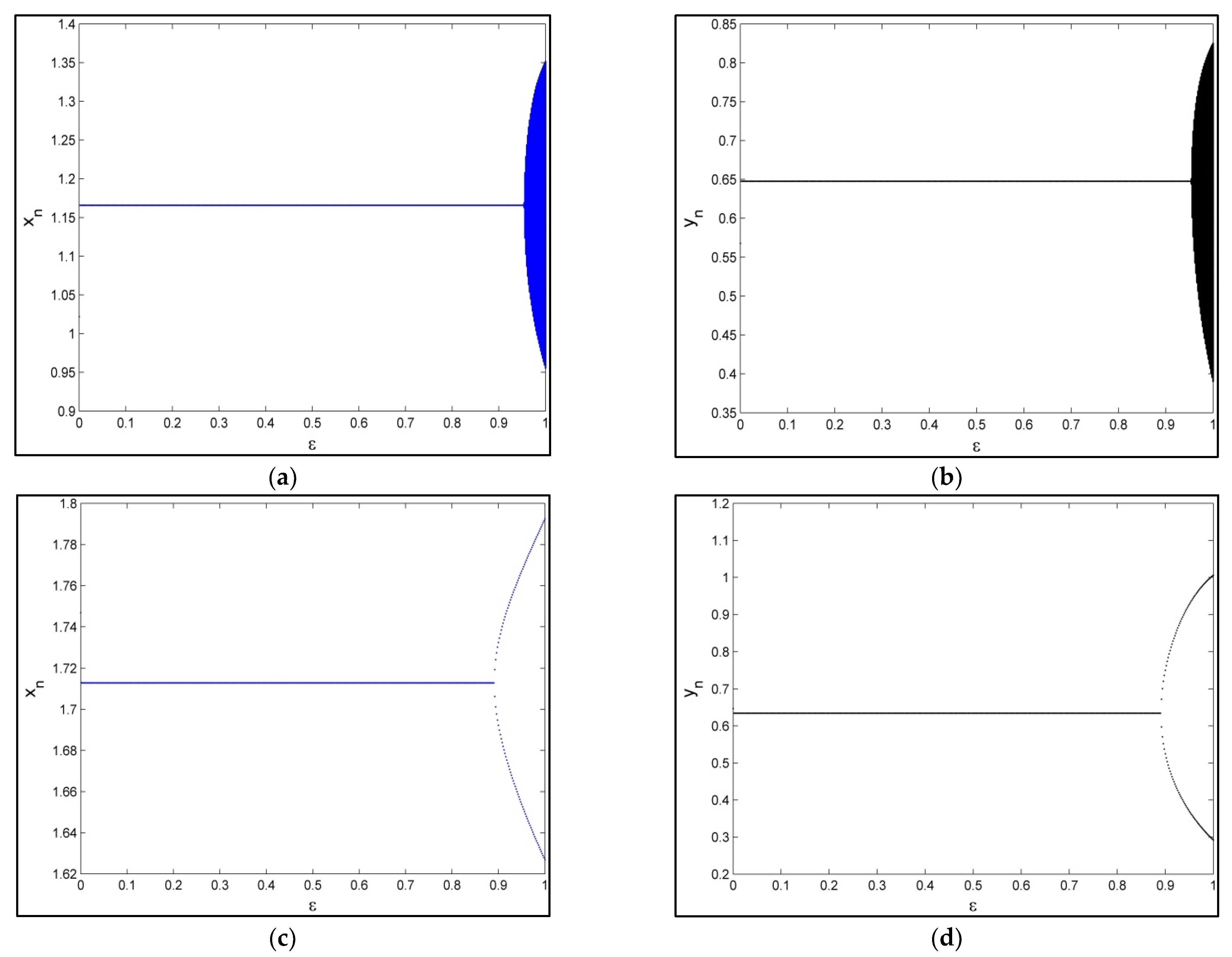
• A hybrid control strategy is applied to control the chaos in model (4).

The remainder of this paper is organized as follows. After presenting some related preliminaries in Section 2, the boundedness of the steady state is analyzed in Section 3. In Section 4, the dynamics of system (4), including the existence of equilibria and local stability, are presented. Section 5 describes an investigation of the birfurcation analysis at the interior fixed point of system (4). In Section 6, we study a hybrid control method to control the chaos. The fractal dimensions are calculated in Section 7. Finally, numerical simulations are provided in Section 8 to verify our analytical approach. Conclusions related to these results are presented in Section 9 and the future directions are providing in Section 10.

Furthermore, a detailed investigation of some charismatic population models and their qualitative behavior are provided (see, Din and Din et al. [18,19,20,21,22,23,24,25,26] and the references therein).

2. Preliminaries

Definition 1.

([32]) A point$x^{*}$is said to be a fixed point of the map for an equilibrium point if $f\left(x^{*}\right)=x^{*}$.

Theorem 1.

([32]) Let$f : I \to I$ be a continuous map, where $I=\left[a, b\right]$ is a closed interval in$R$. Then,$f$ has a fixed point.

Theorem 2.

([32]) Let$f : I=\left[a, b\right] \to R$ be a continuous map such that $f\left(I\right) \supset I$. Then, $f$ has a fixed point in$I$.

Definition 2.

([32]) Let$f : I \to I$ be a map and $x^{*}$ be a fixed point of $f$, where $I$ is an interval in the set of real numbers $R$. Then, the following conditions hold true:

• $x^{*}$is said to be stable if for any$\epsilon >0$, there exists$\delta >0$such that for all$x_0\in I$with$\left|x_0-x^{*}\right|<\delta$we have$\left|f^n\left(x_0\right)-x^{*}\right|<\epsilon$for all$n \in Z^{+}$. Otherwise, the fixed point$x^{*}$is unstable.
• $x^{*}$is said to be attractive if$\eta >0$exists, such that$\left|x_0-x^{*}\right|<\eta$implies$\underset{n\to \infty }{\lim }{f}^n\left(x_0\right)=x^{*}$.
• $x^{*}$is asymptotically stable if it is both stable and attractive. If in (2),$\eta =\infty$, then$x^{*}$is said to be globally asymptotically stable.

Definition 3.

([32]) A fixed point$x^{*}$ of a map $f$ is said to be hyperbolic if $\left|f^{\prime }\left(x^{*}\right)\right|=1$. Otherwise, it is non-hyperbolic.

Theorem 3.

([32]) Let$x^{*}$ be a hyperbolic fixed point of a map $f$, where $f$ is continuously differentiable at $x^{*}$. The following statements hold true:

• If$\left|f^{\prime }\left(x^{*}\right)\right|<1$, then$x^{*}$is asymptotically stable.
• If$\left|f^{\prime }\left(x^{*}\right)\right|>1$, then$x^{*}$is unstable.

3. Boundedness

The boundedness of system (4) is based on the following Remark.

Remark 1.

([25]) Assuming that$x_0>0$ for every $x_t$ and $x_{t+1}\le x_{t}exp\left(A\left[1-B{x}_t\right]\right)$ for every $t\in \left[t_1,\infty \right]$, where $B>0$ is constant. Then,

$$\underset{n\to \infty }{\lim }\mathrm{Sup}{x}_t\le \frac{1}{AB}\exp \left(A-1\right)$$

Using Remark 1, we state the following theorem for the uniform boundedness of system (4).

Theorem 4.

Any positive solution $\left(x_n,y_n\right)$ of model (4) is uniformly bounded.

Proof. 

Assuming that $\left(x_n,y_n\right)$ is any positive solution of system (4), we then have

$$x_{n+1}\le x_n\exp \left(r\left(1-\frac{x_n}{k}\right)\right),\mathrm{for}\mathrm{all}n=0,1,2,\dots .$$

Let $x_0>0.$ Using Remark 1, we obtain the following result.

$$\underset{n\to \infty }{\lim }\mathrm{Sup}{x}_n\le \frac{k}{r}\exp \left(r-1\right)=l_1.$$

(5)

Furthermore, from the second part of system (4), we obtain the following:

$$y_{n+1}\le y_n\exp \left(s\left(1-\frac{h{y}_n}{l_1}\right)\right).$$

Let $y_0>0.$ Applying Remark 1, we obtain the following result:

$$\underset{n\to \infty }{\lim }\mathrm{Sup}{y}_n\le \frac{l_1}{sh}\left(s-1\right)=l_2$$

(6)

Thus, it follows that ${\lim }_{n\to \infty }\mathrm{Sup}\left(x_n,y_n\right)\le l$, where $l=\max \left\{l_1,l_2\right\}$. The proof is completed. □

4. Existence of a Positive Fixed Point and Local Stability

To explore the existence of a fixed point of model (4), suppose that $\left(x,y\right)$ is any arbitrary fixed point of (4). Then, $\left(x,y\right)$ must satisfy the following algebraic system of equations:

$$\begin{array}{ll}\hfill x=& x \exp \left(r\left(1-\frac{x}{k}\right)-\frac{axy}{b^2+x^2}\right),\hfill \\ \hfill y=& y \exp \left(s\left(1-\frac{hy}{x}\right)\right).\hfill \end{array}$$

(7)

Then, (7) has a boundary equilibrium point $\left(k,0\right)$. In addition, we also explore the existence and uniqueness of the solution of system (4) because the positive fixed points are not in a closed form. For this purpose, the following computation, using Theorem 4, exhibits the existence and uniqueness of the solution to model (4).

Theorem 5.

There exists a unique positive steady-state$\left(x_{*}, y_{*}\right)\in \left[0, l_1\left]\times \right[0, l_2\right]$of system (4).

Proof. 

To attain the fixed point by solving system (7), we have

$$\begin{array}{l}r\left(1-\frac{x}{k}\right)=\frac{axy}{x^2+b^2},\hfill \\ x=yh.\hfill \end{array}$$

(8)

Suppose that

$$F\left(x\right)=r\left(1-\frac{x}{k}\right)-\frac{\frac{a{x}^2}{h}}{x^2+b^2}$$

for all $x\in \left[0, l_1\right].$ Then, we can see that $F\left(0\right)=r>0$ and

$$F\left(l_1\right)=-\frac{a\exp \left(2\left(r-1\right)\right)k^2}{h\left(b^2+\frac{\exp \left(2\left(r-1\right)\right)k^2}{r^2}\right)r^2}+r\left(1-\frac{\exp \left(r-1\right)}{r}\right)<0$$

for all $a, b, s, r, k, \mathrm{and} h>0.$ Hence, there exists at least one root of $F\left(x\right)=0$, for $x\in \left[0, l_1\right].$ In addition,

$$F\text{'}\left(x\right)=-\frac{r}{k}-\frac{2a{b}^{2}x}{h{\left(b^2+x^2\right)}^2}<0$$

for all $x\in \left[0, l_1\right].$ Therefore, the system (4) has a unique positive fixed point $\left(x_{*}, y_{*}\right)\in \left[0, l_1\left]\times \right[0, l_2\right]$.

Initially, we explored the stability analysis of the boundary equilibrium $\left(k,0\right)$. The Jacobian matrix $F_J$ evaluated at $\left(k,0\right),$ is expressed as

$$F_J\left(k,0\right)=\left[\begin{array}{cc}1-r& -\frac{k^{2}a}{b^2+k^2}\\ 0& \exp \left(\mathrm{s}\right)\end{array}\right],$$

and the characteristic equation computed at $\left(k,0\right)$ is given by

$$\mathbb{F}\left(\eta \right)={\eta }^2-\left(1-r+\exp \left(\mathrm{s}\right)\right)\eta +\left(1-r\right)\exp \left(\mathrm{s}\right)$$

Hence, $\mathbb{F}\left(\eta \right)=0$ has two roots, namely, ${\eta }_1=\exp \left(\mathrm{s}\right)$ and ${\eta }_2=1-r$. In addition, $\left(k,0\right)$ is the source if $r>2$, and is the saddle point if $0<r<2$. Next, we explored the stability analysis of the fixed points. To investigate the stability of the equilibria, we calculated the Jacobian $F_J$ of system (4) at any point $\left(x,y\right)$ as follows:

$$F_J\left(x,y\right)=\left[\begin{array}{ll}{b}_{11}\hfill & b_{12}\hfill \\ b_{21}\hfill & b_{22}\hfill \end{array}\right]$$

The characteristic polynomial of $F_J$ at $\left(x,y\right)$ is given by

$$ℝ\left(\eta \right)={\eta }^2-T_1\eta +D_1,$$

(9)

where

$$T_1=\left(b_{11}+b_{22}\right),$$

and

$$D_1=b_{11}{b}_{22}-b_{12}{b}_{21}$$

The following Lemma is extremely useful to examine the stability of the equilibria. □

Lemma 1.

Let $\Re \left(\eta \right)={\eta }^2-T_1\eta +D_1$ and $\Re \left(1\right)>0$. Moreover, ${\eta }_1$,${\eta }_2$ are the roots of equation $\Re \left(\eta \right)=0$, and thus

 (i)

$\left|{\eta }_1\right|<1$ & $\left|{\eta }_2\right|<1$ $\iff$ $\Re \left(-1\right)>0$ and $D_1<1$;

 (ii)

$\left|{\eta }_1\right|<1$ & $\left|{\eta }_2\right|>1$ or ($\left|{\eta }_1\right|>1$ and $\left|{\eta }_2\right|<1$) $\iff$ $\Re \left(-1\right)<0$;

 (iii)

$\left|{\eta }_1\right|>1$ & $\left|{\eta }_2\right|>1$ $\iff$ $\Re \left(-1\right)>0$ and $D_1>1$;

 (iv)

${\eta }_1=-1$ & $\left|{\eta }_2\right|\ne 1$ $\iff \Re \left(-1\right)=0$ and $T_1\ne 0,2$;

 (v)

${\eta }_1$and${\eta }_2$are complex and$\left|{\eta }_1\right|=1$and$\left|{\eta }_2\right|=1$ $\iff$ $T_1{}^2-4D_1<0$and$D_1=1$.

Because ${\eta }_1$ and ${\eta }_2$ are the eigenvalues of (9), the following topological results are obtained.

The equilibrium $\left(x,y\right)$ is known as a sink if $\left|{\eta }_1\right|<1$ $\mathrm{and}$ $\left|{\eta }_2\right|<1,$ which is locally asymptotically stable, and as a source if $\left|{\eta }_1\right|>1$ $\mathrm{and}$ $\left|{\eta }_2\right|>1$; thus, the nature of the source is always unstable. Moreover, the equilibrium point $\left(x,y\right)$ is always known as the saddle point if $\left|{\eta }_1\right|<1$ $\mathrm{and}$ $\left|{\eta }_2\right|>1$ or ($\left|{\eta }_1\right|>1$ $\mathrm{and}$ $\left|{\eta }_2\right|<1)$. In the case of a non-hyperbolic equilibrium $\left(x,y\right),$ either $\left|{\eta }_1\right|=1$ $\mathrm{or}$ $\left|{\eta }_2\right|=1$.

Our next aim is to discuss the local stability of the unique positive equilibrium $\left(x_{*},y_{*}\right)$ of system (4). Let (9) be the characteristic polynomial of the variational matrix evaluated at $\left(x_{*},y_{*}\right)$, such that

$$T_1=\left(2-\frac{r{x}_{*}}{k}-\mathsf{\Omega }-s)\right) \mathrm{and} D_1=\left(1-\frac{r{x}_{*}}{k}-\mathsf{\Omega }\right)\left(1-s\right)+\frac{\mathrm{s}\mathsf{\Phi }}{h}$$

where $\mathsf{\Omega }=\frac{a{x}_{*}{y}_{*}\left(b^2-x_{*}^2\right)}{{\left(b^2+x_{*}^2\right)}^2}$ and $\mathsf{\Phi }=\frac{a{x}_{*}^2}{b^2+x_{*}^2}.$ Thus, by applying Lemma 1, we discuss the local stability of system (4) around $\left(x_{*},y_{*}\right)$ by stating the following proposition.

Proposition 1.

The interior equilibrium point$\left(x_{*},y_{*}\right)$of system (4) satisfies the following results:

 (i)

The interior equilibrium$\left(x_{*},y_{*}\right)$is stable iff:

$$\left|2-\frac{r{x}_{*}}{k}-\mathsf{\Omega }-s\right|<\left|1+\left(1-\frac{r{x}_{*}}{k}-\mathsf{\Omega }\right)\left(1-s\right)+\frac{\mathrm{s}\mathsf{\Phi }}{h}\right|,$$

and

$$\left|\frac{\mathrm{s}\mathsf{\Phi }}{h}+\left(1-s\right)\left(1-\frac{r{x}_{*}}{k}-\mathsf{\Omega }\right)\right|>1$$

 (ii)

The positive fixed point$\left(x_{*},y_{*}\right)$is a saddle point if and only if

$${\left[2-\frac{r{x}_{*}}{k}-\mathsf{\Omega }-s\right]}^2>4\left[\left(1-s\right)\left(1-\frac{r{x}_{*}}{k}-\mathsf{\Omega }\right)+\frac{\mathrm{s}\mathsf{\Phi }}{h}\right],$$

and

 (iii)

The interior fixed point$\left(x_{*},y_{*}\right)$is non-hyperbolic if and only if

$$\left|2-\frac{r{x}_{*}}{k}-\mathsf{\Omega }-s\right|=\left|1+\left(1-\frac{r{x}_{*}}{k}-\mathsf{\Omega }\right)\left(1-s\right)+\frac{\mathrm{s}\mathsf{\Phi }}{h}\right|$$

(10)

or

$$\left(1-\frac{r{x}_{*}}{k}-\mathsf{\Omega }\right)\left(1-s\right)+\frac{\mathrm{s}\mathsf{\Phi }}{h}=1 and \left|2-\frac{r{x}_{*}}{k}-\mathsf{\Omega }-s\right|<2.$$

(11)

To explore the local stability criteria for $\left(x_{*},y_{*}\right)$ of model (4), we have the following theorem:

Theorem 6.

If neither (10) nor (11) is satisfied, then the positive steady-state $\left(x_{*},y_{*}\right)$of system (4) is locally asymptotically stable if and only if the following condition is satisfied.

$$\left|2-\frac{r{x}_{*}}{k}-\mathsf{\Omega }-s\right|<1+\left(1-\frac{r{x}_{*}}{k}-\mathsf{\Omega }\right)\left(1-s\right)+\frac{\mathrm{s}\mathsf{\Phi }}{h}<2$$

5. Bifurcation Analysis

In this section, we discuss the period-doubling and Neimark-Sacker bifurcations of system (4) around the interior equilibrium. Initially, we explored the period-doubling bifurcation at a positive fixed point $\left(x_{*},y_{*}\right)$ of system (4). To study the period-doubling bifurcation, assume that $T_1^2>4D_1$, that is,

$$\left(2-\frac{r{x}_{*}}{k}-\mathsf{\Omega }-s\right)>4\left[\left(1-\frac{r{x}_{*}}{k}-\mathsf{\Omega }\right)\left(1-s\right)+\frac{\mathrm{s}\mathsf{\Phi }}{h}\right]$$

(12)

and $T_1+D_1+1=0$. It then follows that

$$s:=\frac{2h\left(r{x}_{*}-\left(2-\mathsf{\Omega }\right)k\right)}{h\left(\mathsf{\Omega } k+r{x}_{*}\right)+k\left(\mathsf{\Phi }-2 h\right)}$$

(13)

Then, ${\eta }_1=-1$ and ${\eta }_2\ne 1$ if

$$\left(1-\frac{r{x}_{*}}{k}-\mathsf{\Omega }\right)\left(1-s\right)+\frac{\mathrm{s}\mathsf{\Phi }}{h}\ne \pm 1.$$

(14)

Consider the map $T_{PB}=\{\left(a,b,k,r,s\right)\in R_{+}^5$ for which (12)–(14) are thus satisfied. Then, the equilibrium $\left(x_{*},y_{*}\right)$ of system (4) sustains period-doubling bifurcation whenever the parameters deviate within the small neighborhood of $T_{PB}$. Thus, system (4) along with parameters $\left(a,b,k,r,s_1\right)\in T_{PB}$, can be written as follows:

$$\left(\begin{array}{l}x\hfill \\ y\hfill \end{array}\right)\to \left(\begin{array}{l}x{\mathrm{e}}^{r\left(1-\frac{x}{k}\right)-\frac{axy}{b^2+x^2}}\hfill \\ y{\mathrm{e}}^{s_1\left(1-\frac{hy}{x}\right)}\hfill \end{array}\right)$$

(15)

The following perturbation of system (15) can be obtained by taking $\overline{s}$ as a bifurcation parameter:

$$\left(\begin{array}{l}x\hfill \\ y\hfill \end{array}\right)\to \left(\begin{array}{l}x{\mathrm{e}}^{r\left(1-\frac{x}{k}\right)-\frac{axy}{b^2+x^2}}\hfill \\ y{\mathrm{e}}^{\left(s_1+\overline{s}\right)\left(1-\frac{hy}{x}\right)}\hfill \end{array}\right)$$

(16)

where $\left|\overline{s}\right|<<1$ denotes the least perturbation parameter. Assuming that $N=x-x_{*}, P=y-y_{*}$, system (16) is reduced to the following form:

$$\left(\begin{array}{l}N\hfill \\ P\hfill \end{array}\right)\to \left(\begin{array}{ll}{b}_{11}\hfill & b_{12}\hfill \\ b_{21}\hfill & b_{22}\hfill \end{array}\right)\left(\begin{array}{l}N\hfill \\ P\hfill \end{array}\right)+\left(\begin{array}{l}{f}_1\left(N,P,\overline{s}\right)\hfill \\ f_2\left(N,P,\overline{s}\right)\hfill \end{array}\right)$$

(17)

Here,

$$\begin{gathered} f_1\left(N,P,\overline{s}\right)=b_{13}{N}^2+b_{14}NP+b_{15}{P}^2+a_1{N}^3+a_2{N}^{2}P+a_{3}N{P}^2+a_4{P}^3 \\ +O\left({(\left|N\right|+\left|P\right|+\left|\overline{s}\right|)}^4\right), \\ {f}_2\left(N,P,\overline{s}\right)=b_{23}{N}^2+b_{24}NP+b_{25}{P}^2+d_1{N}^3+d_2{N}^{2}P+d_3{NP}^2+d_4{P}^3 \\ +c_1\overline{s}N+c_2\overline{r}P+c_3{\overline{r}}^2+c_4\overline{r}NP+c_5\overline{r}{N}^2+c_6\overline{r}{P}^2+c_7{\overline{r}}^{2}N+c_8{\overline{s}}^{2}P+c_9{\overline{r}}^3 \\ +O\left({(\left|N\right|+\left|P\right|+\left|\overline{s}\right|)}^4\right) \end{gathered}$$

Whereas the descriptions and computations of the involved coefficients are given in Appendix A.

The canonical form of (17) at $s_1=0$ can be obtained by assuming the following map:

$$\left(\begin{array}{l}N\hfill \\ P\hfill \end{array}\right)=\left(\begin{array}{ll}{b}_{12}\hfill & b_{12}\hfill \\ -1-b_{11}\hfill & {\eta }_2-b_{11}\hfill \end{array}\right)\left(\begin{array}{l}u\hfill \\ v\hfill \end{array}\right).$$

(18)

The normal form of system (17) under translation (18) can be expressed as

$$\left(\begin{array}{l}u\hfill \\ v\hfill \end{array}\right)\to \left(\begin{array}{ll}-1\hfill & 0\hfill \\ 0\hfill & {\eta }_2\hfill \end{array}\right)\left(\begin{array}{l}u\hfill \\ v\hfill \end{array}\right)+\left(\begin{array}{l}\tilde{f}\left(u,v,\overline{s}\right)\hfill \\ \tilde{g}\left(u,v,\overline{s}\right)\hfill \end{array}\right),$$

(19)

the descriptions and computations of the involved functions and parameters leading to the following expression are provided in Appendix B.

$$\begin{gathered} {\mathrm{F}}_1:={\left(\frac{{\partial }^2\tilde{f}}{\partial u\partial \overline{s}}+\frac{1}{2}\frac{\partial F}{\partial \overline{r}}\frac{{\partial }^{2}F}{\partial u^2}\right)}_{\left(0,0\right)}=\frac{c_2\left(1+b_{11}\right)}{{\eta }_2+1}-\frac{c_1{b}_{12}}{{\eta }_2+1}, \\ {\mathrm{F}}_2:={\left(\frac{1}{6}\frac{{\partial }^{3}F}{\partial u^3}+{\left(\frac{1}{2}\frac{{\partial }^{2}F}{\partial u^2}\right)}^2\right)}_{\left(0,0\right)}=t_1^2+t_5 \end{gathered}$$

Hence, we arrive at the following conclusions based on the aforementioned calculations.

Theorem 7.

There exists a period-doubling bifurcation at $\left(x_{*},y_{*}\right)$ of system (4), whenever ${\mathrm{F}}_2\ne 0$ and $r$ deviates within a small neighboring point of $s_1$. In addition, if ${\mathrm{F}}_2>0, \left({\mathrm{F}}_2<0\right),$ the orbit is period-2 stable (unstable).

Next, we investigated the Neimark-Sacker bifurcation around $\left(x_{*},y_{*}\right)$ of system (4). For identical results, we referred to the studies by Din [24,25], Shabbir et al. [20], and Jing et al. [14]. Furthermore, the equilibrium point moves around the close invariant curve, owing to the Neimark-Sacker bifurcation. To explore the Neimark-Sacker bifurcation, we find the conditions for which $\left(x_{*},y_{*}\right)$ is a non-hyperbolic point with a complex conjugate root of the characteristic equation of the unit modulus. Thus, if the following results hold true, then $\Re \left(\eta \right)=0$ has two complex conjugate roots with a unit modulus.

$$s:=\frac{\left(\mathsf{\Omega } k+r{x}_{*}\right)h}{h\left(\mathsf{\Omega } k+r{x}_{*}\right)+k\left(\mathsf{\Phi }-h\right)},$$

and

$$\left|2-\frac{r{x}_{*}}{k}-\mathsf{\Omega }-s\right|<2.$$

Consider

$$T_{NS}=\{\left(a,b,k,r,s\right)\in R_{+}^5:s=\frac{\left(\mathsf{\Omega } k+r{x}_{*}\right)h}{h\left(\mathsf{\Omega } k+r{x}_{*}\right)+k\left(\mathsf{\Phi }-h\right)} \mathrm{and} \left|2-\frac{r{x}_{*}}{k}-\mathsf{\Omega }-s\right|<2\}.$$

Assuming that $s_2=\frac{\left(\mathsf{\Omega } k+r{x}_{*}\right)h}{h\left(\mathsf{\Omega } k+r{x}_{*}\right)+k\left(\mathsf{\Phi }-h\right)}$, the fixed point $\left(x_{*},y_{*}\right)$ ensures the Neimark-Sacker bifurcation when the parameters fluctuate in the least neighborhood of $T_{NS}$. Thus, system (4) along with parameters $\left(a,b,k,r_2,s\right)$ can be expressed as follows:

$$\left(\begin{array}{l}x\hfill \\ y\hfill \end{array}\right)\to \left(\begin{array}{l}x{\mathrm{e}}^{r\left(1-\frac{x}{k}\right)-\frac{axy}{b^2+x^2}}\hfill \\ y{\mathrm{e}}^{s_2\left(1-\frac{hy}{x}\right)}\hfill \end{array}\right).$$

(20)

The following perturbation of system (20) can be obtained by taking $\tilde{s}$ as the bifurcation parameter, i.e.,

$$\left(\begin{array}{l}x\hfill \\ y\hfill \end{array}\right)\to \left(\begin{array}{l}x{\mathrm{e}}^{r\left(1-\frac{x}{k}\right)-\frac{axy}{b^2+x^2}}\hfill \\ y{\mathrm{e}}^{\left(s_2+\tilde{s}\right)\left(1-\frac{hy}{x}\right)}\hfill \end{array}\right)$$

(21)

where $\left|\tilde{s}\right|<<1$ denotes the least perturbation. Assuming that $N=x-x_{*}, P=y-y_{*}$, then system (21) takes the following modified form:

$$\left(\begin{array}{l}N\hfill \\ P\hfill \end{array}\right)\to \left(\begin{array}{ll}{a}_{11}\hfill & a_{12}\hfill \\ a_{21}\hfill & a_{22}\hfill \end{array}\right)\left(\begin{array}{l}N\hfill \\ P\hfill \end{array}\right)+\left(\begin{array}{l}{g}_1\left(N,P\right)\hfill \\ g_2\left(N,P\right)\hfill \end{array}\right),$$

(22)

where

$$\begin{gathered} g_1\left(N,P\right)=b_{13}{N}^2+b_{14}NP+b_{15}{P}^2+a_1{N}^3+a_2{N}^{2}P+a_{3}N{P}^2+a_4{P}^3 \\ +O\left({(\left|N\right|+\left|P\right|+\left|\overline{r}\right|)}^4\right), \\ {g}_2\left(N,P\right)=b_{23}{N}^2+b_{24}NP+b_{25}{P}^2+d_1{N}^3+d_2{N}^{2}P+d_3{NP}^2+d_4{P}^3 \\ +O\left({(\left|N\right|+\left|P\right|+\left|\overline{r}\right|)}^4\right). \end{gathered}$$

Here, $b_{11},b_{12}, b_{21}, b_{22},b_{13}, b_{14}, b_{15}, a_1, a_2, a_3, a_4, b_{23}, b_{24}, b_{25}, d_1, d_2, d_3,\mathrm{and} d_4,$ are defined in (17) by replacing $s_1$ by $s_2+\tilde{s}$. Let

$${\eta }^2-T_1\left(\tilde{s}\right)\eta +D_1\left(\tilde{s}\right)=0,$$

(23)

be the characteristic equation of the variational matrix of (22) evaluated at $\left(0,0\right)$, where

$$T_1\left(\tilde{s}\right)=\left(2-\frac{r{x}_{*}}{k}-\mathsf{\Omega }-\left(s_2+\tilde{s}\right)\right) \mathrm{and} D_1\left(\tilde{s}\right)=\left(1-\frac{r{x}_{*}}{k}-\mathsf{\Omega }\right)\left(1-\left(s_2+\tilde{s}\right)\right)+\frac{\left(s_2+\tilde{s}\right)\mathsf{\Phi }}{h}$$

where $\mathsf{\Omega }=\frac{a{x}_{*}{y}_{*}\left(b^2-x_{*}^2\right)}{{\left(b^2+x_{*}^2\right)}^2}$ and $\mathsf{\Phi }=\frac{a{x}_{*}^2}{b^2+x_{*}^2}.$ Because $\left(a,b,k,r,s_2\right)\in T_{NS}$, $\left|{\eta }_1\right|=\left|{\eta }_2\right|$ such that ${\eta }_1$ and ${\eta }_2$ are the complex conjugate roots of (23), it follows that

$${\eta }_1,{\eta }_2=\frac{T_1\left(\tilde{s}\right)}{2}\pm \frac{i}{2}\sqrt{4D_1\left(\tilde{s}\right)-T_1^2\left(\tilde{s}\right)}$$

We then obtain

$$\left|{\eta }_1\left|=\right|{\eta }_2\right|=\sqrt{D_1\left(\tilde{s}\right)},{\left(\frac{d\sqrt{D_1\left(\tilde{s}\right)}}{d\tilde{s}}\right)}_{\tilde{s}=0}=\frac{\left(\mathsf{\Omega } h+\mathsf{\Phi }-h\right)k+hrx}{2\sqrt{\left(\left(\mathsf{\Omega }-1\right)k+rx\right)\left(s-1\right)h+\mathsf{\Phi } ks}}\ne 0$$

Moreover, $T_1\left(0\right)=\left(2-\frac{r{x}_{*}}{k}-\mathsf{\Omega }-s_2\right)\ne 0, -1$. Because $\left(a,b,k,r,s_2\right)\in T_{NS}$, it follows that $-2<T_1\left(0\right)=\left(2-\frac{r{x}_{*}}{k}-\mathsf{\Omega }-s_2\right)<2$. Thus, we have ${\eta }_1^m,{\eta }_2^m\ne 1$ for all $m=1,2,3,4$ at $\tilde{s}=0$, for $T_1\left(0\right)\ne 0,-1,\pm 2$. Hence, for $\tilde{s}=0$, zeros of (23) do not belong to the intersection of the unit circle with coordinate axes if the following condition is satisfied:

$$2-\mathsf{\Omega }-s_2\ne \frac{r{x}_{*}}{k}, 3-\mathsf{\Omega }-s_2\ne \frac{r{x}_{*}}{k}$$

(24)

The canonical form of (22) at $\tilde{s}=0$ can be obtained by taking $\gamma =\frac{T_1\left(0\right)}{2}$, $\delta =\frac{1}{2}\sqrt{4D_1\left(0\right)-T_1^2\left(0\right)}$ and assuming

$$\left(\begin{array}{l}N\hfill \\ P\hfill \end{array}\right)=\left(\begin{array}{ll}{b}_{12}\hfill & 0\hfill \\ \gamma -b_{11}\hfill & -\delta \hfill \end{array}\right)\left(\begin{array}{l}u\hfill \\ v\hfill \end{array}\right)$$

(25)

Using transformation (25), we obtain the following canonical form of system (22):

$$\left(\begin{array}{l}u\hfill \\ v\hfill \end{array}\right)\to \left(\begin{array}{ll}\gamma \hfill & -\delta \hfill \\ \delta \hfill & \gamma \hfill \end{array}\right)\left(\begin{array}{l}u\hfill \\ v\hfill \end{array}\right)+\left(\begin{array}{l}\tilde{f}\left(u,v\right)\hfill \\ \tilde{g}\left(u,v\right)\hfill \end{array}\right)$$

(26)

where

$$\tilde{f}\left(u,v\right)=\frac{a_1{N}^3}{b_{12}}+\frac{a_2{N}^{2}P}{b_{12}}+\frac{b_{13}{N}^2}{b_{12}}+\frac{a_{3}N{P}^2}{b_{12}}+\frac{b_{14}NP}{b_{12}}+\frac{a_4{P}^3}{b_{12}}+\frac{b_{15}{P}^2}{b_{12}}+O\left({(\left|u\right|+\left|v\right|)}^4\right)$$

$$\tilde{g}\left(u,v\right)=\left(\frac{\left(\gamma -b_{11}\right)a_1}{b_{12}\delta }-\frac{d_1}{\delta }\right)N^3+\left(\frac{\left(\gamma -b_{11}\right)a_2}{b_{12}\delta }-\frac{d_2}{\delta }\right)N^{2}P$$

$$+\left(\frac{\left(\gamma -b_{11}\right)b_{13}}{b_{12}\delta }-\frac{b_{23}}{\delta }\right)N^2+\left(\frac{\left(\gamma -b_{11}\right)a_3}{b_{12}\delta }-\frac{d_3}{\delta }\right)N{P}^2$$

$$+\left(\frac{\left(\gamma -b_{11}\right)b_{14}}{b_{12}\delta }-\frac{b_{24}}{\delta }\right)NP+\left(\frac{\left(\gamma -b_{11}\right)a_4}{b_{12}\delta }-\frac{d_4}{\delta }\right)P^3$$

$$+\left(\frac{\left(\gamma -b_{11}\right)b_{15}}{b_{12}\delta }-\frac{b_{25}}{\delta }\right)P^2+O\left({(\left|u\right|+\left|v\right|)}^4\right)$$

$$N=a_{12}u \mathrm{and} <P=\left(\gamma -b_{11}\right)u-\delta v$$

Owing to the aforementioned computation, we state a nonzero real number

$$L:={\left(\left[-Re\left(\frac{\left(1-2{\eta }_1\right){\eta }_2^2}{1-{\eta }_1}{\xi }_{20}{\xi }_{11}\right)-\frac{1}{2}\left|{\xi }_{11}{|}^2-\right|{\xi }_{02}{|}^2+Re\left({\eta }_2{\xi }_{21}\right)\right]\right)}_{\tilde{c}=0}$$

where,

$${\xi }_{11}=\frac{1}{4}\left[{\tilde{f}}_{uu}+{\tilde{f}}_{vv}+i\left({\tilde{g}}_{uu}+{\tilde{g}}_{vv}\right)\right],$$

$${\xi }_{02}=\frac{1}{8}\left[{\tilde{f}}_{uu}-{\tilde{f}}_{vv}-2{\tilde{g}}_{uv}+i\left({\tilde{g}}_{uu}-{\tilde{g}}_{vv}+2{\tilde{f}}_{uv}\right)\right]$$

$${\xi }_{20}=\frac{1}{8}\left[{\tilde{f}}_{uu}-{\tilde{f}}_{vv}+2{\tilde{g}}_{uv}+i\left({\tilde{g}}_{uu}-{\tilde{g}}_{vv}-2{\tilde{f}}_{uv}\right)\right],$$

$${\xi }_{21}=\frac{1}{16}\left[{\tilde{f}}_{uuu}+{\tilde{f}}_{uvv}+{\tilde{g}}_{uuv}+{\tilde{g}}_{vvv}+i\left({\tilde{g}}_{uuu}+{\tilde{g}}_{uvv}-{\tilde{f}}_{uuv}-{\tilde{f}}_{vvv}\right)\right].$$

Ultimately, we deduced the following conclusions for the direction and existence of the Neimark-Sacker bifurcation, based on the aforementioned calculation:

Theorem 8.

There exists a Neimark-Sacker bifurcation around $\left(x_{*},y_{*}\right)$ whenever $s$ deviates wtihin the neighborhood of $s_2=\frac{\left(\mathsf{\Omega } k+r{x}_{*}\right)h}{h\left(\mathsf{\Omega } k+r{x}_{*}\right)+k\left(\mathsf{\Phi }-h\right)}$. In addition, if $L<0 (L>0)$, then an attracting (or repelling) invariant closed curve fluctuates in the range $\left(x_{*},y_{*}\right)$ for $s>s_2 (or s<s_2)$.

6. Chaos Control

In this section, we implement the hybrid control method for controlling the chaos caused by the period-doubling bifurcation and for controlling the Neimark-Sacker bifurcation in (4). Such strategies have been discussed elsewhere in [21,33,34,35,36,37]. We assume the following controlled system corresponding to model (4):

$$\begin{array}{ll}\hfill x_{n+1}=& ϵx_n\exp \left(r\left(1-\frac{x_n}{k}\right)-\frac{a{x}_n{y}_n}{b^2+x_n{}^2}\right)+\left(1-ϵ\right)x_n,\hfill \\ \hfill y_{n+1}=& ϵy_n\exp \left(s\left(1-\frac{h{y}_n}{x_n}\right)\right)+\left(1-ϵ\right)y_n,\hfill \end{array}$$

(27)

where $0<ϵ<1$. Furthermore, both types of bifurcations can be controlled by choosing an appropriate value of parameter $ϵ$. The controlled system (27) and the original system (4) have the same equilibrium point; the Jacobian matrix of the controlled system (27) at $\left(x_{*},y_{*}\right)$ is expressed by

$$\left[\begin{array}{ll}1-\frac{ϵ xr}{k}-ϵ \mathsf{\Omega }\hfill & -ϵ \mathsf{\Phi }\hfill \\ \frac{ϵ s}{h}\hfill & 1-ϵ s\hfill \end{array}\right]$$

Consequently, the necessary and sufficient condition for local stability around $\left(x_{*},y_{*}\right)$ of the controlled system (27) yields the following result.

Theorem 9.

The interior fixed point $\left(x_{*},y_{*}\right)$ of (27) is locally asymptotically stable if

$$\left|2-\frac{\epsilon r{x}_{*}}{k}-\epsilon \mathsf{\Omega }-\epsilon s\right|<1+\left(1-\frac{\epsilon r{x}_{*}}{k}-\epsilon \mathsf{\Omega }\right)\left(1-\epsilon s\right)+\frac{s\mathsf{\Phi }}{h}<2.$$

7. Fractal Dimension

The fractal dimension that describes the strange attractors of discrete-time models is defined as follows [38,39]:

$${\mathfrak{D}}_{𝓁}=𝓂+\frac{{{\displaystyle \sum }}_{j=1}^{𝓂}{𝓀}_{𝓂}}{\left|{𝓀}_{𝓂}\right|},$$

where ${𝓀}_1, {𝓀}_2,\dots ,{𝓀}_{𝓂}$ are Lyapunov exponents, and $𝓂$ is the largest integer such that ${\displaystyle \sum }_{j=1}^{𝓂}{𝓀}_{𝓂}\ge 0$ and ${\displaystyle \sum }_{j=1}^{𝓂+1}{𝓀}_{𝓂}<0.$ For the discrete-time model (4), the fractal dimension takes the following form:

$${\mathfrak{D}}_{𝓁}=1+\frac{{𝓀}_1}{\left|{𝓀}_2\right|}, {𝓀}_1>0>{𝓀}_2$$

Furthermore, for the values of parameters $a, b, r, k, h,$ and $s$, the two Lyapunov exponents ${\mathrm{F}}_1$ and ${\mathrm{F}}_2$ are computed numerically. If $b=3.3, a=0.8, r=1.3, h=2.7, \mathrm{and} k=1.8$, then ${\mathrm{F}}_1$ and ${\mathrm{F}}_2$ corresponding to the values of the bifurcation (period-doubling) parameter $s$ from the chaotic region, with the help of Mathematica software, are shown in

Table 1. Fractal dimension of model (4).

$\mathbf{Values}\mathbf{of}\mathit{s}$	$1\mathbf{st}\mathbf{Lyapunov}\mathbf{Exponents}{\mathbf{F}}_1$	$2\mathbf{nd}\mathbf{Lyapunov}\mathbf{Exponents}{\mathbf{F}}_2$	$\mathbf{Fractal}\mathbf{Dimension}{\mathfrak{D}}_{𝓁}$
2.85	$0.08462596943938297$	$-1.1368798813345231$	$1.0744370366903186$
2.90	$0.22741225178613755$	$-1.2160641186798002$	$1.187006793714976$
3.0	$0.31895100399320747$	$-1.0790255038850196$	$1.2955917194216706$
3.1	$0.22493177216760443$	$-1.244489487648406$	$1.1807422034497348$
3.2	$0.4025124673527987$	$-1.1944261491614452$	$1.3369923436751492$
3.3	$0.3894200849244259$	$-1.2328810276916689$	$1.3158618521801246$
3.4	$0.47745428811163265$	$-1.2528556268034083$	$1.3810928233844715$
3.5	$0.47582043180971084$	$-1.2925566246939908$	$1.3681234715131803$

.

The strange attractors for fixed parametric values illustrate that the discrete model (4) has a complex dynamical behavior as parameter $s$ increases by $s>2.1894756175566834$. Similarly, for the Neimark-Sacker bifurcation, the Lyapunov exponents and fractal dimension can be calculated for the values of parameter $s$ from the chaotic region, that is, $s=1.66, 1.68, 1.89,$ and so on. The strange attractors corresponding to these values are also shown in Figure 1. In particular, Figure 1g,h,k below, demonstrate that the discrete time model (4) has a complex dynamical nature when parameter $s>1.3874082082631611.$

8. Numerical Simulation

This section verifies the aforementioned theoretical discussion. The first example is related to the existence and direction of the Neimark-Sacker bifurcation. The second example shows that for a suitable choice of parameters, system (4) undergoes period-doubling bifurcation. Moreover, to confirm the control of flip and Neimark-Sacker bifurcation, we provide two examples for different choices of parameters defined in $T_{PB}$ and $T_{NS}$.

Example 1.

Let$b=1.7,a=2.26,r=2.4,h=1.8,k=1.4$, $s\in \left[1,1.8\right]$, and initial conditions$\left(x_0,y_0\right)=\left(1.0219,0.567721\right)$. Then, both species undergo a Neimark-Sacker bifurcation, as shown in Figure 2. To confirm the chaotic behavior of model (4) MLE is shown in Figure 2c.

Furthermore, Figure 1a–l shows the interesting behavior of system (4). Figure 1f–l shows the chaotic behavior of system (4). Assuming that $b=1.7$, we have a positive fixed point $\left(x_{*},y_{*}\right)=\left(1.165750001,0.6476388892\right)$, which loses stability and undergoes a Neimark-Sacker bifurcation. Thus, for the aforementioned parameters, we have the following control system:

$$\begin{array}{ll}\hfill x_{n+1}=& ϵ x_n{\mathrm{e}}^{2.4-1.714285714 x_n-2.26 \frac{x_n{y}_n}{x_n{}^2+2.89}}+\left(1-ϵ\right)x_n,\hfill \\ \hfill y_{n+1}=& ϵ y_n{\mathrm{e}}^{1.5-2.70 \frac{y_n}{x_n}}+\left(1-ϵ\right)y_n.\hfill \end{array}$$

(28)

It can be clearly observed that the controlled system (28) has a unique positive equilibrium point $\left(x_{*},y_{*}\right)=\left(1.165750001,0.6476388892\right),$ which is similar to the original system (4). In addition, the Jacobian at equilibrium $\left(x_{*},y_{*}\right)=\left(1.165750001,0.6476388892\right)$ has the following form:

$$\left[\begin{array}{ll}-2.143126283 ϵ+1\hfill & -0.7228285706 ϵ\hfill \\ 0.8333333325 ϵ\hfill & -1.500000000 ϵ+1\hfill \end{array}\right].$$

Example 2.

Assuming the parameters$b=3.3,a=0.8,r=1.3,h=2.7,k=1.8$, and$s\in \left[2,3.5\right]$, and the initial conditions$\left(x_0,y_0\right)=\left(1.74693,0.647013\right)$, both species then undergo period-doubling bifurcation when the bifurcation parameter passes through$s=2.1894756175566834,$as shown in Figure 3. In particular this fact is obvious in Figure 3a,b. Moreover, to confirm the chaotic behavior of model (4) MLE is shown in Figure 3c.

Furthermore, if $s=2.4,$ then the equilibrium point $\left(x_{*},y_{*}\right)=\left(1.712924751,0.6344165743\right)$ loses its stability and undergoes periodic doubling (see Figure 4).

Thus, for the aforementioned parameters, we present the following control system:

$$\begin{array}{ll}\hfill x_{n+1}=& ϵ x_n{\mathrm{e}}^{1.3-0.7222222223 x_n-0.8 \frac{x_n{y}_n}{x_n{}^2+10.89}}+\left(1-ϵ\right)x_n,\hfill \\ \hfill y_{n+1}=& ϵ y_n{\mathrm{e}}^{2.4-6.48 \frac{y_n}{x_n}}+\left(1-ϵ\right)y_n,\hfill \end{array}$$

(29)

The fixed point $\left(x_{*},y_{*}\right)=\left(1.712924751,0.6344165743\right)$ was preserved in the case of a controlled system (29). Furthermore, the variational matrix of the aforementioned controlled system computed at a fixed point $\left(x_{*},y_{*}\right)=\left(1.712924751,0.6344165743\right)$ is given by

$$\left[\begin{array}{ll}-1.273304693 ϵ+1\hfill & -0.1697967362 ϵ\hfill \\ 0.8888888882 ϵ\hfill & -2.399999999 ϵ+1\hfill \end{array}\right]$$

The characteristic polynomial of the aforementioned Jacobian matrix is given by

$${\eta }^2+\left(3.673304692 ϵ-2\right)\eta +3.206861694 {ϵ}^2-3.673304692 ϵ+1=0.$$

According to Lemma 1, the control system is locally asymptotically stable, if $0<ϵ<0.8910230450195268$ and bifurcation is controlled for $0<ϵ<0.8910230450195268$ (see Figure 4c,d).

Finally, some local implications of the MLE diagrams, shown in Figure 1c and Figure 2c for the Neimark-Sacker bifurcation and period-doubling bifurcation, respectively, are plotted in Figure 5a,b, respectively. It has also been verified that the system undergoes Neimark-Sacker bifurcation at $s=1.3874082082631611$, where the phase portrait at this point shows a closed invariant curve, as already shown in Figure 4c.

9. Concluding Remarks

In this study, we examined the qualitative and dynamical analyses of a discrete-time predator-prey model. Piecewise constant arguments have been applied to achieve the discrete-time counterpart of a continuous model. Thus, a comprehensive analysis of model (4) was presented. In particular, we investigated the boundedness, local stability of the boundary, and positive equilibrium points, which seem to present more challenging cases of Euler’s discretization scheme in [31]. Moreover, it was proved that the population sustains both period-doubling bifurcation and Neimark-Sacker bifurcation near the interior equilibrium. The parametric conditions were obtained for the direction and existence of both types of bifurcations using the theory of bifurcation and center manifold theorem. Moreover, the chaotic attractors shown in Figure 5 ensures chaos in the system. To control the chaotic behavior of system (4), a hybrid control method was implemented. Hence, by applying a control strategy, both types of bifurcations can be controlled for a maximum range of control parameters. We also presented the fractal dimension of model (4), which characterizes the strange attractors provided in Figure 5 thereby illustrating the complexity and rich dynamics of discrete model (4). Finally, numerical simulations were conducted to verify the analytical and theoretical approaches.

10. Future Direction

Our future research will include the Leslie–Gower predator-prey model with the functional response of Holling type-II. In this case, we aim to conduct stability, bifurcation, and chaos-control analyses of the model. A comparison of both functional responses will be conducted in a future study.

References

1. Chen, B.S.; Chen, J.J. Bifurcation and chaotic behavior of a discrete singular biological economic system. Appl. Math. Comput. 2012, 219, 2371–2386. [Google Scholar] [CrossRef]
2. Ghaziani, R.K.; Govaerts, W.; Sonck, C. Resonance and bifurcation in a discrete-time predator-prey system with Holling functional response. Nonlinear Anal. RWA 2012, 13, 1451–1465. [Google Scholar] [CrossRef] [Green Version]
3. Jana, D. Chaotic dynamics of a discrete predator-prey system with prey refuge. Appl. Math. Comput. 2013, 224, 848–865. [Google Scholar] [CrossRef]
4. Misra, O.P.; Sinha, P.; Singh, C. Stability and bifurcation analysis of a prey-predator model with age based predation. Appl. Math. Model. 2013, 37, 6519–6529. [Google Scholar] [CrossRef]
5. Zhang, G.D.; Shen, Y.; Chen, B.S. Bifurcation analysis in a discrete differential-algebraic predator-prey system. Appl. Math. Model. 2014, 38, 4835–4848. [Google Scholar] [CrossRef]
6. Hu, D.P.; Cao, H.J. Bifurcation and chaos in a discrete-time predator-prey system of Holling and Leslie type. Commun. Nonlinear Sci. Numer. Simulat. 2015, 22, 702–715. [Google Scholar] [CrossRef]
7. Wang, C.; Li, X.Y. Further investigations into the stability and bifurcation of a discrete predator-prey model. J. Math. Anal. Appl. 2015, 422, 920–939. [Google Scholar] [CrossRef]
8. Murdoch, W.; Briggs, C.; Nisbet, R. Consumer-Resource Dynamics; Princeton University Press: New York, NY, USA, 2003. [Google Scholar]
9. Holling, C.S. The functional response of predator to prey density and its role in mimicry and population regulation. Mem. Entomol. Soc. Can. 1965, 97, 5–60. [Google Scholar] [CrossRef] [Green Version]
10. Rosenzweig, M.L.; MacArthur, R.H. Graphical representation and stability conditions of predator-prey interactions. Am. Nat. 1963, 97, 209–223. [Google Scholar] [CrossRef]
11. Freedman, H.I.; Mathsen, R.M. Persistence in predator-prey systems with ratio-dependent predator influence. Bull. Math. Biol. 1993, 55, 817–827. [Google Scholar] [CrossRef]
12. Hastings, A. Multiple limit cycles in predator-prey models. J. Math. Biol. 1981, 11, 51–63. [Google Scholar] [CrossRef]
13. Lindstrom, T. Qualitative analysis of a predator-prey systems with limit cycles. J. Math. Biol. 1993, 31, 541–561. [Google Scholar] [CrossRef]
14. Jing, Z.J.; Yang, J. Bifurcation and chaos in discrete-time predator-prey system. Chaos Solitons Fractals 2006, 27, 259–277. [Google Scholar] [CrossRef]
15. Liu, X.; Xiao, D. Complex dynamic behaviors of a discrete-time predator-prey system. Chaos Solitons Fractals 2007, 32, 80–94. [Google Scholar] [CrossRef]
16. Lopez-Ruiz, R.; Fournier-Prunaret, D. Indirect Allee effect, bistability and chaotic oscillations in a predator-prey discrete model of logistic type. Chaos Solitons Fractals 2005, 24, 85–101. [Google Scholar] [CrossRef]
17. Neubert, M.G.; Kot, M. The subcritical collapse of predator populations in discrete-time predator-prey models. Math. Biosci. 1992, 110, 45–66. [Google Scholar] [CrossRef]
18. Shabbir, M.S.; Din, Q.; Ahmad, K.; Tassaddiq, A.; Soori, A.H.; Khan, M.A. Stability, bifurcation and chaos control of a novel discrete-time model involving Allee effect and cannibalism. Adv. Differ. Equ. 2020, 2020, 379. [Google Scholar] [CrossRef]
19. Din, Q.; Shabbir, M.S.; Khan, M.A.; Ahmad, K. Bifurcation analysis and chaos control for a plant-herbivore model with weak predator functional response. J. Biol. Dyn. 2019, 13, 481–501. [Google Scholar] [CrossRef] [Green Version]
20. Shabbir, M.S.; Din, Q.; Safeer, M.; Khan, M.A.; Ahmad, K.A. A dynamically consistent nonstandard finite difference scheme for a predator-prey model. Adv. Differ. Equ. 2019, 2019, 381. [Google Scholar] [CrossRef] [Green Version]
21. Samaddar, S.; Dhar, M.; Bhattacharya, P. Effect of fear on prey-predator dynamics: Exploring the role of prey refuge and additional food. Chaos Interdiscip. J. Nonlinear Sci. 2020, 30, 63129. [Google Scholar] [CrossRef]
22. Anacleto, M.; Vidal, C. Dynamics of a delayed predator-prey model with Allee effect and Holling type II functional response. Math. Methods Appl. Sci. 2020, 43, 5708–5728. [Google Scholar] [CrossRef]
23. Tang, B. Dynamics for a fractional-order predator-prey model with group defense. Sci. Rep. 2020, 10, 4906. [Google Scholar] [CrossRef]
24. Sarwardi, S.; Haque, M.M.; Hossain, S. Analysis of Bogdanov-Takens bifurcations in a spatiotemporal harvested-predator and prey system with Beddington–DeAngelis-type response function. Nonlinear Dyn. 2020, 100, 1755–1778. [Google Scholar] [CrossRef]
25. Din, Q. Complexity and chaos control in a discrete-time prey-predator model. Commun. Nonlinear. Sci. Numer. Simulat. 2017, 49, 113–134. [Google Scholar] [CrossRef]
26. Shabbir, M.S.; Din, Q.; Alabdan, R.; Tassaddiq, A.; Ahmad, K. Dynamical complexity in a class of novel discrete-time predator-prey interaction with cannibalism. IEEE Access 2020, 8, 100226–100240. [Google Scholar] [CrossRef]
27. Selvam, A.G.; Vianny, D.A.; Jacob, S.B. Dynamical behaviour of discrete time prey-predator model with Holling type III functional response. Cikitusi J. Multidiscip. Res. 2019, 6, 75–81. [Google Scholar]
28. Jiangang, Z.; Tian, D.; Yandong, C.; Shuang, Q.; Wenju, D.; Hongwei, L. Stability and bifurcation analysis of a discrete predator-prey model with Holling type III functional response. J. Nonlinear Sci. Appl. 2016, 2016, 6228–6243. [Google Scholar]
29. Elettreby, M.F.; Nabil, T.; Khawagi, A. Stability and bifurcation analysis of a discrete predator-prey model with mixed Holling interaction. Comput. Modeling Eng. Sci. 2020, 122, 907–921. [Google Scholar] [CrossRef]
30. Murray, J.D. Mathematical Biology, 2nd ed.; Springer: Berlin, Germany, 1993. [Google Scholar]
31. He, Z.; Lai, X. Bifurcation and chaotic behavior of a discrete-time predator-prey system. Nonlinear Anal. Real World Appl. 2011, 12, 403–417. [Google Scholar] [CrossRef]
32. Saber, N. Elaydi, Discrete Chaos; Chapman & Hall/CRC: Boca Raton, FL, USA, 2007. [Google Scholar]
33. Chen, Y.U. Controlling and anti-controlling Hopf bifurcations in discrete maps using polynomial functions. Chaos Solitons Fractals 2005, 26, 1231–1248. [Google Scholar] [CrossRef]
34. ELabbasy, E.M.; Agiza, H.N.; Metwally, H.E.L.; Elsadany, A.A. Bifurcation analysis, chaos and control in the Burgers mapping. Int. J. Nonlinear Sci. 2007, 4, 171–185. [Google Scholar]
35. Tassaddiq, A.; Shabbir, M.S.; Din, Q.; Ahmad, K. A ratio-dependent nonlinear predator-prey model with certain dynamical results. IEEE Access 2020, 8, 195074–195088. [Google Scholar] [CrossRef]
36. Din, Q.; Saleem, N.; Shabbir, M.S. A class of discrete predator-prey interaction with bifurcation analysis and chaos control. Math. Model. Nat. Phenom. 2020, 15, 1–27. [Google Scholar] [CrossRef]
37. Din, Q.; Shabbir, M.S. A Cubic autocatalator chemical reaction model with limit cycle analysis and consistency preserving discretization. MATCH Commun. Math. Comput. Chem. 2022, 87, 441–462. [Google Scholar] [CrossRef]
38. Cartwright, J.H.E. Nonlinear stiffness Lyapunov exponents and attractor dimension. Phys. Lett. A 1999, 264, 298–304. [Google Scholar] [CrossRef] [Green Version]
39. Kaplan, J.L.; Yorke, J.A. Preturbulence: A regime observed in a fluid flow model of Lorenz. Commun. Math. Phys. 1979, 67, 93–108. [Google Scholar] [CrossRef]
Figure 1. a   s = 1.34 , b   s = 1.3811 ,   c   s = 1.3874082082631611 , d   s = 1.43 , e   s = 1.607 , f   s = 1.625 , g   s = 1.66 ,   h   s = 1.68 , i   s = 1.735 , j   s = 1.83 , k   s = 1.89 , l   s = 1.99 . (a)–(l) Phase portraits of system (4) for different values of s 1 , 2 with b = 1.7 , a = 2.26 , r = 2.4 , h = 1.8 , and   k = 1.4 under the initial conditions x 0 = 1.0219 , y 0 = 0.567721 .
Fractalfract 06 00031 g001aFractalfract 06 00031 g001b
Figure 2. Bifurcation diagrams and maximum Lypunov exponents (MLE) for system (4) with parametric values b = 1.7 ,   a = 2.26 ,   r = 2.4 ,   h = 1.8 ,   k = 1.4 , and s 1 , 1.8 and initial conditions x 0 , y 0 = 1.0219 , 0.567721 : (a) bifurcation for x n , (b) bifurcation for y n , and (c) MLE.
Fractalfract 06 00031 g002
Figure 3. Bifurcation diagrams and MLE for system (4) with parameters b = 3.3 ,   a = 0.8 ,   r = 1.3 ,   h = 2.7 ,   k = 1.8 , s 2 ,   3 , and x 0 , y 0 = 1.74693 , 0.647013 : (a) period-doubling bifurcation for x n , (b) period-doubling bifurcation for y n , and (c) MLE.
Fractalfract 06 00031 g003
Figure 4. (a) Bifurcation diagrams of x n for controlled system (28), (b) bifurcation diagrams of y n for controlled system (28), (c) bifurcation diagrams of x n for controlled system (30), and (d) bifurcation diagrams of y n for controlled system (30).
Fractalfract 06 00031 g004
Figure 5. (a) Local implication for the Neimark-Sacker bifurcation and (b) local implication for period-doubling bifurcation.
Fractalfract 06 00031 g005