Abstract
In this work, we present a modified generalized Mittag–Leffler function method (MGMLFM) and Laplace Adomian decomposition method (LADM) to get an analytic-approximate solution for nonlinear systems of partial differential equations (PDEs) of fractional-order in the Caputo derivative. We apply the MGMLFM and LADM on systems of nonlinear time-fractional PDEs. Precisely, we consider some important fractional-order nonlinear systems, namely Broer–Kaup (BK) and Burgers, which have found major significance because they arise in many physical applications such as shock wave, wave processes, vorticity transport, dispersal in porous media, and hydrodynamic turbulence. The analysis of these methods is implemented on the BK, Burgers systems and solutions have been offered in a simple formula. We show our results in figures and tables to demonstrate the efficiency and reliability of the used methods. Furthermore, our outcome converges rapidly to the given exact solutions.
1. Introduction
Mathematical models within fractional calculus (FC) have been widely used in various fields of natural science and engineering. In the last few decades, throughout much of the literature, we can find the concept of “memory” as the main advantage to process a system of fractional differential equations. This property has a significant impact on the behavior of the solutions for the considered models (see, e.g., [1,2]). The non-locality property of the fractional derivatives [3,4] that gives preference to utilizing FC, means calculating a time-fractional derivative of a function at some time and requires all the previous history. This effect justifies the use of FC to better explain real-life models. In general, these models actually made more progress than those without the memory concept [5,6,7]. Recently, some authors have added a significant amount of research in the area of FC and its applications in various branches of engineering and natural science, such as electrodynamics [8], nano-technology [9], finance [10], mathematical biology [11,12], and control theory [13,14].
There are numerous phenomena in physics, biology, chemistry, engineering, finance, and other applied sciences that are represented by differential equations. In recent years, there have been a special interest in fractional partial differential equations (FPDEs), especially nonlinear ones, because of their influence in many applied sciences, such as diffusion of biological populations, fluid flow, electromagnetic waves, control theory of dynamical systems, and so on (see, e.g., [15,16,17,18,19] and the references therein). The majority of scientific problems in physics, engineering, and biological systems are nonlinear and their exact solutions are not easy to find. For example, physical problems are mostly modeled using higher nonlinear FPDEs. In fact, it is challenging to find the exact solutions to such problems. Consequently, numerical and approximate techniques must be applied. Many useful approaches have been utilized to solve nonlinear and linear fractional differential equations (FDEs), such as the Adomian decomposition method (ADM) [20], variational iteration method (VIM) [21,22], homotopy analysis method (HAM) [23,24,25,26], homotopy perturbation method (HPM) [27,28,29].
The Mittag–Leffler function (MLF) has acquired major significance because its participation in solving numerous applications of FDEs. The generalized MLF method (GMLFM) is utilized to solve ordinary FDEs [30]. The GMLFM is applied to find analytical and approximate solutions for nonlinear systems that have applications such as the smoking model [31,32], Lorenz system [33], Riccati differential equations [34], and so on. The efficiency and eligibility of the GMLFM derive from the fact that its results converge promptly to the exact solution, and that it also provides solutions in simple and convenient procedures. Moreover, the GMLFM can be modified to solve FPDES, where the MLF undetermined coefficient method contributes to solve the homogeneous FPDEs [35]. The modification of the GMLFM was applied to solve time-fractional Korteweg–de Vries (KdV) and Korteweg–de Vries–Burgers (KdVB) equations [36]. Furthermore, this modification has been used to illustrate the dynamics of predator–prey population as in [37].
The Adomian decomposition method (ADM) is an effective analytical method, that was first introduced by Adomian in the 1980s (see, e.g., [38,39]) to solve differential equations describing physical phenomena [40]. Furthermore, the ADM was developed by using Laplace transformation. Briefly, the LADM has been developed using the Laplace transform and ADM. Thus, we can say that the LADM demonstrates how the Laplace transform may be combined with the ADM to obtain an analytic approximate solution of nonlinear differential equations. Precisely, we used the LDAM because the calculations are easy to follow and understand. Additionally, the LADM is able to converge to the exact solutions faster than the ADM. For more advantages of the LADM over ADM and the comparison between them, see, e.g., [41]. Numerous phenomena that are described by PDE and FPDEs have been solved using the LADM, like Swift–Hohenberg (SH) equation [42], Keller–Segel equation [43], time-fractional model of Navier–Stokes equation [44], Fisher’s equation [45], fractional-order telegraph equations [46], and third-order dispersive FPDEs [47].
In this article, we intend to obtain the analytical solution of the following nonlinear fractional partial differential equations (NFPDEs):
- Broer–Kaup (BK) sytem [48] of fractional orderwith the initial conditions (ICs)
- Burgers’ system [49] of fractional orderwith the ICs
- Burgers’ system [49]:with the ICs
The motivation of this study was to introduce two analytical techniques called MGMLFM and LADM to solve a full general NFPDE. In order to determine the efficacy and accuracy of the used methods, we applied them to solve the previous nonlinear systems of FPDEs and compared the obtained results with known exact solutions and solutions obtained by other methods. Precisely, to the best knowledge of the authors, analytical solutions of Broer–Kaup and Burgers’ systems of fractional orders by the proposed methods have not previously been reported in the literature, which strongly motivated this work.
The rest of this article is structured as: Section 2, we present some necessary concepts of FC, helping us to understand the main results in this article. In Section 3, we introduce the analysis of the proposed methods to solve a general system of FPDEs. Section 4 is devoted to applying the MGMLFM and LADM to the construction of approximate solutions of some illustrative examples of nonlinear systems of FPDEs. Moreover, we offer numerical simulations to compare our results with the exact solution, in order to prove the accuracy and efficacy of our methodology. Finally, our conclusion is presented in Section 5.
2. Preliminaries
In this section, we give a brief overview of the most important definitions and concepts related to this article (see, e.g., [50,51,52]).
Definition 1.
The Riemann–Liouville fractional integral of order of a function can be defined as
where is the Euler gamma function, defined as follows:
Definition 2.
The Caputo fractional partial derivative of a function of order α is defined as
for In particular, for the Caputo fractional partial derivative becomes
Theorem 1.
Let be a differentiable function in the interval , . Then,
Proposition 1.
For and , we have:
Definition 3.
Let be the Laplace transform of the function . Then, the Laplace transform of the Caputo fractional partial derivative is given by [53]
Definition 4.
The two-parameter MLF is defined by:
If , this function is denoted by and if this function represents .
Lemma 1.
The fractional derivative of the GMLF is given as:
Theorem 2.
Assume that a nonlinear function and then (see, e.g., [54])
3. Idea of the Used Methods
In this section, we introduce the idea behind the analysis of the proposed methods and how these methods were implemented to solve a general form of NFPDEs. For more details on the convergence analysis of these methods, we encourage the reader to consult [30,31,32,33,55].
3.1. Analysis of the MGMLFM
In this subsection, we discuss the methodology of the MGMLFM to solve a general FPDEs. To this end, we consider a system of fractional-order nonlinear PDEs of the following general form
with the ICs
where is the Caputo fractional derivative of order for the function , such that , and The nonlinear and linear operator of the function are represented by L and N, respectively.
The MGMLFM assumes that the solution of in Equation (7) can be written as an infinite series as follows:
where are undetermined coefficients and are functions of the variable By using ICs (8), we have
Therefore, the linear term can be decomposed as
where is a constant. From He’s polynomials [54,56,57] and Theorem 2, the can be decomposed as:
3.2. LADM for System of FDEs
Here, we explain the basic idea of the LADM for solving Equations (7) and (8). By applying the Laplace transform to both sides of Equation (7) and using the linear property of this transformation, the result is
Using Definition 3 and applying the formulas of the Laplace transform, we get:
The LADM represents the solution as an infinite series
and the nonlinear terms in Equation (7) decompose as
where are Adomian polynomials and they can be calculated by the following formula:
Then, we can write:
Then, applying the inverse Laplace transform to Equation (17), we obtain the values recursively.
4. Applications and Results
Here, we apply the MGMLFM and LADM on Equations (1), (3), and (5) and provide a comparison of the obtained results with the given exact solutions to present the accuracy and advantages of the used approaches.
Example 1.
- where are coefficients. From ICs (2), we have and By using Equation (11), we write the linear term of (1) as follows:Similarly, the nonlinear term of Equation (1) is given aswhereThen, the RR are given bySubstituting the values of n and doing some computation, we obtain the following:
- To implement the LADM, we take the Laplace transform of Equation (1); then,and by using the differential property of the Laplace transform, we have:As in the LADM, the solution can be represented as an infinite seriesand the nonlinear term in Equation (1) can be decomposed aswhere and are Adomian polynomials, which can be calculated by the following formulas:By applying the inverse Laplace transform on both sides of Equation (25), we obtainwhereThe nonlinear terms and can be written as:In order to obtain the other terms of the projected solutions, we substitute the values of Equations (27) and (28) into Equation (26), yielding:Finally, we approximate the analytic solution and by
In Table 1 and Table 2, the MGMLFM approximate solutions of Example 1 are shown for various values of α and compared with the exact solution. The tabled results below seem to coincide with the values of the exact solution (18), which means that the MGMLFM is a more accurate technique than those methods that give a solution as an infinite series.

Table 1.
Values of approximate solutions obtained by the MGMLFM, exact solution, and absolute errors of for system (1) with various values of and x.

Table 2.
Values of approximate solutions obtained by the MGMLFM, exact solution, and absolute errors of for system (1) with various values of and x.
In Figure 1 and Figure 2 the LADM approximate solutions of and at various values of α are plotted in the domain ; Moreover, a 3D graph with comparative results at is shown.
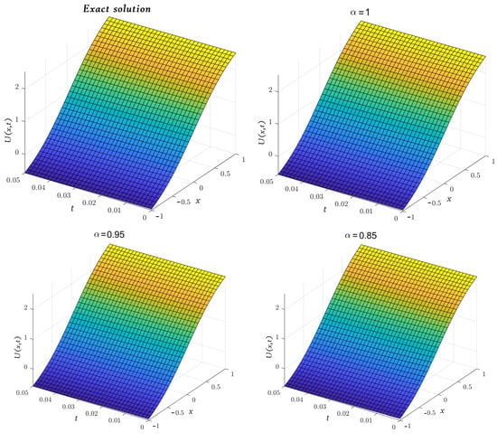
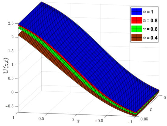
Figure 1.
Three-dimensional plots of the approximate and exact solutions of (Example 1) using the LADM.
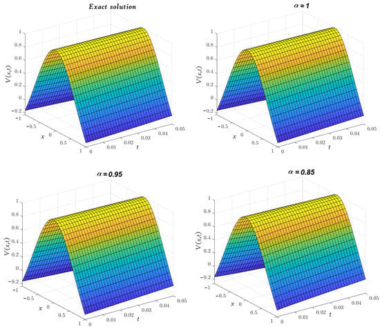
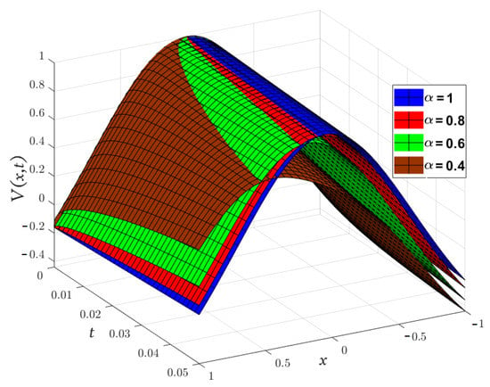
Figure 2.
Three-dimensional plots of the approximate and exact solutions of (Example 2) using the LADM.
Figure 3 represents the 2D graphs of the exact solution and the LADM solutions of and for , and .
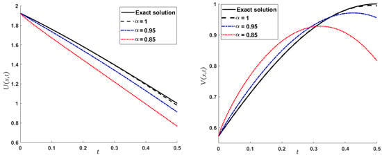
Figure 3.
Two-dimensional plots of the approximate and exact solutions of (Example 2) using the LADM, when (right figure) and (left figure).
Example 2.
- From ICs (4), we have and By using Equation (11), we obtain the linear term of Equation (3) as follows:Similarly, the nonlinear term of Equation (3) can be written as:Then, the RR are given by:By substituting values of n, we have:
- To implement the LADM, we take the Laplace transform of both sides of Equation (3); then,using the properties of the Laplace transform, we obtain:The next step in the LADM is to represent the solution as Equation (23), and the nonlinear terms and are decomposed aswhere and are Adomian polynomials and their components are defined as:Applying the inverse Laplace transform on both sides of Equation (33), we getwhereFor the other terms, we can write:Finally, we approximate the analytic solution and by
Obviously, the results in Table 3 are very close to the exact solution shown earlier in Equation (29) when which means that the approximate solutions obtained by the MGMLFM are rapidly converging to the exact solutions. Now, the LADM solutions for system (3) with ICs (4) are illustrated by the following simulation.

Table 3.
Values of approximate solutions obtained by MGMLFM, FNDM, exact solution, and absolute errors of and for system (3) with various values of and .
In Figure 4, we compare the obtained solutions by the LADM for and with the exact solution (29). Moreover, this figure illustrates the results obtained by the LADM for and with .
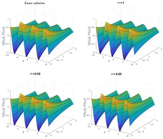
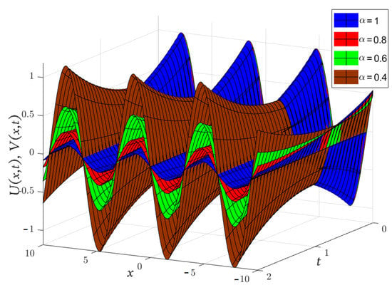
Figure 4.
Three-dimensional plots of the approximate and exact solutions of (Example 3) using the LADM.
Further, in Figure 5, we display the comparison between exact and approximate solutions in two dimensions with time (right figure) and with various values of space (left figure). Finally, it is noticeable that the LADM and MGMLFM approximate solutions overlap (for any interval of the variables ) and have a high degree of accuracy when compared to the exact solution.
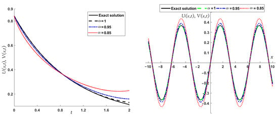
Figure 5.
Two-dimensional plots of the approximate and exact solutions of (Example 2) using the LADM, when (right figure) and t = 1 (left figure).
Example 3.
- To apply the MGMLFM, we assumewhere , and S are undetermined coefficients. From ICs (6), we have and Similarly, as in Example 2, we calculate the linear and nonlinear parts of the system (5) and using Equation (10), we getwhere and Then, the RR are given byBy substituting different values of n and using Equation (36) we get the approximate solutions in the following:
- To implement the LADM, we take the Laplace transform of Equation (5),using the Laplace transform of the Caputo derivative, we haveRepresenting the solution , and as an infinite series, as follows,the nonlinear terms included in Equation (5) can be decomposed aswhere and are Adomian polynomials defined as:by apply the inverse Laplace transform to Equation (40), we getwhereThen, it follows that for the remaining terms we obtain the solutionThe other terms of and can be computed, respectively, in the same way and according to the ADM the solution is as follows:
The results in Table 4, Table 5 and Table 6 coincide with the exact solutions described in Equation (35) when . This confirms that the approximate solutions obtained by the MGMLFM are rapidly converging to the exact solutions and this is explained in the following tables.

Table 4.
Values of approximate solutions obtained by MGMLFM, FNDM, exact solution, and absolute errors of U for system (5) with various values of and .

Table 5.
Values of approximate solutions obtained by MGMLFM, FNDM, exact solution, and absolute errors of V for system (5) with various values of and .

Table 6.
Values of approximate solutions obtained by MGMLFM, FNDM, exact solution, and absolute errors of W for system (5) with various values of and .
In Figure 6, Figure 7, Figure 8, we compare the approximate solution obtained by the LADM for , , and with the exact solution. Furthermore, Figure 9
represents the solutions obtained by the LADM for , , and with various values of α, and .
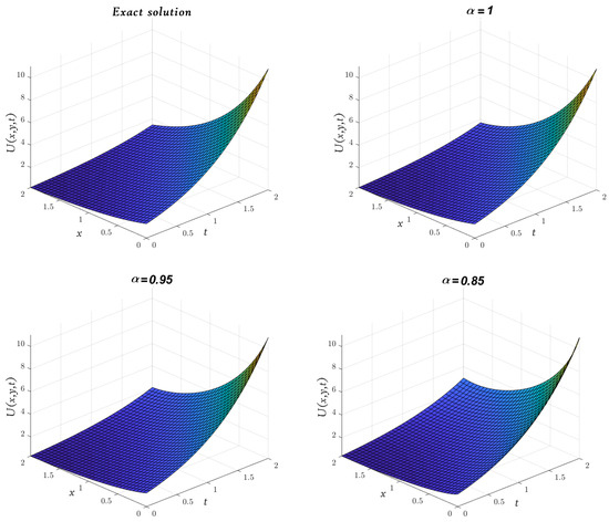
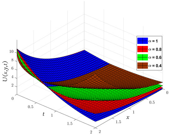
Figure 6.
Three-dimensional plots of the approximate and exact solutions of (Example 3) using the LADM.
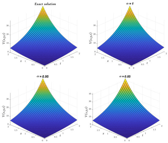
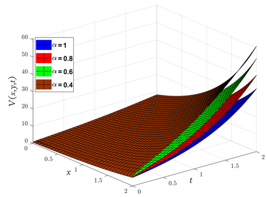
Figure 7.
Three-dimensional plots of the approximate and exact solutions of (Example 3) using the LADM.
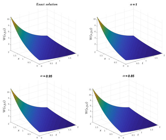
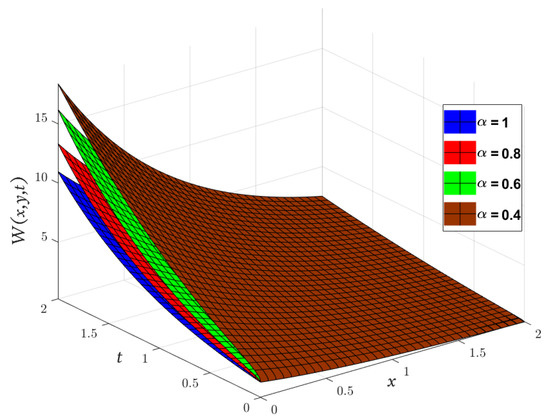
Figure 8.
Three-dimensional plots of the approximate and exact solutions of (Example 3) using the LADM.
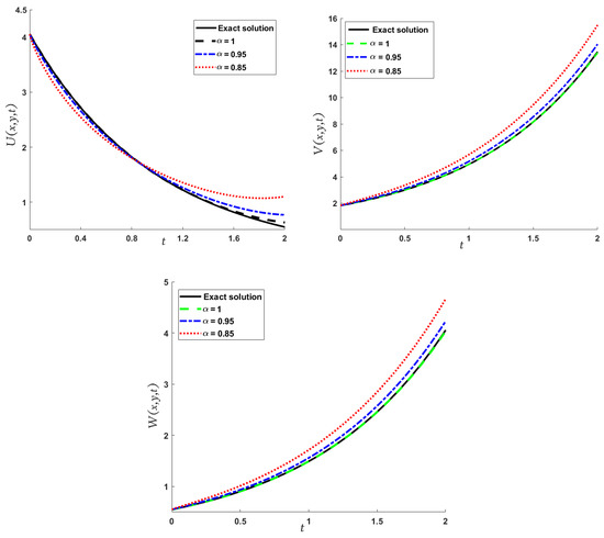
Figure 9.
Two-dimensional plots of the approximate and exact solutions of (Example 3) using the LADM, when and .
5. Conclusions
In this article, the MGMLFM and LADM were successfully used to find analytic-approximate solutions for the NFPDEs. Moreover, we focused on solving fractional-order Broer–Kaup and Burgers’ systems that arise in many physical applications, and displayed our contributions in tables and figures for different domains of . The LADM and MGMLFM solutions were presented at different values of and also for classical case (i.e., ), which showed a highly coincide with the exact solutions for all considered problems. The analysis and computations confirmed that the approximate solutions offered by the MGMLFM and LADM had rapid convergence, required low computational cost, and provided highly accurate results compared to other analytical methods. Briefly, the obtained results together with their graphical simulations revealed the complete efficiency and accuracy of the proposed methods.
Our results motivate us to deal with other types of NFPDEs. For example, in the future, the used methods can be implemented to get the analytic-approximate solution for systems of NFPDEs that arise widely in the mathematical formulation of epidemiological models for different populations.
Author Contributions
Conceptualization, H.M.A. and I.G.A.; formal analysis, I.G.A., S.A. and H.M.A.; investigation, H.M.A. and I.G.A.; methodology, H.M.A. and I.G.A.; resources, I.G.A. and H.M.A.; software, I.G.A. and H.M.A.; validation, H.M.A. and I.G.A.; visualization, H.M.A. and I.G.A.; writing—original draft, I.G.A. and H.M.A.; writing—review and editing, H.M.A., H.A. and I.G.A.; writing-revised draft, S.A.; data curation, H.A.; project administration, H.A.; funding acquisition, S.A.; All authors have read and agreed to the published version of the manuscript.
Funding
This research received no external funding.
Data Availability Statement
Data can be provided on request.
Acknowledgments
Research Supporting Project number (RSP-2021/167), King Saud University, Riyadh, Saudi Arabia.
Conflicts of Interest
The authors declare no conflict of interest regarding the publication of this paper.
References
- Tarasov, V.E. Non-Linear Macroeconomic Models of Growth with Memory. Mathematics 2020, 8, 2078. [Google Scholar] [CrossRef]
- Sardar, T.; Rana, S.; Bhattacharya, S.; Al-Khaled, K.; Chattopadhyay, J. A generic model for a single strain mosquito-transmitted disease with memory on the host and the vector. Math. Biosci. 2015, 263, 18–36. [Google Scholar] [CrossRef] [PubMed]
- Tarasov, V.E. No nonlocality. No fractional derivative. Commun. Nonlinear Sci. Numer. Simul. 2018, 62, 157–163. [Google Scholar] [CrossRef]
- Ameen, I. Fractional Calculus: Numerical Methods and SIR Models. Ph.D. Thesis, University of Padova, Padova, Italy, 2017. [Google Scholar]
- Tuan, N.H.; Tri, V.V.; Baleanu, D. Analysis of the fractional corona virus pandemicvia deterministic modeling. Math. Meth. Appl. Sci. 2021, 44, 1086–1102. [Google Scholar] [CrossRef]
- Kumar, S.; Ahmadian, A.; Kumar, R.; Kumar, D.; Singh, J.; Baleanu, D.; Salimi, M. An Efficient Numerical Method for Fractional SIR Epidemic Model of Infectious Disease by Using Bernstein Wavelets. Mathematics 2020, 8, 558. [Google Scholar] [CrossRef]
- Baleanu, D.; Agarwal, R.P. Fractional calculus in the sky. Adv. Differ. Equ. 2021, 2021, 117. [Google Scholar] [CrossRef]
- Tarasov, V.E. Fractional vector calculus and fractional Maxwell’s equations. Ann. Phys. 2008, 323, 2756–2778. [Google Scholar] [CrossRef]
- West, B.J.; Turalskal, M.; Grigolini, P. Fractional calculus ties the microscopic and macroscopic scales of complex network dynamics. New J. Phys. 2015, 17, 045009. [Google Scholar] [CrossRef]
- Scalar, E.; Gorenflo, R.; Mainardi, F. Fractional calculus and continuous time finance. Physica A 2000, 284, 376–384. [Google Scholar] [CrossRef]
- Ameen, I.; Ali, H.M.; Alharthi, M.; Abdel-Aty, A.-H.; Elshehabey, H.M. Investigation of the dynamics of COVID-19 with a fractional mathematical model: A comparative study with actual data. Res. Phys. 2021, 23, 103976. [Google Scholar] [CrossRef]
- Ameen, I.; Sweilam, N.; Ali, H.M. A fractional-order model of human liver: Analytic-approximate and numerical solutions comparing with clinical data. Alex. Eng. J. 2021, 60, 4797–4808. [Google Scholar] [CrossRef]
- Ali, H.M.; Ameen, I. Optimal control strategies of a fractional order model for zika virus infection involving various transmissions. Chaos Solitons Fractals 2021, 146, 110864. [Google Scholar] [CrossRef]
- Ameen, I.; Baleanu, D.; Ali, H.M. An efficient algorithm for solving the fractional optimal control of SIRV epidemic model with a combination of vaccination and treatment. Chaos Solitons Fractals 2020, 137, 109892. [Google Scholar] [CrossRef]
- Hilfer, R. Applications of Fractional Calculus in Physics; World Scientific: Singapore, 2000. [Google Scholar]
- Jaradat, A.; Noorani, M.S.M.; Alquran, M.; Jaradat, H.M. A novel method for solving Caputo-time-fractional dispersive long wave Wu-Zhang system. Nonlinear Dyn. Syst. Theory 2018, 18, 182–190. [Google Scholar]
- Ali, H.M.; Pereira, F.L.; Gama, S. A new approach to the Pontryagin maximum principle for nonlinear fractional optimal control problems. Math. Meth. Appl. Sci. 2016, 39, 3640–3649. [Google Scholar] [CrossRef]
- Syam, M.I.; Jaradat, H.M.; Alquran, M.; Al-Shara, S. An accurate method for solving a singular second-order fractional Emden-Fowler problem. Adv. Differ. Equ. 2018, 2018, 30. [Google Scholar] [CrossRef]
- Alquran, M.; Jaradat, I. A novel scheme for solving Caputo time-fractional nonlinear equations: Theory and application. Nonlinear Dyn. 2018, 91, 2389–2395. [Google Scholar] [CrossRef]
- Dhaigude, D.B.; Birajdar, G.A. Numerical Solution of Fractional Partial Differential Equations by Discrete Adomian Decomposition Method. Adv. Appl. Math. Mech. 2014, 6, 107–119. [Google Scholar] [CrossRef]
- He, J.H. A short remark on fractional variational iteration method. Phys. Lett. A 2011, 375, 3362–3364. [Google Scholar] [CrossRef]
- AL-Saif, A.S.J.; Hattim, T.A.K. Variational iteration method for solving some models of nonlinear partial differential equations. Int. J. Pure Appl. Sci. Technol. 2011, 4, 30–40. [Google Scholar]
- Alao, S.; Oderinu, R.A.; Akinpelu, F.O.; Akinola, E.I. Homotopy analysis decomposition method for the solution of viscous boundary layer flow due to a moving sheet. J. Adv. Math. Comput. Sci. 2019, 32, 1–7. [Google Scholar] [CrossRef]
- Arafa, A.A.M.; Rida, S.Z.; Mohamed, H. Approximate analytical solutions of Schnakenberg systems by homotopy analysis method. Appl. Math. Mod. 2012, 36, 4789–4796. [Google Scholar] [CrossRef]
- Arafa, A.A.M.; Rida, S.Z.; Mohamed, H. An application of the homotopy analysis method to the transient behavior of a biochemical reaction model. Inf. Sci. Lett. 2014, 3, 29–33. [Google Scholar] [CrossRef]
- Arafa, A.A.M.; Rida, S.Z.; Mohamed, H. Homotopy analysis method for solving biological population model. Commun. Theor. Phys. 2011, 56, 797–800. [Google Scholar] [CrossRef]
- Javeed, S.; Baleanu, D.; Waheed, A.; Khan, M.S.; Affan, H. Analysis of homotopy perturbation method for solving fractional order differential equations. Mathematics 2019, 7, 40. [Google Scholar] [CrossRef]
- He, J.H. Application of homotopy perturbation method to nonlinear wave equation. Chaos Solitons Fractals 2005, 26, 695–700. [Google Scholar] [CrossRef]
- Ganji, D.D.; Sadighi, A. Application of homotopy perturbation and variational iteration methods to nonlinear heat transfer and porous media equations. J. Comput. Appl. Math. 2007, 207, 699–708. [Google Scholar] [CrossRef]
- Arafa, A.A.M.; Rida, S.Z.; Mohammadein, A.A.; Ali, H.M. Solving nonlinear fractional differential equation by generalized Mittag–Leffler function method. Commun. Theor. Phys. 2013, 59, 661–663. [Google Scholar] [CrossRef]
- Ali, H.M. New approximate solutions to fractional smoking model using the generalized Mittag–Leffler function method. Progr. Fract. Differ. Appl. 2019, 5, 319–326. [Google Scholar]
- Mahdy, A.M.S.; Sweilam, N.H.; Higazy, M. Approximate solution for solving nonlinear fractional order smoking model. Alex. Eng. J. 2020, 59, 739–752. [Google Scholar] [CrossRef]
- Arafa, A.A.M.; Rida, S.Z.; Ali, H.M. Generalized Mittag–Leffler function method for solving Lorenz system. Inter. J. Innov. Appl. Stud. 2013, 3, 105–111. [Google Scholar]
- Suresh, P.L.; Piriadarshani, D. Mittag–Leffler function method for solving nonlinear Riccati differential equation with fractional order. JCMCC 2020, 112, 287–296. [Google Scholar]
- Liu, Y.; Sun, H.; Yin, X.; Xin, B. A new Mittag–Leffler function undetermined coefficient method and its applications to fractional homogeneous partial differential equations. J. Nonlinear Sci. Appl. 2017, 10, 4515–4523. [Google Scholar] [CrossRef][Green Version]
- Ali, H.M. An efficient approximate-analytical method to solve time-fractional KdV and KdVB equations. Inf. Sci. Lett. 2020, 9, 189–198. [Google Scholar]
- Ali, H.M.; Ameen, I. An efficient approach for solving fractional dynamics of a Predator-Prey system. Mod. Appl. Sci. 2019, 13, 116–126. [Google Scholar]
- Adomian, G. A review of the decomposition method in applied mathematics. Math. Anal. Appl. 1988, 135, 501–544. [Google Scholar] [CrossRef]
- Adomian, G.; Rach, R. Multiple decomposition for computational convenience. Appl. Math. Lett. 1990, 3, 97–99. [Google Scholar]
- Adomian, G. Solving frontier problems of physics. In The Decomposition Method, with a Preface by Yves Cherruault, Fundamental Theories of Physics; Kluwer Academic Publishers Group: Dordrecht, The Netherlands, 1994. [Google Scholar]
- Mohamed, M.Z.; Elzaki, T.M. Comparison between the Laplace Decomposition Method and Adomian Decomposition in Time-Space Fractional Nonlinear Fractional Differential Equations. Appl. Math. 2018, 9, 448–458. [Google Scholar] [CrossRef]
- Xu, J.; Khan, H.; Shah, R.; Alderremy, A.A.; Aly, S.; Baleanu, D. The analytical analysis of nonlinear fractional-order dynamical models. AIMS Math. 2021, 6, 6201–6219. [Google Scholar] [CrossRef]
- Haq, F.; Shah, K.; Al-Mdallal, Q.M.; Jarad, F. Application of a hybrid method for systems of fractional order partial differential equations arising in the model of the one-dimensional KellerSegel equation. Eur. Phys. J. Plus 2019, 134, 461. [Google Scholar] [CrossRef]
- Mahmood, S.; Shah, R.; Arif, M. Laplace adomian decomposition method for multi dimensional time fractional model of Navier–Stokes equation. Symmetry 2019, 11, 149. [Google Scholar] [CrossRef]
- Ali, A.; Humaira, L.; Shah, K. Analytical solution of general fishers equation by using Laplace Adomian decomposition method. J. Pure Appl. Math. 2018, 2, 1–4. [Google Scholar]
- Khan, H.; Shah, R.; Kumam, P.; Baleanu, D.; Arif, M. An efficient analytical technique, for the solution of fractional-order telegraph equations. Mathematics 2019, 7, 426. [Google Scholar] [CrossRef]
- Shah, R.; Khan, H.; Arif, M.; Kumam, P. Application of LaplaceAdomian decomposition method for the analytical solution of third-order dispersive fractional partial differential equations. Entropy 2019, 21, 335. [Google Scholar] [CrossRef] [PubMed]
- Rawashdeh, M. Approximate solutions for coupled systems of nonlinear PDES using the reduced differential transform method. Math. Comput. Appl. 2019, 19, 161–171. [Google Scholar] [CrossRef]
- Rawashdeh, M.S.; Al-Jammal, H. New approximate solutions to fractional nonlinear systems of partial differential equations using the FNDM. Adv. Differ. Equ. 2016, 2016, 235. [Google Scholar] [CrossRef]
- Kilbas, A.A.A.; Srivastava, H.M.; Trujillo, J.J. Theory and Applications of Fractional Differential Equations; Elsevier Science Limited: New York, NY, USA, 2006; p. 204. [Google Scholar]
- Podlubny, I. Fractional Differential Equations, Mathematics in Sciences and Engineering; Academic Press: San Diego, CA, USA, 1999. [Google Scholar]
- Miller, K.S.; Ross, B. An Introduction to the Fractional Calculus and Fractional Differential Equations; Wiley: Hoboken, NJ, USA, 1993. [Google Scholar]
- Khuri, S.A. A Laplace decomposition algorithm applied to a class of nonlinear differential equations. J. Appl. Math. 2001, 1, 141–155. [Google Scholar] [CrossRef]
- Ghorbani, A. Beyond Adomian polynomials: He polynomials. Chaos Solitons Fractals 2009, 39, 1486–1492. [Google Scholar] [CrossRef]
- Khan, H.; Shah, R.; Kumam, P.; Baleanu, D.; Arif, M. Laplace decomposition for solving nonlinear system of fractional order partial differential equations. Adv. Differ. Equ. 2020, 2020, 375. [Google Scholar] [CrossRef]
- Mohyud-Din, S.T.; Noor, M.A.; Noor, K.I. Traveling wave solutions of seventh-order generalized KdV equations using he’s polynomials. Int. J. Nonlinear Sci. Num. 2009, 10, 227–233. [Google Scholar] [CrossRef]
- Liu, Y.Q. Approximate solutions of fractional nonlinear equations using homotopy perturbation transformation method. Abstr. Appl. Anal. 2012, 2012, 752869. [Google Scholar] [CrossRef]
- Choi, J.; Kumar, D.; Singh, J.; Swroop, R. Analyttical techniques for system of time fractional nonlinear differential equations. J. Korean Math. Soci. 2017, 54, 1209–1229. [Google Scholar]
Publisher’s Note: MDPI stays neutral with regard to jurisdictional claims in published maps and institutional affiliations. |
© 2022 by the authors. Licensee MDPI, Basel, Switzerland. This article is an open access article distributed under the terms and conditions of the Creative Commons Attribution (CC BY) license (https://creativecommons.org/licenses/by/4.0/).