Landweber Iterative Regularization Method for Identifying the Initial Value Problem of the Rayleigh–Stokes Equation

Abstract

In this paper, we study an inverse problem to identify the initial value problem of the homogeneous Rayleigh–Stokes equation for a generalized second-grade fluid with the Riemann–Liouville fractional derivative model. This problem is ill posed; that is, the solution (if it exists) does not depend continuously on the data. We use the Landweber iterative regularization method to solve the inverse problem. Based on a conditional stability result, the convergent error estimates between the exact solution and the regularization solution by using an a priori regularization parameter choice rule and an a posteriori regularization parameter choice rule are given. Some numerical experiments are performed to illustrate the effectiveness and stability of this method.

1. Introduction

Let $\Omega \in {\mathbb{R}}^d(d=1,2,3)$ be a convex polyhedral domain with its boundary being $\partial \Omega$, and $T>0$ is a fixed time. In this paper, we consider the following homogeneous Rayleigh–Stokes problem for a generalized second-grade fluid with a fractional derivative model

$$\left\{\begin{array}{cc}{\partial }_{t}u(x,t)-(1+{\gamma }_0^R{\partial }_t^{\alpha })\Delta u(x,t)=0,\hfill & x\in \Omega ,t\in (0,T),\hfill \\ u(x,t)=0,\hfill & x\in \partial \Omega ,t\in (0,T),\hfill \\ u(x,0)=f\left(x\right),\hfill & x\in \Omega ,\hfill \\ u(x,T)=g\left(x\right),\hfill & x\in \Omega ,\hfill \end{array}\right.$$

(1)

where $\gamma >0$ is a fixed constant and ${}_0^R{\partial }_t^{\alpha }$ is the Riemann–Liouville fractional derivative of the order $\alpha (0<\alpha <1)$ defined by

$${}_0^R{\partial }_t^{\alpha }u(x,t)=\frac{d}{dt}{\int }_0^t{\omega }_{1-\alpha }(t-\tau )u(x,\tau )d\tau ,{\omega }_{\alpha }\left(t\right)=\frac{t^{\alpha -1}}{\Gamma \left(\alpha \right)},$$

(2)

in which $\Gamma (·)$ is the gamma function.

In problem (1), if $f\left(x\right)$ is known, we can use some basic methods to solve the direct problem. The inverse problem in this paper is to reconstruct the initial value $f\left(x\right)$ according to the additional data $g\left(x\right)$. However, in practical problems, $g\left(x\right)$ can only be obtained by measurement, and the measured data will inevitably be disturbed by noise. Therefore, suppose the exact data function $g\left(x\right)$ and the measured data function $g^{\delta }\left(x\right)$ satisfy

$$\parallel g^{\delta }(·)-g(·)\parallel \le \delta ,$$

(3)

where $\parallel ·\parallel$ denotes $L^2(\Omega )$ norm and $\delta >0$ is a noise level.

Recently, many scientists have demonstrated that fractional models describe natural phenomena in an accurate, systematic way better than their classic integer-order counterparts with ordinary time derivatives [1,2,3,4,5,6,7]. Recently, the fractional calculus has been employed for the description of many complex biological systems. Although these studies provided better results than the classic integer-order models, a satisfactory precision may not be achieved in the whole of the time duration because of the appearance of a singularity in the definition of traditional fractional derivatives, a fact which makes such operators impractical for the description of nonlocal dynamics. The Rayleigh–Stokes problem has attracted extensive attention in recent years due to its importance in physics. Fractional derivatives are of great value in capturing viscoelastic behavior of flows; see [8,9]. Problem (1) plays an important role in describing the behavior of some non-Newtonian fluids, such as polymer solutions and melts [10]. Regarding the direct problem of Rayleigh–Stokes, the reader is referred to [11,12,13,14,15,16,17,18,19].

However, there are few results on Rayleigh–Stokes inverse problem, and some regularization methods in particular are used to study the Rayleigh–Stokes inverse problem. For identifying the initial value problem, Nguyen et al. [20] investigated a backward problem for the Rayleigh–Stokes problem by using the filter regularization method in Gaussian random noise, with the aim of determining the initial status of some physical fields, such as the temperature for slow diffusion from its present measurement data. Furthermore, based on a priori assumptions, the expectation between the exact solution and the regularization solution under the $L^2$ and $H^m$ norm was established, but the authors did not give the posteriori regularization parameter choice rule. Compared with the priori regularization parameter choice, the posteriori regularization parameter choice rule, which only depends on the measurable data, may be useful in practice. Moreover, the authors did not carry out numerical experiments to show their methods.

In this paper, we mainly use the Landweber iterative regularization method to solve the initial value problem of problem (1). We prove that the initial value problem is ill posed, which means that $f\left(x\right)$ does not depend on the data $g\left(x\right)$ continuously. Based on an a priori bound condition, the priori convergent error estimate under an a priori regularization parameter choice rule is given, and the posteriori convergent error estimate under an a posteriori regularization parameter choice rule is obtained. Some numerical examples show the effectiveness of this method.

At present, there are many effective regularization methods for the study of inverse problems, such as the truncation method [21,22], Tikhonov regularization method [23], quasi-boundary value method [24,25,26], quasi-reversibility regularization method [27,28], mollification regularization method [29], Fourier regularization method [30,31,32], and Landweber iterative regularization method [33,34,35], which never shows the saturation phenomenon. These regularization methods have been successfully applied to some inverse problems of mathematical and physical equations, and a lot of research results have been obtained. In this paper, we use the Landweber iterative regularization method, which does not have the saturation phenomenon; that is, it is order optimal for any $p>0$ to solve this inverse problem.

The manuscript is organized as follows: The results of the ill-posed analysis and the conditional stability for identifying the initial value problem (1) are given in Section 2. In Section 3, the Landweber iterative regularization method is used to solve the inverse problem, and the priori and posteriori convergent error estimates are obtained. In Section 4, some numerical examples are given to convincingly demonstrate the effectiveness of the Landweber regularization method. A brief conclusion is presented in Section 5.

2. Ill-Posed Analysis and Conditional Stability Results for Problem (1)

In this section, we mainly give the results of the ill-posed analysis and conditional stability for the identification of the initial value problem of Problem (1). Let ${\left\{{\lambda }_n\right\}}_{n=1}^{\infty }$ and ${\left\{{\chi }_n\right\}}_{n=1}^{\infty }$ be the Dirichlet eigenvalues and eigenfunctions of $-\Delta$ on the domain $\Omega$, respectively, and satisfy

$$\left\{\begin{array}{cc}\Delta {\chi }_n\left(x\right)=-{\lambda }_n{\chi }_n\left(x\right),\hfill & x\in \Omega ,\hfill \\ {\chi }_n\left(x\right)=0,\hfill & x\in \partial \Omega ,\hfill \end{array}\right.$$

(4)

where $0<{\lambda }_1\le {\lambda }_2\le \dots \le {\lambda }_n\le \dots ,{lim}_{n\to \infty }{\lambda }_n=+\infty$, and ${\chi }_n\left(x\right)\in H^2(\Omega )\cap H_0^1(\Omega )$ is an orthonormal basis $L^2(\Omega )$.

Define

$$H^p(\Omega )=\left\{\varphi \in L^2(\Omega )|\sum _{n=1}^{\infty }{\left({\lambda }_n\right)}^p{\left|(\varphi ,{\chi }_n)\right|}^2<\infty \right\},p>0,$$

(5)

where $(·,·)$ is the inner product in $L^2(\Omega )$, and $H^p(\Omega )$ is a Hilbert space with the norm

$${\parallel \varphi \parallel }_{H^p(\Omega )}:={\left(\sum _{n=1}^{\infty }{\left({\lambda }_n\right)}^p{\left|(\varphi ,{\chi }_n)\right|}^2\right)}^{\frac{1}{2}}.$$

(6)

According to the result of theorem 2.1 in Bazhlekova, Jin, Lazarov, and Zhou’s paper [36], for any $f\left(x\right)\in L^2(\Omega )$, there exists a unique solution $u(x,t)\in C\left(\right[0,T];$$L^2(\Omega ))\cap C([0,T];H^2(\Omega )\cap H_0^1(\Omega ))$ and the solution for (1) is given by

$$u(x,t)=\sum _{n=1}^{\infty }{f}_n{u}_n\left(t\right){\chi }_n\left(x\right),$$

(7)

where $f_n=(f\left(x\right),{\chi }_n\left(x\right))$ is the Fourier coefficients.

In Formula (7), the function $u_n\left(t\right)$ satisfies

$$u_n\left(t\right)={\int }_0^{\infty }{e}^{-st}{B}_n\left(s\right)ds,$$

where

$$B_n\left(s\right)=\frac{\gamma }{\pi }\frac{{\lambda }_n{s}^{\alpha }sin\alpha \pi }{{(-s+{\lambda }_n\gamma s^{\alpha }cos\alpha \pi +{\lambda }_n)}^2+{({\lambda }_n\gamma s^{\alpha }sin\alpha \pi )}^2}.$$

Letting $t=T$ in (7), we have

$$g\left(x\right)=\sum _{n=1}^{\infty }{f}_n{u}_n\left(T\right){\chi }_n\left(x\right),$$

(8)

and further, we have

$$g_n=f_n{u}_n\left(T\right),$$

(9)

where $g_n=(g\left(x\right),{\chi }_n\left(x\right))$ is the Fourier coefficients.

From (9), we obtain the exact solution

$$f\left(x\right)=\sum _{n=1}^{\infty }\frac{g_n}{u_n\left(T\right)}{\chi }_n\left(x\right).$$

(10)

In order to analyze the ill posedness of the inverse problem and give the result of conditional stability, the following lemmas are useful for the whole paper.

Lemma 1

([36]). The functions $u_n\left(t\right),n=1,2,\dots$, have the following properties:

(a)

$u_n\left(0\right)=1$, $0<u_n\left(t\right)\le 1$, $t\ge 0$;

(b)

$u_n\left(t\right)$ are completely monotone for $t\ge 0$;

(c)

$|{\lambda }_n{u}_n\left(t\right)|\le C^{{}^{\prime }}min\{t^{-1},t^{\alpha -1}\}$, $t>0$;

where the constant $C^{{}^{\prime }}$ does not depend on n and t.

Lemma 2

([20]). Assuming that $\alpha \in (0,1)$, the following estimate holds for all $t\in [0,T]$

$$u_n\left(t\right)\ge \frac{C(\gamma ,\alpha ,{\lambda }_1)}{{\lambda }_n},$$

where

$$C(\gamma ,\alpha ,{\lambda }_1)=\gamma sin\alpha \pi {\int }_0^{\infty }\frac{e^{-sT}{s}^{\alpha }ds}{{\gamma }^2{s}^{2\alpha }+\frac{s^2}{{\lambda }_1^2}+1}.$$

According to Lemma 1, we know

$$\frac{1}{u_n\left(T\right)}\ge \frac{{\lambda }_n}{C^{{}^{\prime }}min\{T^{-1},T^{\alpha -1}\}}.$$

Due to ${\lambda }_n\to \infty (n\to \infty )$, it can be obtained $\frac{1}{u_n\left(T\right)}\to \infty$. Accordingly, from Formula (10), it can be seen that the small perturbation of $g^{\delta }\left(x\right)$ will cause a great change in $f\left(x\right)$; i.e., it is an ill-posed problem.

Next, we will give the conditional stability result of this inverse problem.

Theorem 1.

When $f\left(x\right)$ satisfies an a priori bound condition

$${\parallel f(·)\parallel }_{H^p(\Omega )}={\left(\sum _{n=1}^{\infty }{\left({\lambda }_n\right)}^p{\left|(f,{\chi }_n)\right|}^2\right)}^{\frac{1}{2}}\le E,p>0,$$

(11)

we have

$$\parallel f(·)\parallel \le C_1{E}^{\frac{2}{p+2}}{\parallel g(·)\parallel }^{\frac{p}{p+2}},$$

(12)

where $C_1:=C^{-\frac{p}{p+2}}(\gamma ,\alpha ,{\lambda }_1)$) is a positive constant.

Proof. 

Due to the Hölder inequality and (10), we have

$$\begin{array}{cc}\hfill {\displaystyle {\parallel f(·)\parallel }^2}& =\sum _{n=1}^{\infty }\frac{g_n^2}{u_n^2\left(T\right)}\hfill \\ \hfill {\displaystyle }& =\sum _{n=1}^{\infty }\frac{g_n^{\frac{4}{p+2}}}{u_n^2\left(T\right)}{g}_n^{\frac{2p}{p+2}}\hfill \\ \hfill {\displaystyle }& \le {\left(\sum _{n=1}^{\infty }\frac{f_n^2}{u_n^p\left(T\right)}\right)}^{\frac{2}{p+2}}{\left(\sum _{n=1}^{\infty }{g}_n^2\right)}^{\frac{p}{p+2}}\hfill \\ \hfill {\displaystyle }& ={\left(\sum _{n=1}^{\infty }\frac{f_n^2}{u_n^p\left(T\right)}\right)}^{\frac{2}{p+2}}{\parallel g(·)\parallel }^{\frac{2p}{p+2}}.\hfill \end{array}$$

(13)

According to Lemma 2 and (11), we obtain

$$\begin{array}{cc}\hfill {\displaystyle \sum _{n=1}^{\infty }\frac{f_n^2}{u_n^p\left(T\right)}}& \le \sum _{n=1}^{\infty }{f}_n^2{\lambda }_n^p{C}^{-p}(\gamma ,\alpha ,{\lambda }_1)\le C^{-p}(\gamma ,\alpha ,{\lambda }_1)E^2.\hfill \end{array}$$

(14)

From (13) and (14), we have

$$\parallel f(·)\parallel \le C_1{E}^{\frac{2}{p+2}}{\parallel g\left(x\right)\parallel }^{\frac{p}{p+2}},$$

where $C_1=C^{-\frac{p}{p+2}}(\gamma ,\alpha ,{\lambda }_1)$.

We completed the proof of Theorem 1. □

In the next section, we mainly introduce the Landweber iterative regularization method to solve this inverse problem. Furthermore, we obtain an a priori and an a posteriori convergence error estimate by using the proving techniques of trigonometric inequality and Hölder inequality [25,26].

3. Landweber Iterative Regularization Method and Convergence Analysis

In this section, we propose the Landweber iterative regularization method to solve the ill-posed problem (1). Under an a priori regularization parameter choice rule and an a posteriori regularization parameter choice rule, we obtain the convergent error estimates between the exact solution and the regularization solution. The inverse problem of identifying the initial value $f\left(x\right)$ can be converted to solving the following integral equation:

$$\left(\mathcal{K}f\right)\left(x\right):={\int }_{\Omega }k(x,\xi )f\left(\xi \right)d\xi =g\left(x\right),$$

(15)

where the kernel function

$$k(x,\xi )=\sum _{n=1}^{\infty }{u}_n\left(T\right){\chi }_n\left(x\right){\chi }_n\left(\xi \right).$$

Due to the kernel function $k(x,\xi )=k(\xi ,x)$, it can be seen that $\mathcal{K}$ is a self-adjoint operator. Further, we have the following theorem:

Theorem 2.

If $f\left(x\right)\in L^2(\Omega )$, the integral operator $\mathcal{K}$ in (15) is compact from $L^2(\Omega )$ to $L^2(\Omega )$ and its singular values are $u_n\left(T\right)$.

Proof. 

From Lemma 1 and (8), we have

$$\begin{array}{cc}\hfill {\displaystyle {\parallel g(·)\parallel }_{H^2}^2}& =\parallel \sum _{n=1}^{\infty }{f}_n{u}_n\left(T\right){\chi }_n{\left(x\right)\parallel }_{H^2}^2\hfill \\ \hfill {\displaystyle }& =\sum _{n=1}^{\infty }{\left({\lambda }_n\right)}^2{\left|f_n{u}_n\left(T\right)\right|}^2\hfill \\ \hfill {\displaystyle }& \le \sum _{n=1}^{\infty }{f}_n^2{\left(\frac{C^{{}^{\prime }}min\{T^{-1},T^{\alpha -1}\}}{{\lambda }_n}\right)}^2{\left({\lambda }_n\right)}^2\hfill \\ \hfill {\displaystyle }& ={(C^{{}^{\prime }}min\{T^{-1},T^{\alpha -1}\})}^2{\parallel f(·)\parallel }^2.\hfill \end{array}$$

(16)

From (16), we know if $f\left(x\right)\in L^2(\Omega )$, $g\left(x\right)\in H^2(\Omega )$. Furthermore, due to $H^2(\Omega )\hookrightarrow L^2(\Omega )$, we can determine that the integral operator $\mathcal{K}$ is compact from $L^2(\Omega )$ to $L^2(\Omega )$. Let ${\mathcal{K}}^{*}$ be the adjoint of $\mathcal{K}$. Since ${\left\{{\chi }_n\right\}}_{n=1}^{\infty }$ is the orthonormal basis in space $L^2(\Omega )$, it is easy to verify

$${\mathcal{K}}^{*}\mathcal{K}{\chi }_n\left(\xi \right)={\left(u_n\left(T\right)\right)}^2{\chi }_n\left(\xi \right).$$

Hence, the singular values of the compact operator $\mathcal{K}$ are $u_n\left(T\right)$. The proof of Theorem 2 is complete. □

Next, we give the Landweber iterative regularization solution of $f\left(x\right)$. It must be borne in mind that $f^{m,\delta }\left(x\right)$ is the Landweber iterative regularization solution of the initial value problem (1). We use the operator equation $f=(I-a{\mathcal{K}}^{*}\mathcal{K})f+a{\mathcal{K}}^{*}g$ to replace the equation $\mathcal{K}f=g$ and obtain the following iterative format:

$$f^{0,\delta }\left(x\right)=0,f^{m,\delta }\left(x\right)=(I-a{\mathcal{K}}^{*}\mathcal{K})f^{m-1,\delta }\left(x\right)+a{\mathcal{K}}^{*}{g}^{\delta }\left(x\right),m=1,2,3,\dots ,$$

(17)

where I is a unit operator; m is the iterative step number, also known as the regularization parameter; and a is called the relaxation factor and satisfies $0<a<\frac{1}{{\parallel \mathcal{K}\parallel }^2}$. Note that the operator ${\mathcal{R}}_m:L^2(\Omega )\to L^2(\Omega )$ is defined as

$${\mathcal{R}}_m:=a\sum _{k=0}^{m-1}{(I-a{\mathcal{K}}^{*}\mathcal{K})}^k{\mathcal{K}}^{*},m=1,2,3,\dots .$$

By simple calculation, we have

$$f^{m,\delta }\left(x\right)={\mathcal{R}}_m{g}^{\delta }\left(x\right)=a\sum _{k=0}^{m-1}{(I-a{\mathcal{K}}^{*}\mathcal{K})}^k{\mathcal{K}}^{*}{g}^{\delta }\left(x\right).$$

Since $\mathcal{K}$ is a self-adjoint operator, applying the singular values of the operator $\mathcal{K}$ and Formula (17), we obtain the Landweber iterative regularization solution of the inverse problem (1) as follows:

$$f^{m,\delta }\left(x\right)=\sum _{n=1}^{\infty }\frac{1-{(1-a{u}_n^2\left(T\right))}^m}{u_n\left(T\right)}{g}_n^{\delta }{\chi }_n\left(x\right),$$

(18)

where $g_n^{\delta }=(g^{\delta }\left(x\right),{\chi }_n\left(x\right))$.

In the following, we give two the convergent error estimates by using an a priori choice rule and an aposteriori choice rule for the regularization parameter.

3.1. The Convergent Error Estimate with an a Priori Parameter Choice Rule

Theorem 3.

Let $f^{m,\delta }\left(x\right)$ given by (18) be the Landweber iterative regularization solution of the exact solution (10). Suppose the priori condition (11) and the noise assumption (3) hold. Choosing the regularization parameter $m=\lfloor b\rfloor$, where

$$b={\left(\frac{E}{\delta }\right)}^{\frac{4}{p+2}},$$

(19)

we have the following convergence error estimate:

$$\parallel f^{m,\delta }(·)-f(·)\parallel \le C_2{E}^{\frac{2}{p+2}}{\delta }^{\frac{p}{p+2}},$$

(20)

where $\lfloor b\rfloor$ denotes the largest integer less than or equal to b and $C_2:=\sqrt{a}+{\left(\frac{p}{2a{C}^2(\gamma ,\alpha ,{\lambda }_1)}\right)}^{\frac{p}{4}}$ is a positive constant.

Proof. 

According to the triangle inequality, we have

$$\parallel f^{m,\delta }(·)-f(·)\parallel \le \parallel f^{m,\delta }(·)-f^m(·)\parallel +\parallel f^m(·)-f(·)\parallel .$$

(21)

From (3), we have

$$\begin{array}{cc}\hfill {\displaystyle \parallel f^{m,\delta }(·)-f^m(·)\parallel }& =\parallel \sum _{n=1}^{\infty }\frac{1-{(1-a{u}_n^2\left(T\right))}^m}{u_n\left(T\right)}{g}_n^{\delta }{\chi }_n\left(x\right)-\sum _{n=1}^{\infty }\frac{1-{(1-a{u}_n^2\left(T\right))}^m}{u_n\left(T\right)}{g}_n{\chi }_n\left(x\right)\parallel \hfill \\ \hfill {\displaystyle }& =\parallel \sum _{n=1}^{\infty }\frac{1-{(1-a{u}_n^2\left(T\right))}^m}{u_n\left(T\right)}(g_n^{\delta }-g_n){\chi }_n\left(x\right)\parallel \hfill \\ \hfill {\displaystyle }& \le \underset{n\ge 1}{sup}A\left(n\right)\delta ,\hfill \end{array}$$

where $A\left(n\right):=\frac{1-{(1-a{u}_n^2\left(T\right))}^m}{u_n\left(T\right)}$.

Since $u_n\left(T\right)$ is a singular value of the operator $\mathcal{K}$ and $0<a<\frac{1}{{\parallel \mathcal{K}\parallel }^2}$, we obtain $0<a{u}_n^2\left(T\right)<1$. Due to Bernoulli inequality, we have

$$1-{(1-a{u}_n^2\left(T\right))}^m\le \sqrt{1-{(1-a{u}_n^2\left(T\right))}^m}\le \sqrt{am}{u}_n\left(T\right),$$

then we obtain

$$A\left(n\right)\le \sqrt{am}.$$

Further, we can obtain

$$\parallel f^{m,\delta }(·)-f^m(·)\parallel \le \underset{n\ge 1}{sup}A\left(n\right)\delta \le \sqrt{am}\delta .$$

(22)

From (11), we have

$$\begin{array}{cc}\hfill {\displaystyle \parallel f^m(·)-f(·)\parallel }& =\parallel \sum _{n=1}^{\infty }\frac{1-{(1-a{u}_n^2\left(T\right))}^m}{u_n\left(T\right)}{g}_n{\chi }_n\left(x\right)-\sum _{n=1}^{\infty }\frac{1}{u_n\left(T\right)}{g}_n{\chi }_n\left(x\right)\parallel \hfill \\ \hfill {\displaystyle }& =\parallel \sum _{n=1}^{\infty }\frac{-{(1-a{u}_n^2\left(T\right))}^m}{u_n\left(T\right)}{g}_n{\chi }_n\left(x\right)\parallel \hfill \\ \hfill {\displaystyle }& =\parallel \sum _{n=1}^{\infty }{(1-a{u}_n^2\left(T\right))}^m{\left({\lambda }_n\right)}^{-\frac{p}{2}}{\left({\lambda }_n\right)}^{\frac{p}{2}}{f}_n{\chi }_n\left(x\right)\parallel \hfill \\ \hfill {\displaystyle }& \le \underset{n\ge 1}{sup}B\left(n\right)E,\hfill \end{array}$$

where $B\left(n\right):={(1-a{u}_n^2\left(T\right))}^m{\left({\lambda }_n\right)}^{-\frac{p}{2}}$.

According to Lemma 2, we have

$$B\left(n\right)\le {\left(1-\frac{a{C}^2(\gamma ,\alpha ,{\lambda }_1)}{{\left({\lambda }_n\right)}^2}\right)}^m{\left({\lambda }_n\right)}^{-\frac{p}{2}}.$$

Let $H\left(s\right):={\left(1-\frac{a{C}^2(\gamma ,\alpha ,{\lambda }_1)}{s^2}\right)}^m{s}^{-\frac{p}{2}}$, $s:={\lambda }_n$. Supposing that $s_0$ satisfies $H^{{}^{\prime }}\left(s_0\right)=0$, we have

$$s_0={\left(\frac{a{C}^2(\gamma ,\alpha ,{\lambda }_1)(4m+p)}{p}\right)}^{\frac{1}{2}},$$

then we have

$$H\left(s\right)\le H\left(s_0\right)={\left(1-\frac{p}{4m+p}\right)}^m{\left(\frac{a{C}^2(\gamma ,\alpha ,{\lambda }_1)(4m+p)}{p}\right)}^{-\frac{p}{4}}\le {\left(\frac{p}{2a{C}^2(\gamma ,\alpha ,{\lambda }_1)}\right)}^{\frac{p}{4}}{(m+1)}^{-\frac{p}{4}}.$$

Hence, we have

$$\parallel f^m(·)-f(·)\parallel \le B\left(n\right)E\le H\left(s\right)E\le {\left(\frac{p}{2a{C}^2(\gamma ,\alpha ,{\lambda }_1)}\right)}^{\frac{p}{4}}{(m+1)}^{-\frac{p}{4}}E.$$

(23)

Combining (19), (21)–(23), we obtain

$$\parallel f^{m,\delta }(·)-f(·)\parallel \le C_2{E}^{\frac{2}{p+2}}{\delta }^{\frac{p}{p+2}},$$

where $C_2=\sqrt{a}+{\left(\frac{p}{2a{C}^2(\gamma ,\alpha ,{\lambda }_1)}\right)}^{\frac{p}{4}}$.

The proof of Theorem 3 is complete. □

3.2. The Convergent Error Estimate with an a Posteriori Parameter Choice Rule

In this section, we consider an a posteriori regularization parameter choice rule in the Morozov discrepancy principle [37] and obtain the convergent error estimate under an a posteriori regularization parameter choice rule. We assume that $\tau >1$ is given a fixed constant and stop the algorithm at the first occurrence of $m=m\left(\delta \right)\in {\mathbb{N}}_0$ with

$$\parallel \mathcal{K}{f}^{m,\delta }(·)-g^{\delta }(·)\parallel \le \tau \delta ,$$

(24)

where $\parallel g^{\delta }\parallel \ge \tau \delta$ is constant.

Lemma 3.

Let $\mu \left(m\right)=\parallel \mathcal{K}{f}^{m,\delta }(·)-g^{\delta }(·)\parallel$; then, we have the following conclusions:

(a)

$\mu \left(m\right)$ is a continuous function;

(b)

${lim}_{m\to 0}\mu \left(m\right)=\parallel g^{\delta }\parallel ;$

(c)

${lim}_{m\to +\infty }\mu \left(m\right)=0;$

(d)

$\mu \left(m\right)$ is a strictly decreasing function for any $m\in (0,+\infty ).$

Proof. 

The proof of Lemma 3 can be obtained by Formula (24), so it is omitted here. □

Remark 1.

According to the Lemma 3, we can find that the inequality (24) exists an unique solution.

Lemma 4.

Suppose the priori condition (11) and the noise assumption (3) hold. For fixed $\tau >1$, if we choose the regularization parameter by using Morozov’s discrepancy principle (24), then the regularization parameter $m=m\left(\delta \right)$ satisfies

$$m\le \left(\frac{p+2}{2a{C}^2(\gamma ,\alpha ,{\lambda }_1)}\right){\left(\frac{C^{{}^{\prime }}min\{T^{-1},T^{\alpha -1}\}}{\tau -1}\right)}^{\frac{4}{p+2}}{\left(\frac{E}{\delta }\right)}^{\frac{4}{p+2}}.$$

(25)

Proof. 

Firstly, we know that $|1-a{u}_n^2\left(T\right)|<1$. From (3), we have

$$\begin{array}{cc}\hfill {\displaystyle \tau \delta \le \parallel \mathcal{K}{f}^{m-1,\delta }-g^{\delta }\parallel }& =\parallel \sum _{n=1}^{\infty }{(1-a{u}_n^2\left(T\right))}^{m-1}{g}_n^{\delta }{\chi }_n\left(x\right)\parallel \hfill \\ \hfill {\displaystyle }& \le \parallel \sum _{n=1}^{\infty }{(1-a{u}_n^2\left(T\right))}^{m-1}(g_n^{\delta }-g_n){\chi }_n\left(x\right)\parallel \hfill \\ \hfill {\displaystyle }& +\parallel \sum _{n=1}^{\infty }{(1-a{u}_n^2\left(T\right))}^{m-1}{g}_n{\chi }_n\left(x\right)\parallel \hfill \\ \hfill {\displaystyle }& \le \delta +\parallel \sum _{n=1}^{\infty }{(1-a{u}_n^2\left(T\right))}^{m-1}{g}_n{\chi }_n\left(x\right)\parallel .\hfill \end{array}$$

Further, from (11) we can obtain

$$\begin{array}{cc}\hfill \parallel \sum _{n=1}^{\infty }{(1-a{u}_n^2\left(T\right))}^{m-1}{g}_n{\chi }_n\left(x\right)\parallel & =\parallel \sum _{n=1}^{\infty }{(1-a{u}_n^2\left(T\right))}^{m-1}{u}_n\left(T\right){\left({\lambda }_n\right)}^{-\frac{p}{2}}{\left({\lambda }_n\right)}^{\frac{p}{2}}{f}_n{\chi }_n\left(x\right)\parallel \hfill \\ \hfill & \le \underset{n\ge 1}{sup}C\left(n\right)E,\hfill \end{array}$$

where $C\left(n\right):={(1-a{u}_n^2\left(T\right))}^{m-1}{u}_n\left(T\right){\left({\lambda }_n\right)}^{-\frac{p}{2}}$.

According to Lemmas 1 and 2, we have

$$C\left(n\right)\le C^{{}^{\prime }}min\{T^{-1},T^{\alpha -1}\}{\left(1-\frac{a{C}^2(\gamma ,\alpha ,{\lambda }_1)}{{\left({\lambda }_n\right)}^2}\right)}^m{\left({\lambda }_n\right)}^{-(\frac{p}{2}+1)}.$$

Let $I\left(s\right):=C^{{}^{\prime }}min\{T^{-1},T^{\alpha -1}\}{\left(1-\frac{a{C}^2(\gamma ,\alpha ,{\lambda }_1)}{s^2}\right)}^m{s}^{-(\frac{p}{2}+1)}$, $s:={\lambda }_n$. Supposing that $s^{*}$ satisfies $I^{{}^{\prime }}\left(s^{*}\right)=0$, we obtain

$$s^{*}={\left(\frac{a{C}^2(\gamma ,\alpha ,{\lambda }_1)(4m+p-2)}{p+2}\right)}^{\frac{1}{2}},$$

then we have

$$\begin{array}{cc}\hfill {\displaystyle I\left(s^{*}\right)}& =C^{{}^{\prime }}min\{T^{-1},T^{\alpha -1}\}{\left(1-\frac{p}{4m+p-2}\right)}^{m-1}{\left(\frac{a{C}^2(\gamma ,\alpha ,{\lambda }_1)(4m+p-2)}{p}\right)}^{-\frac{p+2}{4}}\hfill \\ \hfill {\displaystyle }& \le C^{{}^{\prime }}min\{T^{-1},T^{\alpha -1}\}{\left(\frac{p}{2a{C}^2(\gamma ,\alpha ,{\lambda }_1)}\right)}^{\frac{p+2}{4}}{m}^{-\frac{p+2}{4}}.\hfill \end{array}$$

Hence, we obtain

$$\begin{array}{cc}\hfill {\displaystyle \parallel \sum _{n=1}^{\infty }{(1-a{u}_n^2\left(T\right))}^{m-1}{g}_n{\chi }_n\left(x\right)\parallel }& \le C\left(n\right)E\hfill \\ \hfill {\displaystyle }& \le C^{{}^{\prime }}min\{T^{-1},T^{\alpha -1}\}{\left(\frac{p}{2a{C}^2(\gamma ,\alpha ,{\lambda }_1)}\right)}^{\frac{p+2}{4}}{m}^{-\frac{p+2}{4}}E.\hfill \end{array}$$

(26)

Thus, we obtain

$$m\le \left(\frac{p+2}{2a{C}^2(\gamma ,\alpha ,{\lambda }_1)}\right){\left(\frac{C^{{}^{\prime }}min\{T^{-1},T^{\alpha -1}\}}{\tau -1}\right)}^{\frac{4}{p+2}}{\left(\frac{E}{\delta }\right)}^{\frac{4}{p+2}}.$$

The proof of Lemma 4 is complete. □

Theorem 4.

Let $f^{m,\delta }\left(x\right)$ given by (18) be the Landweber iterative regularization solution of the exact solution (10). Suppose the priori condition (11) and the noise assumption (3) hold. If the regularization parameter $m=m\left(\delta \right)$ is chosen by Morozov’s discrepancy principle with stopping rule (24), then we have the following error estimate:

$$\parallel f^{m,\delta }(·)-f(·)\parallel \le C_3{E}^{\frac{2}{p+2}}{\delta }^{\frac{p}{p+2}},$$

(27)

where $C_3:={\left(\frac{p+2}{2C^2(\gamma ,\alpha ,{\lambda }_1)}\right)}^{\frac{1}{2}}{\left(\frac{C^{{}^{\prime }}min\{T^{-1},T^{\alpha -1}\}}{\tau -1}\right)}^{\frac{2}{p+2}}+C_1{(\tau +1)}^{\frac{p}{p+2}}$ is a positive constant.

Proof. 

Using the triangle inequality, we have

$$\parallel f^{m,\delta }(·)-f^m(·)\parallel \le \parallel f^{m,\delta }(·)-f^m(·)\parallel +\parallel f^m(·)-f(·)\parallel .$$

(28)

Applying Lemma 4 and (3), we obtain

$$\parallel f^{m,\delta }(·)-f^m(·)\parallel \le \sqrt{am}\delta \le {\left(\frac{p+2}{2C^2(\gamma ,\alpha ,{\lambda }_1)}\right)}^{\frac{1}{2}}{\left(\frac{C^{{}^{\prime }}min\{T^{-1},T^{\alpha -1}\}}{\tau -1}\right)}^{\frac{2}{p+2}}{E}^{\frac{2}{p+2}}{\delta }^{\frac{p}{p+2}}.$$

(29)

In addition, combining (3) and (24), we have

$$\begin{array}{cc}\hfill {\displaystyle \parallel \mathcal{K}(f^m(·)-f(·))\parallel }& =\parallel \sum _{n=1}^{\infty }{(1-a{u}_n^2\left(T\right))}^m{g}_n{\chi }_n\left(x\right)\parallel \hfill \\ \hfill {\displaystyle }& =\parallel \sum _{n=1}^{\infty }{(1-a{u}_n^2\left(T\right))}^m(g_n-g_n^{\delta }){\chi }_n\left(x\right)+\sum _{n=1}^{\infty }{(1-a{u}_n^2\left(T\right))}^m{g}_n^{\delta }{\chi }_n\left(x\right)\parallel \hfill \\ \hfill {\displaystyle }& \le \parallel \sum _{n=1}^{\infty }{(1-a{u}_n^2\left(T\right))}^m(g_n-g_n^{\delta }){\chi }_n\left(x\right)\parallel \hfill \\ \hfill {\displaystyle }& +\parallel \sum _{n=1}^{\infty }{(1-a{u}_n^2\left(T\right))}^m{g}_n^{\delta }{\chi }_n\left(x\right)\parallel \hfill \\ \hfill {\displaystyle }& \le (\tau +1)\delta .\hfill \end{array}$$

(30)

Hence, from (11) we can obtain

$$\begin{array}{cc}\hfill {\displaystyle \parallel f^m{(·)-f(·)\parallel }_{H^p(\Omega )}}& =\parallel \sum _{n=1}^{\infty }{\left({\lambda }_n\right)}^{\frac{p}{2}}{(1-a{u}_n^2\left(T\right))}^m{f}_n{\chi }_n\left(x\right)\parallel \hfill \\ \hfill {\displaystyle }& \le \parallel \sum _{n=1}^{\infty }{\left({\lambda }_n\right)}^{\frac{p}{2}}{f}_n{\chi }_n\left(x\right)\parallel \hfill \\ \hfill {\displaystyle }& \le E.\hfill \end{array}$$

Further, according to Theorem 1 and (30), we have

$$\parallel f^m(·)-f(·)\parallel \le C_1{(\tau +1)}^{\frac{p}{p+2}}{E}^{\frac{2}{p+2}}{\delta }^{\frac{p}{p+2}}.$$

(31)

Combining (28), (29) and (31), we obtain

$$\parallel f^{m,\delta }(·)-f(·)\parallel \le C_3{E}^{\frac{2}{p+2}}{\delta }^{\frac{p}{p+2}},$$

where $C_3={\left(\frac{p+2}{2C^2(\gamma ,\alpha ,{\lambda }_1)}\right)}^{\frac{1}{2}}{\left(\frac{C^{{}^{\prime }}min\{T^{-1},T^{\alpha -1}\}}{\tau -1}\right)}^{\frac{2}{p+2}}+C_1{(\tau +1)}^{\frac{p}{p+2}}$.

The proof of Theorem 4 is complete. □

4. Numerical Implementation

In this section, we use Matlab software to give several numerical examples to verify the effectiveness of the Landweber iterative regularization method. The following numerical simulation consists of two parts. First, we use the known function $f\left(x\right)$ to obtain the additional data value $g\left(x\right)$, which is a forward problem. Then, we use the additional data value $g\left(x\right)$ to solve an inverse problem and obtain the regularization solution; i.e., we use the Landweber iterative algorithm to obtain the regularization solution $f^{m,\delta }\left(x\right)$. Letting $d=1$, $\Omega =(0,a_0)$, we consider a one-dimensional forward problem

$$\left\{\begin{array}{cc}{\partial }_{t}u(x,t)-(1+{\gamma }_0^R{\partial }_t^{\alpha }){\partial }_{xx}u(x,t)=0,\hfill & x\in (0,a_0),t\in (0,T),\alpha \in (0,1),\hfill \\ u(0,t)=u(a_0,t)=0,\hfill & t\in (0,T),\hfill \\ u(x,0)=f\left(x\right),\hfill & x\in (0,a_0),\hfill \\ u(x,T)=g\left(x\right),\hfill & x\in (0,a_0),\hfill \end{array}\right.$$

(32)

where $f\left(x\right)$ is known. Here, we use the finite difference method to discretize the above problem (32). In addition, two discrete schemes are introduced, i.e., the backward difference (BD) scheme and the implicit numerical optimization scheme (INAS) provided by reference [38]. Both schemes are unconditionally stable.

Define

$$t_k=k\Delta t(k=0,1,\dots ,N),x_i=i\Delta x(i=0,1,\dots ,M),$$

(33)

where $\Delta t=\frac{1}{N}$ is the step size of temporal direction and $\Delta x=\frac{1}{M}$ is the step size of spatial direction. Then, the approximate value of u at each grid point is recorded as $u_i^k\approx u(x_i,t_k)$. First, we give the BD iterative scheme. In the first step, the Riemann–Liouville operator (2) is discretized by the Grünwald–Letnikov formula [39]

$${}_0^R{\partial }_t^{\alpha }u(x,t){\mid }_{x_i,t_k}=\frac{1}{h^{\alpha }}\sum _{j=0}^{[t_k/h]}{\varpi }_j^{\left(\alpha \right)}u(x_i,t_k-jh)+\mathcal{O}\left(h^q\right),$$

(34)

where $[t_k/h]$ is the integer part of $t_k/h$ and ${\varpi }_j^{\left(\alpha \right)}$ are the coefficients of the generating function $\varpi (z,\alpha )={\sum }_{j=0}^{\infty }{\varpi }_j^{\left(\alpha \right)}{z}^j$. In formula (34), if $q=1$ and $\varpi (z,\alpha )={(1-z)}^{\alpha }$, it is simply called the Grünwald–Letnikov formula [39]. In this case, the coefficients ${\varpi }_j^{\left(\alpha \right)}={(-1)}^j\left({}_j^{\alpha }\right)$ can be calculated by means of the recursive formulae

$${\varpi }_0^{\left(\alpha \right)}=1,{\varpi }_j^{\left(\alpha \right)}=(1-\frac{\alpha +1}{j}){\varpi }_{j-1}^{\left(\alpha \right)}.$$

(35)

If $h=\Delta t$, the expression (34) is indicated by $u(x,t)$ evaluated at the grid points

$${}_0^R{\partial }_t^{\alpha }u(x,t){\mid }_{x_i,t_k}=\frac{1}{{(\Delta t)}^{\alpha }}\sum _{j=0}^k{\varpi }_j^{\left(\alpha \right)}{u}_i^{k-j}+\mathcal{O}(\Delta t).$$

(36)

In the second step, we use backward difference formula to discretize the differential operators

$${\partial }_{t}u(x,t){\mid }_{x_i,t_k}=\frac{u_i^k-u_i^{k-1}}{\Delta t}+\mathcal{O}(\Delta t)$$

(37)

and

$${\partial }_{xx}u(x,t){\mid }_{x_i,t_k}=\frac{u_{i+1}^k-2u_i^k+u_{i-1}^k}{{(\Delta x)}^2}+\mathcal{O}{(\Delta x)}^2.$$

(38)

By using Formulas (36)–(38), we obtain the BD iterative form of Problem (32) expressed as

$$u_i^k=u_i^{k-1}+{\mu }_1{\delta }_x^2{u}_i^k+{\mu }_2\sum _{j=0}^k{\varpi }_j^{\left(\alpha \right)}{\delta }_x^2{u}_i^{k-j},k=1,2,\dots ,N,i=1,2,\dots ,M,$$

(39)

where ${\mu }_1:=\Delta t/{(\Delta x)}^2$, ${\mu }_2:=\gamma {(\Delta t)}^{1-\alpha }/{(\Delta x)}^2$ and ${\delta }_x^2{u}_i^k:=u_{i+1}^k-2u_i^k+u_{i-1}^k$.

Secondly, according to the literature [38], we obtain the INAS iteration form of Problem (32) as

$$\left\{\begin{array}{c}{u}_i^1=u_i^0+({\nu }_1+{\nu }_2){\delta }_x^2{u}_i^1,\hfill \\ u_i^{k+1}=u_i^k+({\nu }_1+{\nu }_2){\delta }_x^2{u}_i^{k+1}+{\nu }_1\sum _{j=0}^{k-1}({\rho }_{j+1}-{\rho }_j){\delta }_x^2{u}_i^{k-j},k=1,2,\dots ,N-1,i=1,2,\dots ,M-1,\hfill \end{array}\right.$$

(40)

where ${\nu }_1:=\gamma {(\Delta t)}^{1-\alpha }/\Gamma (2-\alpha ){(\Delta x)}^2$, ${\nu }_2:=\Delta t/{(\Delta x)}^2$ and $b_j:={(j+1)}^{1-\alpha }-j^{1-\alpha }$$(j=0,1,\dots ,N-1)$.

Through the above two discrete formats, we use Matlab software to program and run the program to obtain the data function g. Next, we solve an inverse problem.

In practical application, the data g are obtained by measurements and have certain error. Therefore, in the numerical simulation, we add a random disturbance to the data g. The noisy data $g^{\delta }$ are generated by adding random disturbances, i.e.,

$$g^{\delta }=g+\epsilon ·randn\left(size\left(g\right)\right),$$

where the function $randn(·)$ represents the generation of a column of random numbers with a mean value of 0 and a variance of 1, and $\epsilon$ represents the relative error level. The absolute error level $\delta$ is expressed as

$$\delta =\sqrt{\frac{1}{M+1}\sum _{i=1}^{M+1}{(g_i-g_i^{\delta })}^2}.$$

Finally, the regularization solution $f^{m,\delta }$ is obtained by the following formula:

$$f^{m,\delta }\left(x\right)=a\sum _{k=0}^{m-1}{(I-a{\mathcal{K}}^{*}\mathcal{K})}^k{\mathcal{K}}^{*}{g}^{\delta }\left(x\right),$$

where $\mathcal{K}$ satisfies $\mathcal{K}f=g^{\delta }$.

To see the accuracy of numerical solutions, we compute the relative root mean square errors by

$$\zeta \left(f\right)={\left(\sum _{i=1}^n{(f^{m,\delta }\left(x_i\right)-f\left(x_i\right))}^2/\sum _{i=1}^{n}f{\left(x_i\right)}^2\right)}^{1/2},$$

where n is the total number of test points.

The priori regularization parameter is based on the smooth conditions of the exact solution, which is difficult to give in practical problems. The following examples are based on an a posterior regularization parameter choice rule (24) to verify the effectiveness of the Landweber iterative regularization method. By simple calculation, we obtain ${\lambda }_n={\left(n\pi \right)}^2$ and ${\chi }_n=\sqrt{2}sinn\pi x$ for $n=1,2,\dots$ in Formula (4). In the numerical calculation of Problem (32), we choose $\gamma =1$, $a_0=2$, $T=1$.

Let us take $p=2$, $\tau =1.01$ in Formulas (11) and (24). Choosing $M=80$, $N=50$, we give the following three examples:

Example 1.

Consider a smooth function $f\left(x\right)=sin\left(2\pi x\right),x\in [0,2]$.

Example 2.

Consider a piecewise smooth function

$$\begin{array}{c}\hfill f\left(x\right)=\left\{\begin{array}{cc}0,\hfill & 0\le x\le \frac{1}{2},\hfill \\ 4(x-\frac{1}{2}),\hfill & \frac{1}{2}<x\le 1,\hfill \\ -4(x-\frac{3}{2}),\hfill & 1<x\le \frac{3}{2},\hfill \\ 0,\hfill & \frac{3}{2}<x\le 2.\hfill \end{array}\right.\end{array}$$

Example 3.

Consider a non-smooth function

$$\begin{array}{c}\hfill f\left(x\right)=\left\{\begin{array}{cc}0,\hfill & x\in [0,0.4],\hfill \\ 1,\hfill & x\in (0.4,0.8],\hfill \\ 0,\hfill & x\in (0.8,1.2],\hfill \\ -1,\hfill & x\in (1.2,1.6],\hfill \\ 0,\hfill & x\in (1.6,2].\hfill \end{array}\right.\end{array}$$

Figure 1, Figure 2 and Figure 3 show a comparison of the exact solution $f\left(x\right)$ and its approximate solution $f^{m,\delta }\left(x\right)$ between BD and INAS in the iterative form of Example 1 for the relative error levels $\epsilon =0.05,0.01,0.005$ with various values of $\alpha =0.2,0.5,0.7,0.9$. Table 1 shows the relative root mean square error $\zeta \left(f\right)$ differences between the exact solution and the regularization solution of Example 1 for various values of $\alpha =0.2,0.5,0.7,0.9$ and $\epsilon =0.05,0.01,0.005$. Table 2 shows a comparison between the number of iterations $\left(m\right)$ for the exact solution and the regularization solution of Example 1 for various values of $\alpha =0.2,0.5,0.7,0.9$ and $\epsilon =0.05,0.01,0.005$. Figure 4 shows a comparison between the exact solution and the regularization solution of the two iterative methods for $\epsilon =0.05,0.01,0.005$ under $\alpha =0.6$.

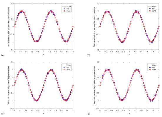
Figure 1. The exact solution and its approximate solution of Example 1 for $\epsilon =0.05$. (a) $\alpha =0.2$, (b) $\alpha =0.5$, (c) $\alpha =0.7$, (d) $\alpha =0.9$.

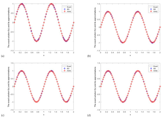
Figure 2. The exact solution and its approximate solution of Example 1 for $\epsilon =0.01$. (a) $\alpha =0.2$, (b) $\alpha =0.5$, (c) $\alpha =0.7$, (d) $\alpha =0.9$.

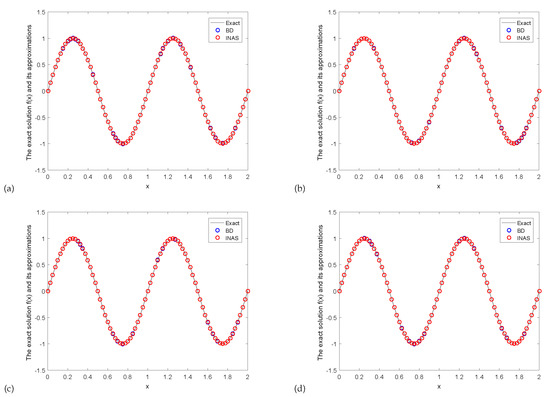
Figure 3. The exact solution and its approximate solution of Example 1 for $\epsilon =0.005$. (a) $\alpha =0.2$, (b) $\alpha =0.5$, (c) $\alpha =0.7$, (d) $\alpha =0.9$.

Table 1. Comparison between the relative root mean square errors of the exact solution and the regularization solution of Example 1 for various values of $\alpha$ and $\epsilon$.

			$\mathit{\alpha }=0.2$	$\mathit{\alpha }=0.5$	$\mathit{\alpha }=0.7$	$\mathit{\alpha }=0.9$
$\zeta \left(f\right)$	$\epsilon =0.05$	BD	0.0410	0.0312	0.0272	0.0288
		INAS	0.0141	0.0190	0.0193	0.0151
	$\epsilon =0.01$	BD	0.0099	0.0063	0.0065	0.0059
		INAS	0.0039	0.0059	0.0030	0.0019
	$\epsilon =0.005$	BD	0.0046	0.0032	0.0027	0.0027
		INAS	0.0023	0.0021	0.0016	0.0017

Table 2. Comparison of the number of iterations for the exact solution and the regularization solution of Example 1 for various values of $\alpha$ and $\epsilon$.

			$\mathit{\alpha }=0.2$	$\mathit{\alpha }=0.5$	$\mathit{\alpha }=0.7$	$\mathit{\alpha }=0.9$
Number of iterations (m)	$\epsilon =0.05$	BD	14362	362	56	31
		INAS	26,366	3623	1529	763
	$\epsilon =0.01$	BD	19,988	480	73	39
		INAS	35,055	4592	2159	1026
	$\epsilon =0.005$	BD	22,117	534	80	43
		INAS	37,551	5362	2374	1070

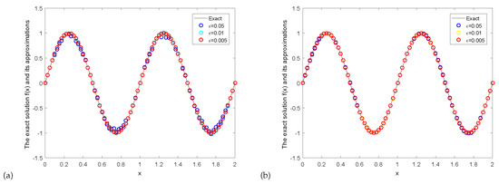
Figure 4. The exact solution and its approximate solution of Example 1 with $\alpha =0.6$ for $\epsilon =0.05,0.01,0.005$. (a) BD: m = 92, 135, 154, $\zeta \left(f\right)$ = 0.0714, 0.0020, 0.0007; (b) INAS: m = 2369, 3181, 3543, $\zeta \left(f\right)$ = 0.0029, 0.0004, 8.9000 × ${10}^{-5}$.

Figure 5, Figure 6 and Figure 7 show a comparison of the exact solution $f\left(x\right)$ and its approximate solution $f^{m,\delta }\left(x\right)$ between BD and INAS in the iterative form of Example 2 for the relative error levels $\epsilon =0.05,0.01,0.005$ with various values of $\alpha =0.2,0.5,0.7,0.9$. Table 3 shows a comparison of the relative root mean square errors $\zeta \left(f\right)$ for the exact solution and the regularization solution of Example 2 for various values of $\alpha =0.2,0.5,0.7,0.9$ and $\epsilon =0.05,0.01,0.005$. Table 4 shows a comparison of the number of iterations $\left(m\right)$ for the exact solution and the regularization solution of Example 2 for various values of $\alpha =0.2,0.5,0.7,0.9$ and $\epsilon =0.05,0.01,0.005$. Figure 8 shows a comparison between the exact solution and the regularization solution of the two iterative methods for $\epsilon =0.05,0.01,0.005$ under $\alpha =0.8$.

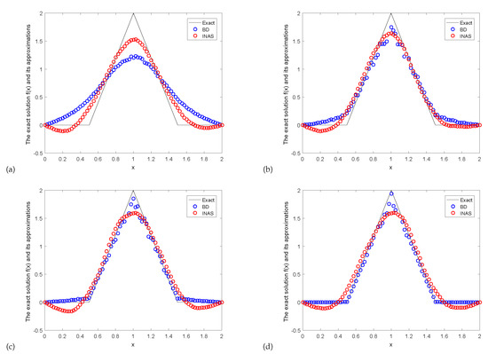
Figure 5. The exact solution and its approximate solution of Example 2 for $\epsilon =0.05$. (a) $\alpha =0.2$, (b) $\alpha =0.5$, (c) $\alpha =0.7$, (d) $\alpha =0.9$.

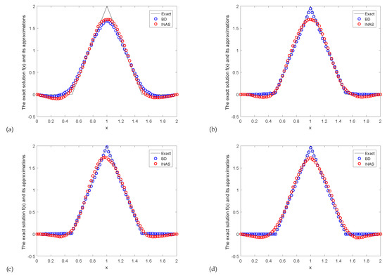
Figure 6. The exact solution and its approximate solution of Example 2 for $\epsilon =0.01$. (a) $\alpha =0.2$, (b) $\alpha =0.5$, (c) $\alpha =0.7$, (d) $\alpha =0.9$.

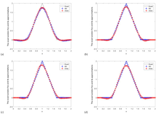
Figure 7. The exact solution and its approximate solution of Example 2 for $\epsilon =0.005$. (a) $\alpha =0.2$, (b) $\alpha =0.5$, (c) $\alpha =0.7$, (d) $\alpha =0.9$.

Table 3. Comparison of the relative root mean square errors for the exact solution and the regularization solution of Example 2 for various values of $\alpha$ and $\epsilon$.

			$\mathit{\alpha }=0.2$	$\mathit{\alpha }=0.5$	$\mathit{\alpha }=0.7$	$\mathit{\alpha }=0.9$
$\zeta \left(f\right)$	$\epsilon =0.05$	BD	0.3672	0.1441	0.0845	0.0734
		INAS	0.1910	0.1360	0.1579	0.1500
	$\epsilon =0.01$	BD	0.1106	0.0288	0.0159	0.0169
		INAS	0.0963	0.0849	0.0826	0.0905
	$\epsilon =0.005$	BD	0.0748	0.0170	0.0076	0.0077
		INAS	0.0641	0.0576	0.0638	0.0690

Table 4. Comparison of the number of iterations for the exact solution and the regularization solution of Example 2 for various values of $\alpha$ and $\epsilon$.

			$\mathit{\alpha }=0.2$	$\mathit{\alpha }=0.5$	$\mathit{\alpha }=0.7$	$\mathit{\alpha }=0.9$
Number of iterations (m)	$\epsilon =0.05$	BD	926	88	21	14
		INAS	3822	638	265	172
	$\epsilon =0.01$	BD	4470	198	36	23
		INAS	12,486	2738	1127	550
	$\epsilon =0.005$	BD	6502	241	43	27
		INAS	25,343	4368	1538	765

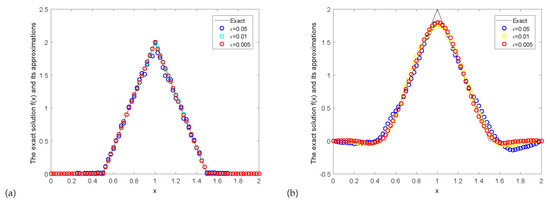
Figure 8. The exact solution and its approximate solution of Example 2 with $\alpha =0.8$ for $\epsilon =0.05,0.01,0.005$. (a) BD: m = 16, 26, 30, $\zeta \left(f\right)$ = 0.0694, 0.0027, 7.3236 ×${10}^{-4}$; (b) INAS: m = 337, 1043, 1565, $\zeta \left(f\right)$ = 0.5461, 0.2424, 1403.

Figure 9 and Figure 10 show a comparison of the exact solution $f\left(x\right)$ and its approximate solution $f^{m,\delta }\left(x\right)$ between BD and INAS in the iterative form of Example 3 for the relative error levels $\epsilon =0.05,0.01$ with various values of $\alpha =0.2,0.5,0.7,0.9$. Table 5 shows a comparison of the relative root mean square errors $\zeta \left(f\right)$ of the exact solution and the regularization solution of Example 3 for various values of $\alpha =0.2,0.5,0.7,0.9$ and $\epsilon =0.05,0.01$. Table 6 shows a comparison of the number of iterations $\left(m\right)$ for the exact solution and the regularization solution of Example 3 for various values of $\alpha =0.2,0.5,0.7,0.9$ and $\epsilon =0.05,0.01$. Figure 11 shows a comparison between the exact solution and the regularization solution of the two iterative methods for $\epsilon =0.05,0.01,0.005$ under $\alpha =0.95$.

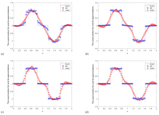
Figure 9. The exact solution and its approximate solution of Example 3 for $\epsilon =0.05$. (a) $\alpha =0.2$, (b) $\alpha =0.5$, (c) $\alpha =0.7$, (d) $\alpha =0.9$.

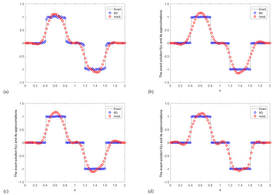
Figure 10. The exact solution and its approximate solution of Example 3 for $\epsilon =0.01$. (a) $\alpha =0.2$, (b) $\alpha =0.5$, (c) $\alpha =0.7$, (d) $\alpha =0.9$.

Table 5. Comparison of the relative root mean square errors for the exact solution and the regularization solution of Example 3 for various values of $\alpha$ and $\epsilon$.

			$\mathit{\alpha }=0.2$	$\mathit{\alpha }=0.5$	$\mathit{\alpha }=0.7$	$\mathit{\alpha }=0.9$
$\zeta \left(f\right)$	$\epsilon =0.05$	BD	0.1850	0.0535	0.0354	0.0388
		INAS	0.3693	0.3316	0.2884	0.3108
	$\epsilon =0.01$	BD	0.0426	0.0100	0.0071	0.0066
		INAS	0.2641	0.2838	0.2729	0.2441

Table 6. Comparison of the number of iterations for the exact solution and the regularization solution of Example 3 for various values of $\alpha$ and $\epsilon$.

			$\mathit{\alpha }=0.2$	$\mathit{\alpha }=0.5$	$\mathit{\alpha }=0.7$	$\mathit{\alpha }=0.9$
Number of iterations (m)	$\epsilon =0.05$	BD	14,090	256	41	23
		INAS	24,384	6491	6714	2243
	$\epsilon =0.01$	BD	47,555	420	56	32
		INAS	275,527	30,496	15,463	15,362

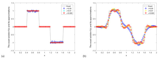
Figure 11. The exact solution and its approximate solution of Example 3 with $\alpha =0.95$ for $\epsilon =0.05,0.01,0.005$. (a) BD: m = 43,62,71, $\zeta \left(f\right)$ = 0.0443, 0.0031, 5.9184 ×${10}^{-4}$; (b) INAS: m = 1841, 20,875, 28,442, $\zeta \left(f\right)$ = 0.3082, 0.2395, 0.2069.

5. Conclusions

In this paper, an inverse problem to determine the initial value problem of the homogeneous Rayleigh–Stokes equation for a generalized second-grade fluid with the Riemann–Liouville fractional derivative model is studied. The Landweber iterative regularization method is used to solve the ill-posed problem. Under a conditional stability result, we obtain the convergent error estimates between the exact solution and the regularization solution by using an a priori regularization parameter choice rule and an a posteriori regularization parameter choice rule. Finally, three numerical examples are given to illustrate the effectiveness of this method. In the future, we will consider the other fractional derivative model of the homogeneous Rayleigh–Stokes equation for a generalized second-grade fluid and consider the inverse problem of identifying the unknown source and initial value for $1<\alpha <2$.

References

- Baleanu, D.; Jajarmi, A.; Mohammadi, H.; Rezapour, S. A new study on the mathematical modelling of human liver with Caputo-Fabrizio fractional derivative. Chaos Solitons Fract. 2020, 134, 109705. [Google Scholar] [CrossRef]
- Rezapour, S.; Mohammadi, H.; Jajarmi, A. A new mathematical model for Zika virus transmission. Adv. Differ. Eq. 2020, 2020, 589. [Google Scholar] [CrossRef]
- Baleanu, D.; Mohammadi, H.; Rezapour, S. Analysis of the model of HIV-1 infection of CD4+ T-cell with a new approach of fractional derivative. Adv. Differ. Eq. 2020, 2020, 71. [Google Scholar] [CrossRef] [Green Version]
- Tuan, N.H.; Ganji, R.M.; Jafari, H. A numerical study of fractional rheological models and fractional Newell-Whitehead-Segel equation with non-local and non-singular kernel. Chin. J. Phys. 2020, 68, 308–320. [Google Scholar] [CrossRef]
- Nikan, O.; Jafari, H.; Golbabai, A. Numerical analysis of the fractional evolution model for heat flow in materials with memory. Alex. Eng. J. 2020, 59, 2627–2637. [Google Scholar] [CrossRef]
- Ganji, R.M.; Jafari, H.; Baleanu, D. A new approach for solving multi variable orders differential equations with Mittag-Leffler kernel. Chaos Solitons Fract. 2020, 130, 109405. [Google Scholar] [CrossRef]
- Baleanu, D.; Etemad, S.; Rezapour, S. A hybrid Caputo fractional modeling for thermostat with hybrid boundary value conditions. Bound Value Probl. 2020, 2020, 64. [Google Scholar] [CrossRef] [Green Version]
- Shen, F.; Tan, W.; Zhao, Y.; Masuoka, T. The Rayleigh–Stokes problem for a heated generalized second grade fluid with fractional derivative model. Nonlinear Anal. Real World Appl. 2006, 7, 1072–1080. [Google Scholar] [CrossRef]
- Fetecau, C.; Jamil, M.; Fetecau, C.; Vieru, D. The Rayleigh–Stokes problem for an edge in a generalized Oldroyd-B fluid. Z. Angew. Math. Phys. 2009, 60, 921–933. [Google Scholar] [CrossRef]
- Song, D.Y.; Jiang, T.Q. Study on the constitutive equation with fractional derivative for the viscoelastic fluids-Modified Jeffreys model and its application. Rheol. Acta 1998, 37, 512–517. [Google Scholar] [CrossRef]
- Zhao, C.L.; Yang, C. Exact solutions for electro-osmotic flow of viscoelastic fluids in rectangular micro-channels. Appl. Math. Comput. 2009, 211, 502–509. [Google Scholar] [CrossRef]
- Khan, M. The Rayleigh–Stokes problem for an edge in a viscoelastic fluid with a fractional derivative model. Nonlinear Anal. Real World Appl. 2009, 10, 3190–3195. [Google Scholar] [CrossRef]
- Khan, M.; Anjum, A.; Qi, H.; Fetecau, C. On exact solutions for some oscillating motions of a generalized Oldroyd-B fluid. Z. Angew. Math. Phys. 2010, 61, 133–145. [Google Scholar] [CrossRef]
- Chen, C.M.; Liu, F.; Anh, V. Numerical analysis of the Rayleigh–Stokes problem for a heated generalized second grade fluid with fractional derivatives. Appl. Math. Comput. 2008, 204, 340–351. [Google Scholar] [CrossRef] [Green Version]
- Chen, C.M.; Liu, F.; Burrage, K.; Chen, Y. Numerical methods of the variable-order Rayleigh–Stokes problem for a heated generalized second grade fluid with fractional derivative. IMA J. Appl. Math. 2013, 78, 924–944. [Google Scholar] [CrossRef]
- Elyas, S.; Ahmad, J. Rayleigh–Stokes problem for a heated generalized second grade fluid with fractional derivatives: A stable scheme based on spectral meshless radial point interpolation. Eng. Comput. 2017, 34, 77–90. [Google Scholar]
- Dehghan, M.; Abbaszadeh, M. A finite element method for the numerical solution of Rayleigh–Stokes problem for a heated generalized second grade fluid with fractional derivatives. Eng. Comput. 2017, 33, 1–19. [Google Scholar] [CrossRef]
- Nikan, O.; Golbabai, A.; Tenreiro Machado, J.A.; Nikazad, T. Numerical solution of the fractional Rayleigh–Stokes model arising in a heated generalized second-grade fluid. Eng. Comput. 2021. [Google Scholar] [CrossRef]
- Chen, C.M.; Liu, F.; Turner, I.; Anh, V. Numerical methods with fourth-order spatial accuracy for variable-order nonlinear Stokes’ first problem for a heated generalized second grade fluid. Comput. Math. Appl. 2011, 62, 971–986. [Google Scholar] [CrossRef] [Green Version]
- Hoang, L.N.; Huy, T.N.; Kirane, M.; Xuan, T.D.D. Identifying initial condition of the Rayleigh–Stokes problem with random noise. Math. Methods Appl. Sci. 2019, 42, 1561–1571. [Google Scholar]
- Yang, F.; Zhang, P.; Li, X.X. The truncation method for the Cauchy problem of the inhomogeneous Helmholtz equation. Appl. Anal. 2019, 98, 991–1004. [Google Scholar] [CrossRef]
- Yang, F.; Fan, P.; Li, X.X. Fourier truncation regularization method for a three-dimensional Cauchy problem of the modified Helmholtz equation with perturbed wave number. Mathematics 2019, 7, 705. [Google Scholar] [CrossRef] [Green Version]
- Wang, J.G.; Wei, T.; Zhou, Y.B. Tikhonov regularization method for a backward problem for the time-fractional diffusion equation. Appl. Math. Model. 2013, 37, 8518–8532. [Google Scholar] [CrossRef]
- Feng, X.L.; Eldén, L. Solving a Cauchy problem for a 3D elliptic PDE with variable coefficients by a quasi-boundary-value method. Inverse Probl. 2014, 30, 015005. [Google Scholar] [CrossRef]
- Yang, F.; Wang, N.; Li, X.X. A quasi-boundary regularization method for identifying the initial value of time-fractional diffusion equation on spherically symmetric domain. J. Inverse Ill-Posed Probl. 2019, 27, 609–621. [Google Scholar] [CrossRef]
- Yang, F.; Sun, Y.R.; Li, X.X. The quasi-boundary value method for identifying the initial value of heat equation on a columnar symmetric domain. Numer. Algorithms 2019, 82, 623–639. [Google Scholar] [CrossRef]
- Zhang, H.W.; Qin, H.H.; Wei, T. A quasi-reversibility regularization method for the Cauchy problem of the Helmholtz equation. Int. J. Comput. Math. 2011, 88, 839–850. [Google Scholar] [CrossRef]
- Yang, F.; Fu, C.L. The quasi-reversibility regularization method for identifying the unknown source for time fractional diffusion equation. Appl. Math. Model. 2015, 39, 1500–1512. [Google Scholar] [CrossRef]
- Yang, F.; Fu, C.L.; Li, X.X. A mollification regularization method for unknown source in time-fractional diffusion equation. Int. J. Comput. Math. 2014, 91, 1516–1534. [Google Scholar] [CrossRef]
- Xiong, X.T.; Fu, C.L.; Li, H.F. Fourier regularization method of a sideways heat equation for determining surface heat flux. J. Math. Anal. Appl. 2006, 317, 331–348. [Google Scholar] [CrossRef] [Green Version]
- Li, X.X.; Lei, J.L.; Yang, F. An a posteriori Fourier regularization method for identifying the unknown source of the space-fractional diffusion equation. J. Inequal. Appl. 2014, 2014, 1–13. [Google Scholar] [CrossRef] [Green Version]
- Yang, F.; Fu, C.L.; Li, X.X. The Fourier regularization method for identifying the unknown source for the modified Helmholtz equation. Acta Math. Sin. 2014, 34, 1040–1047. [Google Scholar]
- Yang, F.; Zhang, Y.; Li, X.X. Landweber iterative method for identifying the initial value problem of the time-space fractional diffusion-wave equation. Numer. Algorithms 2019, 83, 1509–1530. [Google Scholar] [CrossRef]
- Yang, F.; Ren, Y.P.; Li, X.X. Landweber iteration regularization method for identifying unknown source on a columnar symmetric domain. Inverse Probl. Sci. Eng. 2018, 26, 1109–1129. [Google Scholar] [CrossRef]
- Yang, F.; Liu, X.; Li, X.X. Landweber iterative regularization method for identifying the unknown source of the modified Helmholtz equation. Bound. Value Probl. 2017, 2017, 1–16. [Google Scholar] [CrossRef]
- Bazhlekova, E.; Jin, B.T.; Lazarov, R.; Zhou, Z. An analysis of the Rayleigh–Stokes problem for a generalized second-grade fluid. Numer. Math. 2015, 131, 1–31. [Google Scholar] [CrossRef] [PubMed] [Green Version]
- Engl, H.W.; Hanke, M.; Neubauer, A. Regularization of Inverse Problems; Kluwer Academic Publishers: Boston, MA, USA, 2019. [Google Scholar]
- Wu, C. Numerical solution for Stokes’ first problem for a heated generalized second grade fluid with fractional derivative. Appl. Numer. Math. 2009, 59, 2571–2583. [Google Scholar] [CrossRef]
- Yuste, S.B. Weighted average finite difference methods for fractional diffusion equations. J. Comput. Phys. 2006, 216, 264–274. [Google Scholar] [CrossRef] [Green Version]
Publisher’s Note: MDPI stays neutral with regard to jurisdictional claims in published maps and institutional affiliations. |
© 2021 by the authors. Licensee MDPI, Basel, Switzerland. This article is an open access article distributed under the terms and conditions of the Creative Commons Attribution (CC BY) license (https://creativecommons.org/licenses/by/4.0/).