Article

A Special Study of the Mixed Weighted Fractional Brownian Motion

1
Ministry of Education, General Directorate of Education in Saladin, Tikrit 34001, Iraq
2
Department of Mathematics, COMSATS University Islamabad, Abbottabad 22060, Pakistan
3
Nonlinear Analysis and Applied Mathematics (NAAM)-Research Group, Department of Mathematics, Faculty of Science, King Abdulaziz University, P.O. Box 80203, Jeddah 21589, Saudi Arabia
4
Department of Mathematical Statistics, Faculty of Graduate Studies for Statistical Research, Cairo University, Giza 12613, Egypt
5
Mathematics Department, Faculty of Exact Sciences and Informatics, Hassiba Benbouali University, Chlef 02180, Algeria
*
Author to whom correspondence should be addressed.
Fractal Fract. 2021, 5(4), 192; https://doi.org/10.3390/fractalfract5040192
Submission received: 18 September 2021 / Revised: 16 October 2021 / Accepted: 20 October 2021 / Published: 31 October 2021

Abstract

:
In this work, we present the analysis of a mixed weighted fractional Brownian motion, defined by η t : = B t + ξ t , where B is a Brownian motion and ξ is an independent weighted fractional Brownian motion. We also consider the parameter estimation problem for the drift parameter θ > 0 in the mixed weighted fractional Ornstein–Uhlenbeck model of the form X 0 = 0 ; X t = θ X t d t + d η t . Moreover, a simulation is given of sample paths of the mixed weighted fractional Ornstein–Uhlenbeck process.

1. Introduction

Over the course of the last two decades, the investigation of a system of particles moving in R d under the influence of a symmetric α -stable Lèvy noise, 0 < α 2 , has attracted many scholars’ attention (e.g., [1,2,3,4,5]). Research on certain particle systems and their occupational time-fluctuation limits has revealed new types of centered Gaussian processes that are self-similar and have long-range dependences [6]. The particle systems determine the values of the parameters in these stochastic processes. One of the most important of these stochastic processes is the weighted fractional Brownian motion (wfBm). Bojdecki et al. [6] were the first to bring it up in 2007, and called it “a weighted fractional Brownian motion” because of the weight function u a that appears in its covariance function
k ( s , t ) = 0 s t u a [ ( t u ) b + ( s u ) b ] d u , t 0 ,
where a , b satisfy
1 < a , 1 > | b | , 1 + a > | b | .
For a = 0 , 1 < b < 1 , wfBm corresponds to the celebrated fractional Brownian motion (fBm) with Hurst index b + 1 2 , as well as to the well-known Brownian motion (Bm) when a = 0 , b = 0 . Many studies have been devoted to the weighted fractional Brownian motion and the related Ornstein–Uhlenbeck process, for instance [7,8,9].
Parameter estimation for dynamical models is the most essential component of the subject for engineers and applied scientists [10]. In recent years, the problem of statistical estimation for Gaussian Ornstein–Uhlenbeck processes has piqued the interest of various scholars. In the ergodic case where θ < 0 , several works, such as [11,12] and the references therein, have focused on the statistical estimation of the parameter θ . Furthermore, in the non-ergodic scenario corresponding to θ > 0 , the estimation of parameter θ has been explored using the least squares method, as can be seen in [8,13,14,15,16,17] and its references.
Recently, the mixed Gaussian noise has become of interest because of its applications in many different fields, such as engineering [18], mathematical finance [19,20] and so on. These mixtures can solve problems in mathematical finance and option pricing. Cheridito [19] has pointed out that the mixed fractional Brownian motion (mfBm) is equivalent to Bm for 3 4 < H 1 , which was applied by Cheridito to obtain a new type of Samuelson model, which is arbitrage-free and complete. Moreover, in [20], the pricing of Bermuda options on zero-coupons bound for the mixed fractional Vasicek process has been considered, for H ( 3 4 , 1 ) . The authors applied the Akaike information criterion (AIC) on US interest rates from January 2015 to May 2019 to show that the Vasicek model driven by mfBm is more appropriate than the standard model with fBm.
Our motivation behind introducing the mixed-weighted fractional Brownian motion (mwfBm) comes from the fact that the filtration of wfBm does not satisfy the usual assumptions, which means that this cannot be a semimartingale; however this mixture, together with the asymptotic stationary properties for wfBm, opens up the possibility of mwfBm being martingale or equivalent to Bm, as it is the same as mfBm (see Remark 1).
Inspired by the aforementioned monographs and facts, in this work, we begin by introducing a new stochastic process named as the mixed weighted fractional Brownian motion and establish the stochastic integral and the canonical representation for such process. In addition, we apply this process to one of the most interesting problem in mathematical statistics which is parameter estimation problem, such that we investigate the problem of parameter estimation for Ornstein–Uhlenbek process in which the dynamics follows mwfBm. Consequently, new results have been established for the proposed estimator of parameter θ that are different from those that have previously been obtained for both fBm and wfBm (see Section 3). On the other hand, we used the most recent results for the numerical simulation (such as in [21,22,23,24]) to discuss the simulation of the sample paths of the mixed weighted fractional Ornstein–Uhlenbeck process.
The remainder of this paper is organised in the following manner. In the second section, some notions and basic facts related to the mwfBm and its stochastic calculus are presented. Section 3 focuses on the problem of estimating the drift parameter for the non-ergodic mixed weighted fractional Ornstein–Uhlenbeck process (mwfOUP). We provide a numerical simulation for the solution of the weighted fractional Ornstein–Uhlenbeck model in Section 5. The results of numerical simulations are summarised and discussed in Section 6. Finally, the last section highlights the results of this paper.

2. Notions and Auxiliary Results

This section introduces some fundamental concepts and facts about the mixed weighted fractional Brownian motion and its stochastic calculus.
First, we provide a definition for mwfBm.
Definition 1.
The stochastic process η = ( η t ) t 0 will be called a mixed-weighted fractional Brownian motion (mwfBm) if it is described by the linear combination of a weighted fractional Brownian motion and an independent standard Brownian motion, namely
η t : = B t + ξ t ,
where B is Bm and ξ is the independent wfBm and the parameters a , b of the wfBm satisfy condition (2).
In the following, we consider ( Ω , F , { F t } t 0 , P ) to be a complete-probability space equipped with a natural filtration { F t } t 0 , where F t stands for the σ -algebra generated by η and F 0 indicates the set of all P-null sets.

A Canonical Innovation Representation for mwfBm

Let M = ( M t ) 0 t T be a fundamental martingale and M t be its quadratic variance, such that, for t 0 ,
M t = 0 t g ( s , t ) d η s , M t = 0 t g ( s , t ) d s = 0 t g 2 ( s , s ) d s ,
where g ( s , t ) can solve the following equation:
g ( s , t ) = 1 0 t g ( u , t ) K ( u , s ) d u ,
where K ( u , s ) : = b ( t s ) a ( t s t s ) b 1 ; t [ 0 , T ] . Then, by using the same strategy of Theorem 2.4 in [25], we have
η t : = 0 t G ( s , t ) d M s ; t [ 0 , T ] ,
with
G ( s , t ) : = 1 1 g ( s , s ) 0 t R ( t 0 , s ) d t 0 ; s t [ 0 , T ] R ( s , t ) : = g ( s , t ) t × 1 g ( t , t ) ; s t .
We introduce the function φ : [ 0 , T ] × [ 0 , T ] [ 0 , T ] , which is defined as
φ ( t , s ) = 2 k ( t , s ) t s = ( t s ) a ( t s t s ) b 1 , t [ 0 , T ] .
Let f : [ 0 , T ] [ 0 , T ] be “a Borel measurable function” and define the space
L φ 2 ( [ 0 , T ] ) = { f : f L φ 2 ( [ 0 , T ] ) 2 = 0 T 0 T f ( t ) f ( s ) φ ( t , s ) d s d t + 0 T f 2 ( t ) d t < } ,
which, under the following inner product formula, becomes a “separable Hilbert space”
f , g L φ 2 ( [ 0 , T ] ) = 0 T 0 T f ( t ) g ( s ) φ ( t , s ) d s d t + 0 T f ( t ) g ( t ) d t , f , g L φ 2 ( [ 0 , T ] ) : = H .
Let ψ H ; then, from [26,27] and following the same technique as used in Section 2 of [25] and Section 2.2 of [28], we obtain
0 T ψ ( t ) d η t = 0 T [ t 0 T ψ ( t ) G t ( t 0 , t ) d t + ψ ( t 0 ) G ( t 0 , t 0 ) ] d M t 0 ,
where M and G are given by Equations (4) and (6), respectively.
Moreover, there exists a Brownian motion B = { B t } t 0 with the same filtration of η ; hence,
0 T ψ ( t ) d η t = 0 T [ t 0 T g ( t 0 , t 0 ) G t ( t 0 , t ) ψ ( t ) d t + ψ ( t 0 ) ] d B t 0 ,
where g is as defined below in (5).
Consider the operator G * : H L 2 [ 0 , T ] given by
( G * ψ ) ( t 0 ) = t 0 T g ( t 0 , t 0 ) G t ( t 0 , t ) ψ ( t ) d t + ψ ( t 0 ) .
We will now define “the divergence integral” with respect to mwfBm.
Definition 2.
Let u = u ( ω ) : [ 0 , T ] H be a random variable and G * u be Skorohod–integral in terms of Bm B. Then, the Wiener integral of u in terms of η is given via
η ( u ) : = 0 T ( G * u ) ( t 0 ) δ B t 0 = 0 T u ( t ) d η t .
in the following, we look at the set E of smooth random variables, which is described as
F ( ω ) = g 0 T ψ 1 ( t ) d η ( t ) , , 0 T ψ n ( t ) d η ( t ) ,
where g C b ( [ 0 , T ] ) and ψ i H , i 1 . The following definition provides a representation of a Malliavin derivative related to the process η .
Definition 3.
The Malliavin derivative D t η F of a smooth random variable F is a H -valued random variable, such that
D t η F = i = 1 n g x i 0 T ψ 1 ( t ) d η ( t ) , . . . , 0 T ψ n ( t ) d η ( t ) ψ i ( t ) , t 0 .
the operator D t η is a closable operator in L p ( Ω ) , so that D t η : L p ( Ω ) L p ( Ω , H ) . In addition, the iteration of the Malliavin derivative D η is indicated by D t η , k , 1 k . For 1 p , the Sobolev space D k , p indicates the closure of the set E in terms of the following norm
F k , p p = E | F | p + E i = 1 k D t η , i F H i p ,
where “⨂” denotes the tensor product.
Definition 4.
Let δ η be the adjoint operator of D η . We call δ η the Skorohod integral operator w.r.t η, δ η is an unbounded operator on the space L 2 ( Ω ; H ) , and the domain of δ η , which is indicated by D o m ( δ η ) , represents a class of H -valued square integrable random variables. If u D o m ( δ η ) , then the Skorohod integral w.r.t η is denoted by
δ η ( u ) : = 0 T u ( t ) δ η t .
Definition 5.
Consider v to be a stochastic process with integrable trajectories and the below limits exist in terms of probability. Then
  • The symmetric integral of v w.r.t η, is given by
    0 T v ( t ) d η t : = lim ϵ 0 1 2 ϵ 0 T v ( t ) [ η ( t + ϵ ) η ( t ϵ ) ] d t .
  • The forward integral of v in terms of η, is defined by
    0 T v ( t ) d η t : = lim ϵ 0 1 ϵ 0 T v ( t ) η ( t + ϵ ) η ( t ) ϵ d t ,
  • The backward integral of v in terms of η, can be expressed as
    0 T v ( t ) d + η t : = lim ϵ 0 1 ϵ 0 T v ( t ) η ( t ϵ ) η ( t ) ϵ d t ,
Lemma 1.
Assume that the process ( v t ) 0 t T is living in the space D 1 , 2 , and the following assertions hold true:
  • 0 T 0 T | D s η v ( t ) | φ ( t , s ) d s d t < , a.s,
  • 0 T | D t η v ( t ) | d t < , a.s, D s η v ( t ) = 0 if t < s ,
here D t η v ( t ) means D s η v ( t ) when s = t . Then
0 T v ( t ) d η t : = δ η ( v ) + 0 T 0 T D s η v ( t ) φ ( s , t ) d s d t + 1 2 0 T D t η v ( t ) d t .
Proof. 
We use the same arguments that are used to prove Lemma 2.7 in [28]. □
Remark 1.
Recently, Cai et al. [28] pointed out that the mixed fractional Brownian motion has an explicit form of its fundamental martingale in the case of H < 1 2 . This was also preceded by the monograph [19], which revealed using Theorem 1 of [29] that, for H ( 3 4 , 1 ] , the mfBm is the same as Bm. These facts open a new problem regarding the possibility of the mixed Gaussian noises being martingales or equivalent to Bm. For wfBm, as its filtration does not satisfy the usual assumptions, ξ cannot be a semimartingale (see Theorem 2.4 of [6]). Meanwhile, wfBm has the property of asymptotic stationary increments for long time intervals, that is to say
lim T T ( 1 + a + b ) E ( ξ t + T ξ t ) 2 = 2 0 1 u a ( 1 u ) b d u ,
and we know that (see Theorem 1.7 in [19]) mfBm has been shown to be equivalent to Bm based on the property of stationary increments. This opens up the possibility of mwfBm being equivalent to Bm. For the sake of brevity, we will not pursue further details here, but leave this problem open for future research.

3. Least Square Estimator for the mwfOU Process

This section deals with the problem of estimating drift parameter for the non-ergodic mwfOU process based on continuous observation { X t , 0 t T } . The dynamic of this process is
X 0 = 0 ; d X t = θ X t d t + d η t , t 0 ,
where 0 < θ is considered to be an unknown parameter. Moreover, the explicit solution for (7) can be written as
X t = e θ t 0 t e θ s d η s , t 0 .
Consider the least square type estimator for (7), which is defined as follows:
θ ^ T = 0 T X t d X t 0 T X t 2 d t , t 0 ,
from (7) and (8) and using Lemma 2.6, we obtain
0 T X t δ η t = 0 T X t d η t b 0 T 0 t exp ( θ ( t s ) ) ( t s ) a ( t s t s ) b 1 d s d t T 2 ,
Thus, we obtain the following expression for the LSE
θ ^ T = X t 2 2 0 T X t 2 d t b 0 T 0 t exp ( θ ( t s ) ) ( t s ) a ( t s t s ) b 1 d s d t 0 T X t 2 d t T 0 T X t 2 d t .
It is clear that the quadratic variation in the mwfOU process is not zero, which is the essential push for us to consider the mixed case.
Now, it is obvious, as T ,
e 2 θ T b 0 T 0 t exp ( θ ( t s ) ) ( t s ) a ( t s t s ) b 1 d s d t 0 T X t 2 d t 0 ,
and
e 2 θ T T 0 T X t 2 d t 0 ,
hence, it follows that (10) can be written as
θ ˇ T = X t 2 2 0 T X t 2 d t .

The Behavior of LSE θ ˇ T

The last square estimator’s strong consistency and asymptotic distribution for a class of Gaussian Ornstein–Uhlenbeck processes has recently been established by [13]. In our case, due the fact that the combination of two Gaussian processes is also Gaussian, the methodology used by [13] can be applied for the mwfOU process.
According to Theorem 3.1 in [7] and the properties of Bm, we have
E [ η t 2 ] E [ ( B t + ξ t ) 2 ] = E [ B t 2 ] + E [ ξ t 2 ] = t + 2 β ( 1 + a , 1 + b ) t ( a + b + 1 ) c γ + t .
where c is a positive constant, γ : = a + b + 1 and β ( m , n ) = 0 1 x m 1 ( 1 x ) n 1 d x represents the usual Beta function.
In addition, we have
E [ η t η s ] 2 E [ η t 2 ] + E [ η s 2 ] = E [ B t 2 ] + E [ ξ t 2 ] + E [ B s 2 ] + E [ ξ s 2 ] = t + 2 β ( 1 + a , 1 + b ) t ( a + b + 1 ) + s + 2 β ( 1 + a , 1 + b ) s ( a + b + 1 ) = t + s + 2 β ( 1 + a , 1 + b ) ( t ( a + b + 1 ) + s ( a + b + 1 ) ) c t γ + | t s | .
Here the the last inequity stems from the fact that ( t + s ) | t s | , 0 < s t , and γ : = a + b + 1 .
Next, we let X t to be
X t = X t ( 1 ) + X t ( 2 ) ; d X t ( 1 ) : = θ X t ( 1 ) d t + d B t ; 0 t T , d X t ( 2 ) : = θ X t ( 2 ) d t + d ξ t ; 0 t T ,
Define the process Z t : = 0 t e θ s η s d s ; t 0 . Then, using the decomposition of X in (12) together with Lemma 2.1 of [13] and Theorem 3.1 of [7], we obtain
X T 2 θ 2 Z 2 ,
and
e 2 θ T 0 t X t 2 d t θ 2 Z 2 ,
as T . From this discussion, and by virtue of Lemma 2.1 of [13] and Theorem 3.1 of [7], we deduce that the estimator θ ˇ T is almost consistent with the parameter θ , as T and it is asymptotically Cauchy, as T . This is the message conveyed by the next theorem.
Theorem 1.
Let θ ˇ T be the estimator given by (11), if a , b satisfies the condition (2). Then, T
θ ˇ T θ . Moreover, e θ T ( θ ˇ T θ ) l a w 2 θ C ( 1 ) , as T , here C ( 1 ) is a standard Cauchy distribution with a probability density function given by 1 π ( 1 + x 2 ) with x R .

4. Numerical Simulations

This section focuses on the simulation of the sample paths of the mixed-weighted fractional Brownian motion and related Ornstein–Uhlenbeck process. To date, different algorithms have been used to simulate correlated Gaussian random variables (see, for instance, [21,22,30]). However, few works have studied the simulation of wfBm (see, for example, [8]). In our algorithm, we rely on the initial push outlined in Remark 2.3 of [6], in which the authors claimed that, in the case of b = 1 , the process ξ can be represented through Bm B, as follows:
ξ t = 0 t B r a d r
where a 0 . Moreover, we provide an algorithm for the simulation solution of the mwfOU process. Our simulation procedures are given below:
1.
Set the sample size N N and the time span T.
2.
Consider the uniform mesh with step-size h = T N and let 0 = t 0 < t 1 < < t N = T .
3.
Choose two values for each of the parameters θ , a .
4.
Compute the sample paths of ξ by
ξ ( t i + 1 ) = ξ ( t i ) + h i = 0 N 1 B ( t i ) a .
5.
Approximate the mwfOU process through
X ( t i + 1 ) = X ( t i ) + θ X ( t i ) h + ξ ( t i ) + B ( t i ) ; i = 0 , , N .
where ξ ( t i ) = ξ ( t i + 1 ) ξ ( t i ) and
B ( t i ) : = B ( t i + 1 ) B ( t i ) = t i + 1 t i × N ( 0 , 1 ) .
In the following, for different values of θ , a , we generate the sample paths of the mwfOU process.

5. Discussion

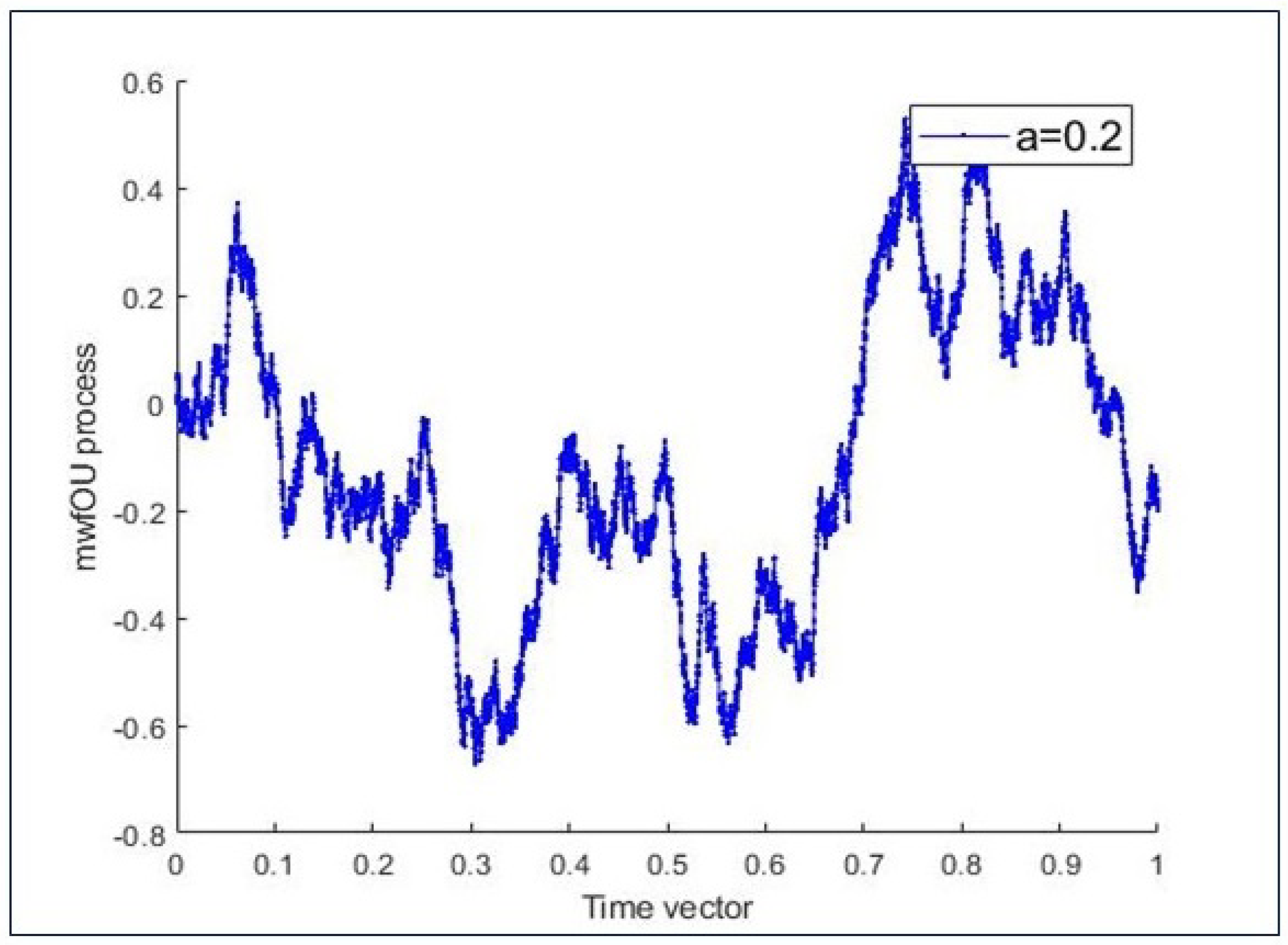
In this section, we discuss the previous numerical results. For different values of θ , a , we generate the sample paths of the mwfOU process that is shown in Figure 1 and Figure 2. From these simulations, we can observe that the characterisation of the sample paths of mwfOU process can be determined by the values of θ , a . In other words, we get smooth sample paths of X in the case of large values of θ , a . However, small values of θ and a make the sample paths of mwfOU process fluctuate more wildly. In Figure 1, we generate the sample paths of mwfOU process with θ = 2.5 , a = 2.5 , while we take θ = 0.5 , a = 0.2 in Figure 2.

6. Conclusions

We first introduced the mixed weighted fractional Brownian motion; then, the stochastic integral and canonical representation were established for the mixed weighted fractional Brownian motion. Moreover, we considered the parameter estimation problem for the drift parameter of the mixed weighted fractional Ornstein–Uhlenbeck model, and proved that the proposed estimator θ ˇ T is almost certainly consistent with the parameter θ , as T and is asymptotically Cauchy when T tends towards infinity. Finally, the simulation of the sample paths of the mixed-weighted fractional Ornstein–Uhlenbeck process is provided for different cases.

Author Contributions

Conceptualization, A.D.K.; methodology, A.D.K.; software, A.D.K.; validation, A.Z., S.D.; formal analysis, A.D.K.; investigation, A.D.K. writing—original draft preparation, A.D.K. and A.Z. and S.D.; writing—review and editing, A.D.K. and A.Z. and S.D.; supervision, T.S. and H.M.A.; project administration, M.A.; funding acquisition, T.S. All authors have read and agreed to the published version of the manuscript.

Funding

This research received no external funding.

Institutional Review Board Statement

Not applicable.

Informed Consent Statement

Not applicable.

Data Availability Statement

The authors confirm that the data supporting the findings of this study are available within the cited article.

Acknowledgments

The authors are very thankful to the anonymous reviewers.

Conflicts of Interest

The authors declare that there is no conflict of interest regarding the publication of this paper.

References

  1. Bojdecki, T.; Gorostiza, L.G.; Talarczyk, A. A long range dependence stable process and an infinite variance branching system. Ann. Probab. 2007, 35, 500–527. [Google Scholar] [CrossRef] [Green Version]
  2. Bojdecki, T.; Gorostiza, L.G.; Talarczyk, A. Limit theorems for occupation time fluctuations of branching systems I: Long-range dependence. Stoch. Process. Appl. 2006, 116, 1–18. [Google Scholar] [CrossRef] [Green Version]
  3. Bojdecki, T.; Gorostiza, L.G.; Talarczyk, A. Occupation time limits of inhomogeneous Poisson systems of independent particles. Stoch. Process. Their Appl. 2008, 118, 28–52. [Google Scholar] [CrossRef] [Green Version]
  4. Dawson, D.A.; Gorostiza, L.G.; Wakolbinger, A. Occupation time fluctuations in branching systems. J. Theoret. Probab. 2001, 14, 729–796. [Google Scholar] [CrossRef]
  5. Atangana, A. Mathematical model of survival of fractional calculus, critics and their impact: How singular is our world? Adv. Differ. Equ. 2021, 2021, 403. [Google Scholar] [CrossRef]
  6. Bojdecki, T.; Gorostiza, L.G.; Talarczyk, A. Some extensions of fractional Brownian motion and sub–fractional Brownian motion related to particle system. Electron. Commun. Probab. 2007, 12, 161–172. [Google Scholar] [CrossRef] [Green Version]
  7. Alsenafi, A.; Al-Foraih, M.; Es-Sebaiy, K. Least squares estimation for non-ergodic weighted fractional Ornstein–Uhlenbeck process of general parameters. arXiv 2020, arXiv:2002.06861. [Google Scholar]
  8. Cheng, P.; Shen, G.; Chen, Q. Parameter estimation for non–ergodic Ornstein–Uhlenbeck process driven by the weighted fractional Brownian motion. Adv. Differ. Equ. 2017, 366. [Google Scholar]
  9. Shen, G.; Yin, X.; Yan, L. Least squares estimation for Ornstein-Uhlenbeck processes driven by the weighted fractional Brownian motion. Acta Math Sci. 2016, 36, 394–408. [Google Scholar] [CrossRef]
  10. Van den Bos, A. Parameter Estimation for Scientists and Engineers; John Wiley & Sons: Hoboken, NJ, USA, 2007. [Google Scholar]
  11. Es-Sebaiy, K.; Viens, F. Optimal rates for parameter estimation of stationary Gaussian processes. Stoch. Process. Their Appl. 2019, 129, 3018–3054. [Google Scholar] [CrossRef] [Green Version]
  12. Hu, Y.; Nualart, D.; Zhou, H. Parameter estimation for fractional Ornstein–Uhlenbeck processes of general Hurst parameter. Stat. Inference Stoch. Process. 2019, 22, 111–142. [Google Scholar] [CrossRef] [Green Version]
  13. El-Machkouri, M.; Es-Sebaiy, K.; Ouknine, Y. Least squares estimator for non–ergodic Ornstein Uhlenbeck processes driven by Gaussian processes. J. Korean Stat. Soc. 2016, 45, 329341. [Google Scholar] [CrossRef] [Green Version]
  14. Khalaf, A.D.; Zeb, A.; Sabawi, Y.A.; Djilali, S.; Wang, X.J. Optimal rates for the parameter prediction of a Gaussian Vasicek process. Eur. Phys. J. Plus 2021, 136, 1–7. [Google Scholar]
  15. Guin, L.N.; Pal, S.; Chakravarty, S.; Djilali, S. Pattern dynamics of a reaction-diffusion predator-prey system with both refuge and harvesting. Int. J. Biomath. 2021, 14, 2050084. [Google Scholar] [CrossRef]
  16. Djilali, S.; Benahmadi, L.; Tridane, A.; Niri, K. Modeling the impact of unreported cases of the COVID-19 in the North African countries. Biology 2020, 9, 373. [Google Scholar] [CrossRef]
  17. Bentout, S.; Chen, Y.; Djilali, S. Global dynamics of an SEIR model with two age structures and a nonlinear incidence. Acta Appl. Math. 2021, 171, 1–27. [Google Scholar] [CrossRef]
  18. Kailath, T.; Poor, H.V. Detection of stochastic processes. IEEE Trans. Inform. Theory 1998, 44, 2230–2259. [Google Scholar] [CrossRef] [Green Version]
  19. Cheridito, P. Mixed fractional Brownian motion. Bernoulli 2001, 7, 913–934. [Google Scholar] [CrossRef]
  20. Mehrdoust, F.; Najafi, A.R.; Samimi, H. A mixed fractional Vasicek model and pricing Bermuda option on zero-coupon bonds. Sādhanā 2020, 2020, 45–58. [Google Scholar] [CrossRef]
  21. Khalaf, A.D.; Abouagwa, M.; Mustafa, A.; Wang, X. Stochastic Volterra integral equations with jumps and the strong superconvergence of the Euler–Maruyama approximation. J. Comput. Appl. Math. 2021, 15, 113071. [Google Scholar] [CrossRef]
  22. Sabawi, Y.A.; Pirdawood, M.A.; Khalaf, A.D. Semi-Implicit and Explicit Runge Kutta Methods for Stiff Ordinary Differential Equations. J. Phys. Conf. Ser. 2021, 1999, 012100. [Google Scholar] [CrossRef]
  23. Moghaddam, B.P.; Lopes, A.M.; Machado, J.A.T.; Mostaghim, Z.S. Computational scheme for solving nonlinear fractional stochastic differential equations with delay. Stoch. Anal. Appl. 2019, 37, 893–908. [Google Scholar] [CrossRef]
  24. Tesfay, A.; Tesfay, D.; Khalaf, A.D.; Brannan, J. Mean exit time and escape probability for the stochastic logistic growth model with multiplicative α-stable Lévy noise. Stochastics Dyn. 2021, 21, 2150016. [Google Scholar] [CrossRef]
  25. Cai, C.; Chigansky, P.; Kleptsyna, M. Mixed Gaussian process: A filtering approach. Ann Probab. 2016, 44, 3032–3075. [Google Scholar] [CrossRef]
  26. Khalaf, A.D.; Abouagwa, M.; Wang, X.J. Periodic averaging method for impulsive stochastic dynamical systems driven by fractional Brownian motion under non–Lipschitz condition. Adv. Differ. Equ. 2019, 526, 1–15. [Google Scholar] [CrossRef] [Green Version]
  27. Nualart, D. Malliavin Calculus and Related Topics; Springer: Berlin, Germany, 2006. [Google Scholar]
  28. Cai, C.; Wang, Q.; Xiao, W. Mixed sub–fractional Brownian motion and drift estimation of related Ornstein–Uhlenbeck process. arXiv 2018, arXiv:1809.02038. [Google Scholar]
  29. Shepp, L.A. Radon–Nikodym derivatives of Gaussian measures. Ann. Math. Stat. 1966, 1, 321–354. [Google Scholar] [CrossRef]
  30. Asmussen, S.; Glynn, P.W. Stochastic Simulation: Algorithms and Analysis; Springer Science and Business Media: Berlin/Heidelberg, Germany, 2007. [Google Scholar]
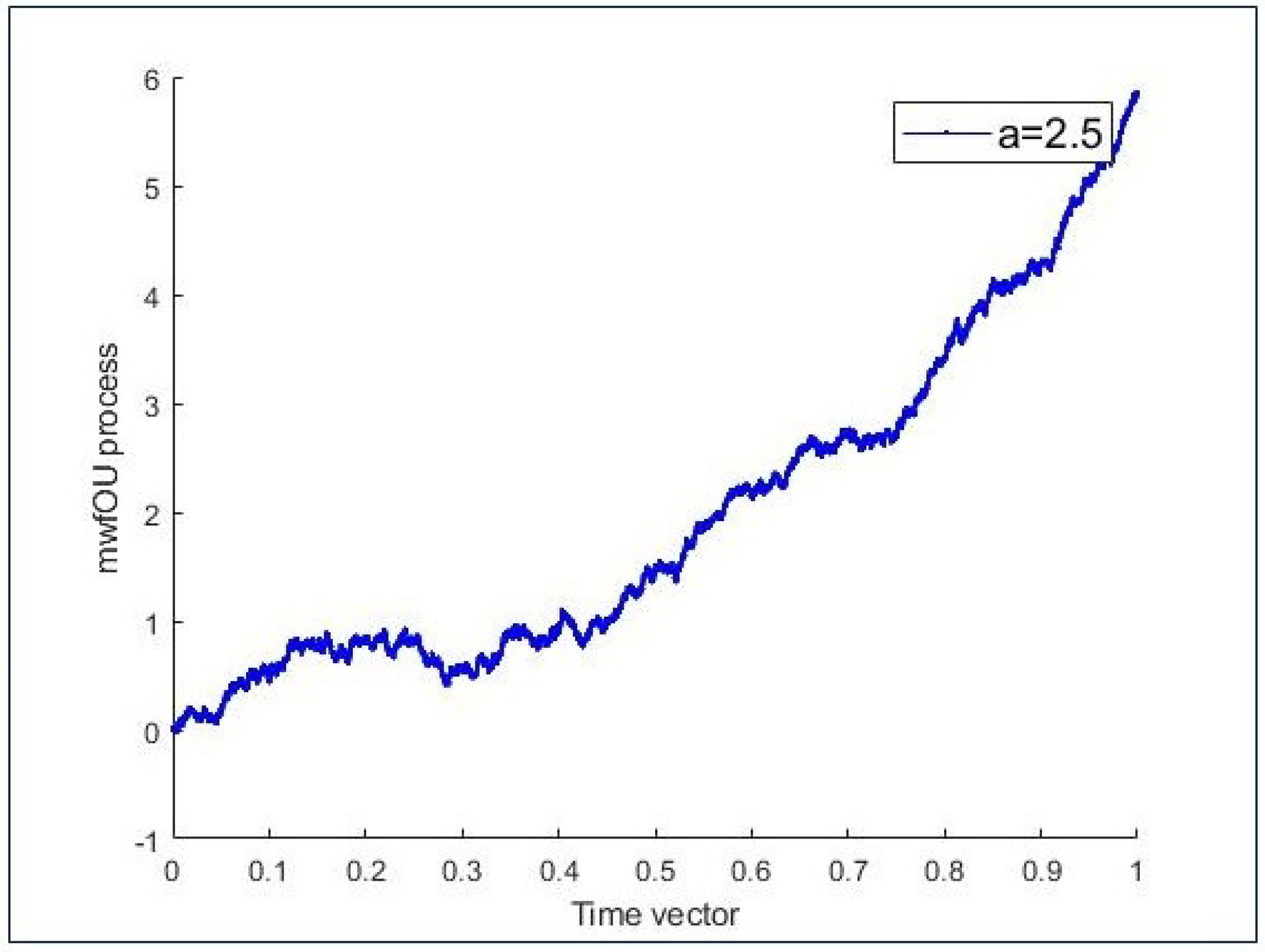
Figure 1. Simulation of sample paths of mwfOU process for large parameter values.
Fractalfract 05 00192 g001
Figure 2. Simulation of sample paths of mwfOU process for small parameter values.
Fractalfract 05 00192 g002
Publisher’s Note: MDPI stays neutral with regard to jurisdictional claims in published maps and institutional affiliations.