Numerical Solution of Fractional Elliptic Problems with Inhomogeneous Boundary Conditions

Abstract

The numerical solution of fractional-order elliptic problems is investigated in bounded domains. According to real-life situations, we assumed inhomogeneous boundary terms, while the underlying equations contain the full-space fractional Laplacian operator. The basis of the convergence analysis for a lower-order boundary element approximation is the theory for the corresponding continuous problem. In particular, we need continuity results for Riesz potentials and the fractional-order extension of the theory for boundary integral equations with the Laplacian operator. Accordingly, the convergence is stated in fractional-order Sobolev norms. The results were confirmed in a numerical experiment.

1. Introduction

The numerical solution of fractional-order diffusion problems has a number of applications to simulate real-world phenomena such as groundwater flows [1], the dynamics of some proteins [2], geophysical electromagnetics [3], or population dynamics [4]. In the last few decades—initiating in the work [5]—different approaches were developed to investigate this important problem. In the space-fractional case, the core of any investigation is the study of the underlying fractional elliptic problem.

Physically, this phenomenon (also called anomalous diffusion) can be recognized by the sublinear dependence of the mean-squared displacement of single particles as a function of time. For further explanations, we refer to the review article [6].

The main difficulty is to deal with these problems on bounded domains. While many different definitions of the full-space fractional Laplacian are equivalent [7], for bounded domains, even in the case of homogeneous boundary conditions, substantially different definitions exist [8]. As in many situations in applied mathematics, the functional analytic point of view leads to the most adequate model [9]. Since the discretization of the fractional Laplacian results in a dense matrix in any case, the numerical treatment of the related problems needs special techniques; see [10,11,12]. At the same time, based on the nonlocal property of the fractional Laplacian, the zero-order extension to ${\mathbb{R}}^d$ also makes sense. The corresponding numerical approximation—containing integrals on ${\mathbb{R}}^d$—also needs special care [13]. For a review paper on nonlocal models and their numerical approximations with further literature, we refer to [14].

The real challenge, however, is the incorporation of inhomogeneous boundary conditions. Indeed, it seems to be hard to model this nonlocal phenomenon if we only have boundary data. Namely, for the computation of the full-space fractional Laplacian, we would need the values of the underlying function on the whole space ${\mathbb{R}}^d$.

A few attempts were made to resolve this problem in the framework of the conventional PDEs, starting from the work [15], which were summarized in detail in [16]. An alternative approach can be found in [17]. It turns out that the boundary integral form of these problems offers a meaningful alternative.

This idea was initiated in [18] and completed with all possible cases in [19]. This can also constitute the basis of the present study, where boundary integral elements are used.

Accordingly, the objective of this work is to set the theoretical basis of the boundary element method for fractional-order elliptic problems, which can successfully deal with inhomogeneous boundary conditions. Extending the classical approach for the second-order elliptic case, we state the convergence properties of this approach and present a series of numerical experiments.

2. Materials and Methods

In practice, the unknown function u has to be computed on a bounded domain $\Omega \subset {\mathbb{R}}^d$ with $d=2,3$, which is assumed to have Lipschitz boundary. The convergence results are given in terms of fractional Sobolev norms. For the full space ${\mathbb{R}}^d$, these are usually defined using the Fourier transform $\mathcal{F}$ on the vector space:

$$H^s\left({\mathbb{R}}^d\right)=\{v\in L_2\left({\mathbb{R}}^d\right):{\int }_{{\mathbb{R}}^d}{(1+|\mathbf{r}|}^2{)}^s{\left|\mathcal{F}v\right|}^2\left(\mathbf{r}\right)\mathrm{d}\mathbf{r}<\infty \}$$

as follows:

$${\parallel v\parallel }_{H^s\left({\mathbb{R}}^d\right)}^2={\int }_{{\mathbb{R}}^d}{(1+|\mathbf{r}|}^2{)}^s{\left|\mathcal{F}v\right|}^2\left(\mathbf{r}\right)\mathrm{d}\mathbf{r}.$$

(1)

Here, s is an arbitrary positive index. Using this, one can define the local version with:

$${\parallel v\parallel }_{H^s(\Omega )}=\underset{\tilde{v}\in H^s\left({\mathbb{R}}^d\right)}{inf}\{\parallel \tilde{v}{\parallel }_{H^s\left({\mathbb{R}}^d\right)}:\tilde{v}{|}_{\Omega }=v\}.$$

(2)

For the details, we refer to the monograph [20].

In the error analysis, we considered a tessellation:

$${\overline{\Gamma }}_1\cup {\overline{\Gamma }}_2\cup \cdots \cup {\overline{\Gamma }}_N=\Gamma =\partial \Omega$$

of the boundary such that the surface subdomains ${\left\{{\Gamma }_j\right\}}_{j=1}^N$ are disjoint open Lipschitz domains, which were assumed to be a $C^1$-diffeomorphic map of a convex polygon for $d=3$ or a bounded interval for $d=2$.

We also need an estimate concerning piecewise Sobolev spaces.

Lemma 1

([21], p. 37). For the above tessellation and any $v\in H^s(\partial \Omega )$ with $s>0$, we have the estimate:

$${\parallel v\parallel }_{H^{-s}(\partial \Omega )}\le \sum _{j=1}^N{\parallel v_{|{\Gamma }_j}\parallel }_{H^{-s}\left({\Gamma }_j\right)}.$$

For stating the well-posedness of the continuous problem, we also need the Sobolev space:

$${\dot{H}}^s\left({\mathbb{R}}^d\right)=\left\{u\in L_{2,\mathrm{loc}}(\Omega ):{\int }_{{\mathbb{R}}^d}{\left|\mathbf{r}\right|}^{2s}{\left|\mathcal{F}u\right|}^2\left(\mathbf{r}\right)\mathrm{d}\mathbf{r}<\infty \right\}$$

with the corresponding norm.

The full-space fractional Laplacian operator [7] can be defined pointwise as:

$$-{(-{\Delta }_{{\mathbb{R}}^d})}^{\alpha }u\left(\mathbf{x}\right)=\underset{r\to 0^{+}}{lim}\frac{2^{2\alpha }\Gamma (\frac{d}{2}+\alpha )}{{\pi }^{\frac{d}{2}}\Gamma (-\alpha )}{\int }_{B{(\mathbf{0},r)}^C}\frac{u(\mathbf{x}+\mathbf{z})-u\left(\mathbf{x}\right)}{{\left|\mathbf{z}\right|}^{d+2\alpha }}\mathrm{d}\mathbf{z},$$

(3)

where $B{(\mathbf{x},r)}^C={\mathbb{R}}^d\backslash B(\mathbf{x},r)$. One can also define its weak form as the function ${(-{\Delta }_{{\mathbb{R}}^d})}^{\alpha }$ for which:

$${\int }_{{\mathbb{R}}^d}v{(-{\Delta }_{{\mathbb{R}}^d})}^{\alpha }u={\int }_{{\mathbb{R}}^d}u{(-{\Delta }_{{\mathbb{R}}^d})}^{\alpha }v$$

is satisfied for all $v\in C_0^{\infty }\left({\mathbb{R}}^d\right)$.

The success of the boundary integral methods hinges on the existence of the fundamental solution ${\varphi }_{\alpha }$ of ${(-{\Delta }_{{\mathbb{R}}^d})}^{\alpha }$, which is given with:

$${\varphi }_{\alpha }={\mathcal{F}}^{-1}\frac{1}{{\left|\mathrm{Id}\right|}^{2\alpha }}=2^{\alpha -\frac{d}{2}}\frac{\Gamma \left(\frac{\alpha }{2}\right)}{\Gamma \left(\frac{d-\alpha }{2}\right)}{\left|\mathrm{Id}\right|}^{2\alpha -d}.$$

(4)

We also used the concept of the trace operator $\gamma$, which for a bounded Lipschitz domain $\Omega$ is continuous as:

$$\gamma :H^s(\Omega )\to H^{s-\frac{1}{2}}(\partial \Omega )$$

(5)

for $s\in (\frac{1}{2},\frac{3}{2})$; see [22], Theorem 3.38.

We applied the conventional notation ${⟨·,·⟩}_{-\beta ,\beta }$ for the duality pairing between $H^{-\beta }(\partial \Omega )$ and $H^{\beta }(\partial \Omega )$ with some positive exponent $\beta$.

To streamline the presentation, we use the notation ${\parallel ·\parallel }_{s,\Omega }$ for the Sobolev norm in the space $H^s(\Omega )$ and similarly with $\Gamma$. Furthermore, in the estimates, the relation ≲ was used if the left-hand side can be estimated with a domain-dependent constant times the right-hand side.

The main problem in practice is the numerical solution of the elliptic boundary value problem:

$$\left\{\begin{array}{c}-{(-\Delta )}^{\alpha }u\left(\mathbf{x}\right)=f\left(\mathbf{x}\right)\mathbf{x}\in \Omega \hfill \\ u\left(\mathbf{x}\right)=g\left(\mathbf{x}\right)\mathbf{x}\in \partial \Omega ,\hfill \end{array}\right.$$

where $f,g$ are given real functions. At this stage, the differential operator ${(-\Delta )}^{\alpha }$ is not yet defined. In any case, it should be linear, such that u can be given as $u=u_1+u_2$, where:

$$\left\{\begin{array}{c}-{(-\Delta )}^{\alpha }{u}_1\left(\mathbf{x}\right)=f\left(\mathbf{x}\right)\mathbf{x}\in \Omega \hfill \\ u_1\left(\mathbf{x}\right)=0\mathbf{x}\in \partial \Omega \hfill \end{array}\right.$$

(6)

and:

$$\left\{\begin{array}{c}-{(-\Delta )}^{\alpha }{u}_2\left(\mathbf{x}\right)=0\mathbf{x}\in \Omega \hfill \\ u_2\left(\mathbf{x}\right)=g\left(\mathbf{x}\right)\mathbf{x}\in \partial \Omega .\hfill \end{array}\right.$$

(7)

The problem in (6) is equipped with homogeneous boundary conditions, which has already been studied by many authors, as mentioned in Section 1. Therefore, in this study, we investigate the numerical solution of the problem:

$$\left\{\begin{array}{c}-{(-{\Delta }_{{\mathbb{R}}^d})}^{\alpha }\tilde{u}\left(\mathbf{x}\right)=0\mathbf{x}\in {(\partial \Omega )}^C\hfill \\ \tilde{u}\left(\mathbf{x}\right)=g\left(\mathbf{x}\right)\mathbf{x}\in \partial \Omega \hfill \\ |\tilde{u}{\left(\mathbf{x}\right)|\lesssim |\mathbf{x}|}^{2\alpha -d}\mathbf{x}\in B{(\mathbf{0},1)}^C,\hfill \end{array}\right.$$

(8)

corresponding to (7), using boundary element approximation.

The result in [19] ensures the well-posedness of (8) as follows.

Theorem 1

([18,19]). For any bounded Lipschitz domain $\Omega \subset {\mathbb{R}}^d$ with $d\ge 3$ and $\alpha \in (\frac{1}{2},1)$, or with $d=2$ and $\alpha \in (\frac{1}{2},\frac{3}{4}]$ and $g\in H^{\alpha -\frac{1}{2}}(\partial \Omega )$, the problem in (8) has a unique weak solution $\tilde{u}\in {\dot{H}}^{\alpha }\left({\mathbb{R}}^d\right)$.

The main building block of the proof is the analysis of the surface potential corresponding to ${\varphi }_{\alpha }$ on $\partial \Omega$, which is given for any $\mathbf{x}\in {\mathbb{R}}^d$ with:

$$S_{\alpha }\left(u\right)\left(\mathbf{x}\right)={\int }_{\partial \Omega }{\varphi }_{\alpha }(\mathbf{x}-\mathbf{y})u\left(\mathbf{y}\right)\mathrm{d}{S}_{\mathbf{y}},$$

(9)

where ${\varphi }_{\alpha }:{\mathbb{R}}^d\backslash \mathbf{0}\to \mathbb{R}$ is given in (4). In particular, the following result was established in [19].

Theorem 2

([19]). For any indices $s,\alpha$ satisfying the assumptions in Theorem 1 and $2\alpha -s\in (\frac{1}{2},\frac{3}{2})$, the mapping $S_{\alpha }$ defines a continuous linear operator between $H^{s-2\alpha +\frac{1}{2}}(\partial \Omega )$ and $H^s(\Omega )$, i.e., for all $\psi \in H^{s-2\alpha +\frac{1}{2}}(\partial \Omega )$, we have:

$$\parallel S_{\alpha }{\left(\psi \right)\parallel }_s\lesssim {\parallel \psi \parallel }_{s-2\alpha +\frac{1}{2},\partial \Omega }.$$

(10)

Moreover, the map $\gamma S_{\alpha }$ is a coercive operator between $H^{1/2-\alpha }(\partial \Omega )$ and $H^{\alpha -1/2}(\partial \Omega )$ in the sense that:

$${⟨u,\gamma S_{\alpha }u⟩}_{\frac{1}{2}-\alpha ,\alpha -\frac{1}{2}}={\int }_{\partial \Omega }\left(S_{\alpha }u\right)\left(\mathbf{x}\right)u\left(\mathbf{x}\right)\mathrm{d}{S}_{\mathbf{x}}\gtrsim {\parallel u\parallel }_{1/2-\alpha ,\partial \Omega }^2.$$

(11)

3. Results

3.1. Error Analysis

The surface potential $S_{\alpha }$ allows us to reformulate the problem in (8). We want to find the unique solution to the equation:

$$\gamma S_{\alpha }\left(u\right)=g.$$

(12)

To approximate the solution of Equation (12), first, we introduced the trial space for a Galerkin approach. In all cases, the subscript h denotes a parameter corresponding to the discretization.

We made use of the trial space:

$$S_h^0(\Gamma )=\{w\in L^2(\Gamma ):w_{|{\Gamma }_j}\in {\mathcal{P}}^0\forall j=1,2,\cdots ,N\},$$

i.e., $S_h^0(\Gamma )$ is piecewise constant with respect to the surface mesh. This trial space fulfills the relation $S_h^0(\Gamma )\subset H^{1/2-\alpha }(\Gamma )$. A suitable basis of $S_h^0(\Gamma )$ is given by ${\left\{{\phi }_j\right\}}_{j=1}^N$, where:

$${\phi }_j\left(x\right)=\left\{\begin{array}{c}1\mathrm{if}x\in {\Gamma }_j,\hfill \\ 0\mathrm{otherwise}.\hfill \end{array}\right.$$

Now, we can apply the Galerkin formulation:

$$\mathrm{find}{u}_h\in S_h^0(\Gamma ):{⟨v_h,\gamma S_{\alpha }\left(u_h\right)⟩}_{\frac{1}{2}-\alpha ,\alpha -\frac{1}{2}}={⟨v_h,g⟩}_{\frac{1}{2}-\alpha ,\alpha -\frac{1}{2}}\forall v_h\in S_h^0(\Gamma ),$$

(13)

which implies the Galerkin orthogonality relation:

$${⟨v_h,\gamma S_{\alpha }(u-u_h)⟩}_{\frac{1}{2}-\alpha ,\alpha -\frac{1}{2}}=0\forall v_h\in S_h^0(\Gamma ).$$

(14)

The starting point of the analysis is to state the quasi-optimality of any Galerkin method as follows.

Lemma 2

(Céa-lemma). For the Galerkin solution $u_h$ of Equation (13), we have:

$$\parallel u-u_h{\parallel }_{\frac{1}{2}-\alpha ,\partial \Omega }\lesssim \underset{w_h\in S_h^0(\partial \Omega )}{inf}{\parallel u-w_h\parallel }_{\frac{1}{2}-\alpha ,\partial \Omega }.$$

(15)

Proof. 

Using the coercivity in (11), the orthogonality relation in (14), and finally, the continuity in (10), we obtain that for any $w_h\in S_h^0$, the following estimation is valid:

$$\begin{array}{cc}\hfill \parallel u-u_h{\parallel }_{\frac{1}{2}-\alpha ,\partial \Omega }^2& \lesssim {⟨u-u_h,\gamma S_{\alpha }(u-u_h)⟩}_{\frac{1}{2}-\alpha ,\alpha -\frac{1}{2}}\hfill \\ \hfill & ={⟨u-w_h,\gamma S_{\alpha }(u-u_h)⟩}_{\frac{1}{2}-\alpha ,\alpha -\frac{1}{2}}\hfill \\ \hfill & \le \parallel u-w_h{\parallel }_{\frac{1}{2}-\alpha ,\partial \Omega }{\parallel \gamma S_{\alpha }(u-u_h)\parallel }_{\alpha -\frac{1}{2},\partial \Omega }\hfill \\ \hfill & \lesssim \parallel u-w_h{\parallel }_{\frac{1}{2}-\alpha ,\partial \Omega }{\parallel u-u_h\parallel }_{\frac{1}{2}-\alpha ,\partial \Omega }.\hfill \end{array}$$

Dividing both sides of the equation by $\parallel u-u_h{\parallel }_{\frac{1}{2}-\alpha ,\partial \Omega }$, we obtain:

$$\parallel u-u_h{\parallel }_{\frac{1}{2}-\alpha ,\partial \Omega }\lesssim {\parallel u-w_h\parallel }_{\frac{1}{2}-\alpha ,\partial \Omega },$$

which also implies:

$$\parallel u-u_h{\parallel }_{\frac{1}{2}-\alpha ,\partial \Omega }\lesssim \underset{w_h\in S_h^0(\partial \Omega )}{inf}{\parallel u-w_h\parallel }_{\frac{1}{2}-\alpha ,\partial \Omega },$$

as stated in the lemma.    □

We can verify the stability of the above Galerkin method by applying (11) for $u=u_h$:

$$\parallel u_h{\parallel }_{\frac{1}{2}-\alpha }^2\lesssim {⟨u_h,\gamma S_{\alpha }{u}_h⟩}_{\frac{1}{2}-\alpha ,\alpha -\frac{1}{2}}={⟨u_h,g⟩}_{\frac{1}{2}-\alpha ,\alpha -\frac{1}{2}}\le \parallel u_h{\parallel }_{\frac{1}{2}-\alpha }{\parallel g\parallel }_{\alpha -\frac{1}{2}}.$$

Dividing both sides by $\parallel u_h{\parallel }_{\frac{1}{2}-\alpha }$, we obtain stability on the boundary:

$$\parallel u_h{\parallel }_{\frac{1}{2}-\alpha }\lesssim {\parallel g\parallel }_{\alpha -\frac{1}{2}}.$$

Now, applying (10), we finally obtain stability for the reconstructed solution as:

$$\parallel {\tilde{u}}_h{\parallel }_{\alpha }=\parallel S_{\alpha }\left(u_h\right){\parallel }_{\alpha }\lesssim \parallel u_h{\parallel }_{\frac{1}{2}-\alpha }\lesssim {\parallel g\parallel }_{\alpha -\frac{1}{2}.}$$

We need the approximation property of $S_h^0$ on each surface subdomain ${\Gamma }_j$ separately. For this, we introduced the projection operator $Q_h^j:L^2\left({\Gamma }_j\right)\to S_h^0\left({\Gamma }_j\right)$ defined by:

$${(Q_h^{j}v,v_h)}_{L^2\left({\Gamma }_j\right)}={(v,v_h)}_{L^2\left({\Gamma }_j\right)}\forall v_h\in S_h^0\left({\Gamma }_j\right).$$

An appropriate statement can be found in [21], Theorem 10.14, on p. 237, which was adapted to our notation using $1/2-\alpha :=\sigma$.

Lemma 3.

For any $\alpha \in [\frac{1}{2},\frac{3}{2}]$ and $s\in [1/2-\alpha ,1]$, the projection operator $Q_h^j$ has the following approximation property:

$$\begin{array}{c}\hfill \underset{w_h\in S_h^0\left({\Gamma }_j\right)}{inf}\parallel u-w_h{\parallel }_{1/2-\alpha ,{\Gamma }_j}=\parallel u-Q_h^j{u\parallel }_{1/2-\alpha ,{\Gamma }_j}\lesssim h^{s-(1/2-\alpha )}{\parallel u\parallel }_{s,{\Gamma }_j}.\end{array}$$

(16)

Note that the condition in Theorem 1 and in Theorem 2 for $\alpha$ is also sufficient in Lemma 3.

We can now prove the following error estimate for the boundary element approximation.

Theorem 3.

Assume that $g\in H^{\alpha -\frac{1}{2}}(\partial \Omega )$ and $s\in [1/2-\alpha ,1]$. Let u be the solution of (12) and $u_h$ be the solution of (13). Then, for every $j\in \{1,2,\cdots ,N\}$, we have:

$$\parallel u-u_h{\parallel }_{1/2-\alpha ,{\Gamma }_j}\lesssim h^{s-(1/2-\alpha )}{\parallel u\parallel }_{s,{\Gamma }_j}.$$

(17)

Proof. 

Using (15) and (16), we obtain:

$$\parallel u-u_h{\parallel }_{1/2-\alpha ,{\Gamma }_j}\lesssim \underset{w_h\in S_h^0(\partial \Omega )}{inf}\parallel u-w_h{\parallel }_{\frac{1}{2}-\alpha ,\partial \Omega }\lesssim h^{s-(1/2-\alpha )}{\parallel u\parallel }_{s,{\Gamma }_j},$$

(18)

as stated in the theorem.    □

Using this, we finally state an error estimate for the solution of (8).

Theorem 4.

Assume that the conditions in Theorems 1 and 2 are satisfied. Then, we have the error estimation:

$$\parallel \tilde{u}-{\tilde{u}}_h{\parallel }_{\alpha ,{\mathbb{R}}^d}\lesssim \sum _{{\Gamma }_j\in \partial \Omega }{h}^{s-(1/2-\alpha )}{\parallel u\parallel }_{s,{\Gamma }_j}$$

(19)

for the boundary element based approximation ${\tilde{u}}_h$ of the solution of (8).

Proof. 

We first note that ${\tilde{u}}_h$ is obtained via reconstruction by applying the surface potential $S_{\alpha }$ as follows:

$${\tilde{u}}_h\left(\mathbf{x}\right)={\int }_{\Gamma }{\varphi }_{\alpha }(\mathbf{x}-\mathbf{y})u_h\left(\mathbf{y}\right)d{S}_{\mathbf{y}}=S_{\alpha }\left(u_h\right)\left(\mathbf{x}\right).$$

(20)

Applying the same for the analytic solution u of (8), we obtain the following expansion for the error of the reconstructed solution:

$$\tilde{u}\left(\mathbf{x}\right)-{\tilde{u}}_h\left(\mathbf{x}\right)=S_{\alpha }\left(u\right)\left(\mathbf{x}\right)-S_{\alpha }\left(u_h\right)\left(\mathbf{x}\right)=S_{\alpha }(u-u_h)\left(\mathbf{x}\right).$$

Using this, then applying (10) for $u-u_h$ in Theorem 2, using Lemma 1, and finally, the estimation (17), we obtain:

$$\begin{array}{cc}\hfill \parallel \tilde{u}-{\tilde{u}}_h{\parallel }_{\alpha ,{\mathbb{R}}^n}& =\parallel S_{\alpha }(u-u_h){\parallel }_{\alpha ,{\mathbb{R}}^d}\lesssim {\parallel u-u_h\parallel }_{1/2-\alpha ,\partial \Omega }\hfill \\ \hfill & \lesssim \sum _{{\Gamma }_j\in \partial \Omega }\parallel u-u_h{\parallel }_{\frac{1}{2}-\alpha ,{\Gamma }_j}\lesssim \sum _{{\Gamma }_j\in \partial \Omega }{h}^{s-(1/2-\alpha )}{\parallel u\parallel }_{s,{\Gamma }_j},\hfill \end{array}$$

as stated in the theorem.    □

3.2. Numerical Experiments

Let us take the domain $\Omega \in {\mathbb{R}}^2$ to be the unit disk. We investigated the model problem:

$$\left\{\begin{array}{c}-{(-\Delta )}^{\alpha }\tilde{u}\left(\mathbf{x}\right)=0\left|\mathbf{x}\right|\ne 1\hfill \\ \tilde{u}\left(\mathbf{x}\right)=g\left(\mathbf{x}\right)\left|\mathbf{x}\right|=1\hfill \\ |\tilde{u}{\left(\mathbf{x}\right)|\lesssim |\mathbf{x}|}^{2\alpha -2}\left|\mathbf{x}\right|>1,\hfill \end{array}\right.$$

(21)

for different values of $\alpha \in (\frac{1}{2},\frac{3}{4}]$ according to Theorem 1, where the analytic solution $\tilde{u}$ is given with:

$$\tilde{u}\left(\mathbf{x}\right)={\int }_{\left|\mathbf{y}\right|=1}{\varphi }_{\alpha }(\mathbf{x}-\mathbf{y})f\left(\mathbf{y}\right)\mathrm{d}\mathbf{y},$$

(22)

where:

$$f\left(\mathbf{y}\right)=f(x,y)=x^2+sin\left(10y\right)$$

(23)

and:

$$g\left(\mathbf{x}\right)=\tilde{u}\left(\mathbf{x}\right)\left|\mathbf{x}\right|=1.$$

(24)

For the experimental error analysis, we first computed the analytic solution $\tilde{u}$ inside the domain given in (22) using f in (23). For this, a quadrature was applied on the unit circle with 10,000 equidistributed points. In this way, even the analytic solution should be approximated for the experimental error analysis.

We also computed the boundary condition g for our model problem. For this, we applied the built-in MATLAB algorithm integral, which is suitable to compute the singular integrals on the boundary. In our experiment, we solved Equation (21) numerically for different values of $\alpha =0.75,0.7,0.65$. In the cases where $\alpha \le 0.6$, the built-in quadrature integral cannot compute the boundary conditions accurately enough, so we omitted these cases.

Note that in a real-life problem, usually, the boundary condition g is given (instead of the function f), so the method can still be used.

Then, we applied the boundary element method in (13) to compute the approximation $u_h$ using the boundary data g in (24). To compute the terms in the corresponding discrete variational formulation (13), we need to compute the entries of the matrix $S_h$ given by:

$${\left[S_h\right]}_{ij}:=⟨{\phi }_j,\gamma S_{\alpha }{\phi }_i⟩={\int }_{{\Gamma }_j}{\int }_{{\Gamma }_i}{\varphi }_{\alpha }(\mathbf{x}-\mathbf{y})\mathrm{d}\mathbf{y}\mathrm{d}\mathbf{x}i,j=1,2,\cdots ,N.$$

To obtain the diagonal elements here, one needs to take special care, as a conventional three-point Gauss quadrature does not deliver sufficient accuracy. Instead, we applied the built-in MATLAB subroutine integral2, which can handle singularities in the two-dimensional integrand.

Completing the linear system corresponding to (13), we computed the entries in its right-hand side $g_h$ as:

$${\left[g_h\right]}_j:=⟨{\phi }_j,g⟩={\int }_{{\Gamma }_j}g\left(\mathbf{x}\right)\mathrm{d}\mathbf{x}j=1,2,\cdots ,N,$$

(25)

which were approximated using a simple midpoint quadrature.

Finally, we reconstructed ${\tilde{u}}_h$ according to (20), which was the most technical and time-consuming part of the computation. This was performed in each point of a grid in the unit disk. This grid size was approximately the same as the one on the boundary. To approximate the integrals in (20) for a fixed $\mathbf{x}\notin \Gamma$, we applied a midpoint approximation on the boundary using the same mesh as for the solution of (13).

In the boundary element method, we used different partitions of the unit circle, into $N=8,16,32,64,128,256$, and 512 uniform parts. In each case, the computational error was calculated in the $L_2(\Omega )$-norm. After the consecutive refinements, we estimated the corresponding convergence rate, which is called the rate in the tables. Note that in (19), the error estimation is given in $H^{\alpha }(\Omega )$-norm, so we expect the order of convergence to be higher in the $L_2(\Omega )$-norm. According to Theorem 4, the expected rate of convergence in the $H^{\alpha }(\Omega )$-norm is $s-(1/2-\alpha )$. Since $\tilde{u}{|}_{\Omega }$ is in $H^1(\Omega )$, this is equal to $1.25$ for $\alpha =0.75$, $1.2$ for $\alpha =0.7$, and $1.15$ for $\alpha =0.65$. In Table 1, Table 2 and Table 3, the results of the experimental error analysis can be found for different exponents.

Table 1. Computational error in $u_h$ of (21) for $\alpha =0.75$ with respect to the $L_2(\Omega )$-norm with the experimental convergence rates.

h	$2\pi /8$	$2\pi /16$	$2\pi /32$	$2\pi /64$	$2\pi /128$	$2\pi /256$	$2\pi /512$
error	$0.252$	$0.107$	$0.037$	$0.012$	$2.7\times {10}^{-3}$	$6.38\times {10}^{-4}$	$2.43\times {10}^{-4}$
rate	−	$1.232$	$1.524$	$1.611$	$2.175$	$2.08$	$1.39$

Table 2. Computational error in $u_h$ of (21) for $\alpha =0.7$ with respect to the $L_2(\Omega )$-norm with the experimental convergence rates.

h	$2\pi /8$	$2\pi /16$	$2\pi /32$	$2\pi /64$	$2\pi /128$	$2\pi /256$	$2\pi /512$
error	$0.396$	$0.173$	$0.064$	$0.022$	$6.9\times {10}^{-3}$	$2\times {10}^{-3}$	$1.5\times {10}^{-3}$
rate	−	$1.192$	$1.435$	$1.576$	$1.642$	$1.818$	$0.339$

Table 3. Computational error in $u_h$ of (21) for $\alpha =0.65$ with respect to the $L_2(\Omega )$-norm with the experimental convergence rates.

h	$2\pi /8$	$2\pi /16$	$2\pi /32$	$2\pi /64$	$2\pi /128$	$2\pi /256$	$2\pi /512$
error	$0.62$	$0.277$	$0.11$	$0.042$	$0.016$	$0.01$	$9.8\times {10}^{-3}$
rate	−	$1.161$	$1.338$	$1.402$	$1.358$	$0.683$	$0.0334$

For relative coarse meshes, in each case, the convergence rate is even faster than expected. At the same time, for a relatively fine mesh, the computation with singular integrals becomes inaccurate, which results in oscillations in $u_h$ and deteriorates the accuracy of the reconstructed approximation ${\tilde{u}}_h$. At the same time, we could achieve a relatively small error of magnitude ${10}^{-4}$ before this phenomenon affected the convergence rate.

We can observe in Table 1 and Table 2 that the convergence rate decreases already for $N=512$ and $N=256$, respectively. In these cases, $\alpha$ is closer to $\frac{1}{2}$, so that the singularities at the computation of the boundary condition become sharper. This makes the applied quadratures less accurate. For the coarser meshes, the convergence rate is still better than the expected rate.

In the case of $\alpha =0.65$, the deterioration of the convergence rates starts earlier at $N=256$. For the coarser meshes, the convergence rate is still better than the expected rate 1.15.

In Figure 1, the numerical solution is shown together with the given boundary data, while in Figure 2, the pointwise error of the numerical solution is presented for $\alpha =0.75$. For $\alpha =0.65$, similar results are shown in Figure 3 and Figure 4.

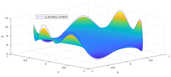
Figure 1. Boundary condition and numerical solution ${\tilde{u}}_h$ of (21) for $\alpha =0.75$ and $N=512$ inside the domain.

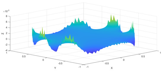
Figure 2. Pointwise error of the numerical solution ${\tilde{u}}_h$ of (21) for $\alpha =0.75$ and $N=512$ inside the boundary. One can observe that most of the error accumulates close to the boundary.

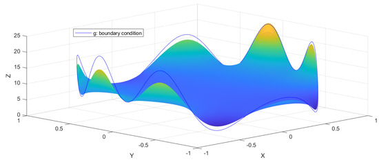
Figure 3. Boundary condition and numerical solution ${\tilde{u}}_h$ of (21) for $\alpha =0.65$ and $N=512$ inside the domain.

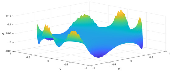
Figure 4. Pointwise error of the numerical solution ${\tilde{u}}_h$ of (21) for $\alpha =0.65$ and $N=512$ inside the boundary. We can observe that the error is significantly larger than in the case of $\alpha =0.75$.

Here, one can already observe some deviation, which is shown in detail in Figure 2, where only the error is presented. At the boundary, indeed, relatively large errors emerge, which were then smoothed out by applying the reconstruction.

4. Discussion

The idea to convert fractional-order elliptic boundary value problems into boundary integral equations leads to well-posed problems with some extra conditions. Furthermore, as the solution is defined everywhere, this corresponds to the nonlocal nature of these problems. Their numerical approximations, which were investigated here, offer also efficient methods. To see this, we recall that for conventional elliptic boundary value problems, boundary element methods lead to dimensional reduction, as well as to full matrices in the resulting linear algebraic problems. In the case of fractional-order problems, however, boundary element methods offer a clear advantage: we have to compute with dense matrices anyway, such that using these methods significantly reduces the computational costs. Moreover, as we have pointed out, in this framework, it is possible to model and simulate the presence of inhomogeneous boundary data. An important future research direction is to extend the well-posedness of the original problem in (8) for $\alpha >\frac{3}{4}$. Furthermore, the application of higher-order elements and the performance of a simple approach, the so-called method of fundamental solutions [23], should be investigated.

References

- Schumer, R.; Benson, D.A.; Meerschaert, M.M.; Wheatcraft, S.W. Eulerian derivation of the fractional advection-dispersion equation. J. Contam. Hydrol. 2001, 48, 69–88. [Google Scholar] [CrossRef]
- Banks, D.S.; Fradin, C. Anomalous Diffusion of Proteins Due to Molecular Crowding. Biophys. J. 2005, 89, 2960–2971. [Google Scholar] [CrossRef] [PubMed]
- Glusa, C.; Antil, H.; D’Elia, M.; Waanders, B.v.; Weiss, C.J. A Fast Solver for the Fractional Helmholtz Equation. SIAM J. Sci. Comput. 2021, 43, 1362–1388. [Google Scholar] [CrossRef]
- Hapca, S.; Crawford, J.W.; Young, I.M. Anomalous diffusion of heterogeneous populations characterized by normal diffusion at the individual level. J. R. Soc. Interface 2009, 30, 111–122. [Google Scholar] [CrossRef] [PubMed]
- Meerschaert, M.M.; Tadjeran, C. Finite difference approximations for fractional advection-dispersion flow equations. J. Comput. Appl. Math. 2004, 172, 65–77. [Google Scholar] [CrossRef]
- Woringer, M.; Darzacq, X. Protein motion in the nucleus: From anomalous diffusion to weak interactions. Biochem. Soc. Trans. 2018, 46, 945–956. [Google Scholar] [CrossRef] [PubMed]
- Kwaśnicki, M. Ten equivalent definitions of the fractional Laplace operator. Fract. Calc. Appl. Anal. 2017, 20, 7–51. [Google Scholar] [CrossRef]
- Servadei, R.; Valdinoci, E. On the spectrum of two different fractional operators. Proc. Roy. Soc. Edinburgh Sect. A 2014, 144, 831–855. [Google Scholar] [CrossRef]
- Izsák, F.; Szekeres, B.J. Models of space-fractional diffusion: A critical review. Appl. Math. Lett. 2017, 71, 38–43. [Google Scholar] [CrossRef]
- Harizanov, S.; Lazarov, R.; Margenov, S.; Marinov, P. Numerical solution of fractional diffusion–reaction problems based on BURA. Comput. Math. Appl. 2020, 80, 316–331. [Google Scholar] [CrossRef]
- Izsák, F.; Szekeres, B.J. Efficient computation of matrix power-vector products: Application for space-fractional diffusion problems. Appl. Math. Lett. 2018, 86, 70–76. [Google Scholar] [CrossRef]
- Vabishchevich, P.N. Numerical solution of time-dependent problems with fractional power elliptic operator. Comput. Method Appl. Math. 2018, 18, 111–128. [Google Scholar] [CrossRef]
- Acosta, G.; Bersetche, F.M.; Borthagaray, J.P. A short FE implementation for a 2d homogeneous Dirichlet problem of a fractional Laplacian. Comput. Math. Appl. 2017, 74, 784–816. [Google Scholar] [CrossRef]
- D’Elia, M.; Du, Q.; Glusa, C.; Gunzburger, M.; Tian, X.; Zhou, Z. Numerical methods for nonlocal and fractional models. Acta Numer. 2020, 29, 1–12. [Google Scholar] [CrossRef]
- Abatangelo, N.; Dupaigne, L. Nonhomogeneous boundary conditions for the spectral fractional Laplacian. Ann. Inst. H. Poincaré Anal. Non Linéaire 2017, 34, 439–467. [Google Scholar] [CrossRef]
- Lischke, A.; Pang, G.; Gulian, M.; Song, F.; Glusa, C.; Zheng, X.; Mao, Z.; Cai, W.; Meerschaert, M.M.; Ainsworth, M.; et al. What is the fractional Laplacian? A comparative review with new results. J. Comput. Phys. 2020, 404, 109009. [Google Scholar] [CrossRef]
- Harizanov, S.; Margenov, S.; Popivanov, N. Spectral Fractional Laplacian with Inhomogeneous Dirichlet Data: Questions, Problems, Solutions. In Advanced Computing in Industrial Mathematics; Georgiev, I., Kostadinov, H., Lilkova, E., Eds.; Springer: Berlin/Heidelberg, Germany, 2018; Volume 961. [Google Scholar] [CrossRef]
- Chang, T. Boundary integral operator for the fractional Laplace equation in a bounded Lipschitz domain. Integr. Equat. Oper. Th. 2012, 72, 345–361. [Google Scholar] [CrossRef][Green Version]
- Izsák, F.; Maros, G. Fractional order elliptic problems with inhomogeneous Dirichlet boundary conditions. Fract. Calc. Appl. Anal. 2020, 23, 378–389. [Google Scholar] [CrossRef]
- Adams, R.; Fournier, J. Sobolev Spaces; Academic Press: Amsterdam, The Netherlands, 2003. [Google Scholar]
- Steinbach, O. Numerical Approximation Methods for Elliptic Boundary Value Problems. Finite and Boundary Elements; Springer: New York, NY, USA, 2008. [Google Scholar]
- McLean, W. Strongly Elliptic Systems and Boundary Integral Equations; Cambridge University Press: Cambridge, UK, 2000. [Google Scholar]
- Mathon, R.; Johnston, R.L. The approximate solution of elliptic boundary-value problems by fundamental solutions. SIAM J. Numer. Anal. 1977, 14, 638–650. [Google Scholar] [CrossRef]
Publisher’s Note: MDPI stays neutral with regard to jurisdictional claims in published maps and institutional affiliations. |
© 2021 by the authors. Licensee MDPI, Basel, Switzerland. This article is an open access article distributed under the terms and conditions of the Creative Commons Attribution (CC BY) license (https://creativecommons.org/licenses/by/4.0/).