Modeling and Application of Fractional-Order Economic Growth Model with Time Delay

Abstract

This paper proposes a fractional-order economic growth model with time delay based on the Solow model to describe the economic growth path and explore the underlying growth factors. It effectively captures memory characteristics in economic operations by adding a time lag to the capital stock. The proposed model is presented in the form of a fractional differential equations system, and the sufficient conditions for the local stability are obtained. In the simulation, the theoretical results are verified and the sensitivity analysis is performed on individual parameters. Based on the proposed model, we predict China’s GDP in the next thirty years through optimization and find medium-to-high-speed growth in the short term. Furthermore, the application results indicate that China is facing the disappearance of demographic dividend and the deceleration of capital accumulation. Therefore, it is urgent for China to increase the total factor productivity (TFP) and transform its economic growth into a trajectory dependent on TFP growth.

1. Introduction

The economic growth model has been extensively followed and studied by economists since the 1950s [1,2,3,4,5]. Analyzing the dynamics and trends of economic growth helps to grasp macroeconomic operation as well as formulate economic policies. As the cornerstone of economic growth theory, the Solow model [6] provided a groundbreaking theoretical framework for subsequent research work on growth. The model explains how capital stock, saving rate, labor force growth rate, capital depreciation, technological progress interact and affect a nation’s total output. Solow’s theory suggests the convergence of economy towards a steady-state path and emphasizes the role of technological progress as the ultimate driving force behind the long-run growth. Despite voluminous works flourishing in the growth literature [7,8], the Solow model is still of great theoretical and empirical significance, attracting enormous professional interest.

The Solow model is actually presented in the form of an ordinary differential equation describing the process of capital accumulation. However, a differential equation of integer order sometimes shows restriction for economic models since amnesia is assumed in all economic agents and memory fading is neglected. Therefore, a fractional derivative is developed to construct economic models due to its nonlocality and memory characteristics in evolutionary processes [9,10]. Compared with the integer-order derivative, the fractional derivative shows global correlation and better description of long-term dependencies and memory in economic data. Numerous experimental results indicate that the fractional-order model is superior to the integer model when dealing with economic dynamic problems [11,12,13].

The fractional derivative, as the main mathematical tool to describe economic dynamics with memory, has been widely studied in modern mathematical economic theory. A review on the history of economic application of fractional dynamics was provided [14]. It divided the economic dynamics evolution into five stages of development. The first two stages were characterized by fractional brownian motion [15]. Long-term dependencies in economic data were pointed out and a time-fractional Black–Scholes equation was proposed. The following two stages were characterized by econophysics and deterministic chaos [16]. Many papers were devoted to the description of power-law memory and fractional-dynamic behaviors in financial processes. The most recent is the mathematical economics stage beginning with the proposal of generalizations of basic economic concepts and classic models. New concepts primarily include economic multiplier with memory, elasticity and marginal value of fractional order etc. [17,18]. Generalizations of classical models include the Harrod–Domar model, Keynes model, Phillips model and Kaldor model etc. [19,20].

Time delay is a common phenomenon widely existing in economic systems. Since most of the economic processes are not only affected by the present state, but also depend largely on related indicators and factors in the past, the delayed mathematical models are more suitable for depicting economic phenomenon. Therefore, some integer-order and fractional-order differential equation models with time delays are proposed in the economic growth literature, and some significant results have been drawn in recent years. A continuous-time neoclassical growth model with time delay was developed to find erratic fluctuations in the capital accumulation process [21]. Shortly thereafter, a generalized Cai model with endogenous labor shift was studied by choosing the delay as the parameter and gave some conditions of stability and bifurcation [22]. Furthermore, the existence and global attractivity of almost periodic solutions were proven for a delayed differential neoclassical growth model [23]. More recently, a generalization of the Keynesian macroeconomic model was proposed with gamma-distributed lag and using fractional differential equations [18].

In terms of economic growth forecasting, empirical researches have been carried out based on different models. A replicable forecasting model was proposed to find an L-shaped GDP growth path in China and predict an annual GDP growth rate close to the 6.5% official target in the next five years [24]. Underlying factors of China’s strong growth were explored using a general framework of cross-country analysis. The forecast results showed a significant decline of China’s potential GDP growth in the coming decade [25]. In terms of fractional calculus, both integer order and fractional order differential equation models were considered to predict the economic growth of the countries in the Group of Twenty [26].

In this paper, we propose an adaptive fractional economic growth model where a time delay is introduced to describe the time lag from capital input to effect. Therefore, our method can effectively capture memory characteristics within economic operations. The traditional Solow model is based on a harsh assumption that the technological progress is completely exogenous, which is not consistent with practical experience. To make up for the gap, we assume in our model that technological progress is endogenous and related to both population and capital. The proposed model is presented in the form of a fractional differential equations system. To explore the steady state of long-term economic growth, we analyze the stability of the equilibrium point and how stability changes when parameters vary. Based on the model, we use China’s economic data to conduct economic forecast and empirical analysis. To achieve this, we first estimate the fractional order of each equation through optimization and analyze the trends of main variables affecting China’s economy. As a meaningful exploration, we compare the delayed fractional model with the integer derivative model and the no delay model, respectively. We also exhibit the impacts of different fractional derivatives and delay parameters on predictions. On this basis, we predict China’s GDP in the next thirty years and analyze its growth potential. The proposed model shows excellent stability properties and predictive results, making it a practicable and attractive approach for analyzing long-term economic growth trends in real applications.

The remainder of this paper is organized as follows. Section 2 provides some definitions and lemmas in fractional differential equation as well as the detailed description of the proposed model. Section 3 shows the main theoretical results on the stability of equilibrium points. Numerical simulation and parameter sensitivity analysis are given in Section 4. Finally, China’s economic growth forecast and analysis in the next thirty years are shown in Section 5.

2. Preliminaries and Model Description

2.1. Definitions and Lemmas

Generally speaking, commonly used definitions of fractional derivatives include Riemann–Liouville derivative definition, Grünwald–Letnikov derivative definition, Caputo derivative definition, etc. Among them, the Caputo derivative definition shows more advantages in actual application, since its initial value has a measurable physical meaning [27,28,29,30]. Moreover, it is widely used to describe economic processes because of its good explanation about the memory characteristics of economic variables [31]. Hence, we adopt the Caputo derivative definition in this paper.

Definition 1

([28]). The Caputo fractional derivative of order q for a function $f\left(t\right)$ is defined as

$${{}_{0}D}_t^{q}f\left(t\right)={\displaystyle \frac{1}{\Gamma (n-q)}}{\int }_0^t{\displaystyle \frac{f^{\left(n\right)}\left(\tau \right)}{{(t-\tau )}^{q-n+1}}}\mathrm{d}\tau ,$$

where $n\in Z^{+},n-1<q<n$, and $\Gamma (·)$ is the Gamma function.

Definition 2

([28]). The Laplace transform of the Caputo fractional derivative is

$$L\{{{}_{0}D}_t^{q}f\left(t\right);s\}=s^{q}F\left(s\right)-\sum _{k=0}^{n-1}{s}^{q-k-1}{f}^{\left(k\right)}\left(0\right),n-1<q<n,$$

where $F\left(s\right)$ is the Laplace transform of $f\left(t\right)$. When $f^{\left(k\right)}\left(0\right)=0,k=1,2,\cdots ,n$, then

$$L\{{{}_{0}D}_t^{q}f\left(t\right);s\}=s^{q}F\left(s\right).$$

We consider the following linear fractional-order system with time delay

$${{}_{0}D}_t^{q}X\left(t\right)=AX\left(t\right)+KX(t-\tau ),$$

(1)

where $A={\left(a_{ij}\right)}_{n\times n},K={\left(k_{ij}\right)}_{n\times n},X\left(t\right)={(x_1\left(t\right),x_2\left(t\right),\cdots ,x_n\left(t\right))}^T,X(t-\tau )={(x_1(t-{\tau }_1),x_2(t-{\tau }_2),\cdots ,x_n(t-{\tau }_n))}^T$.

Taking Laplace transform on both sides of (1), one gets the characteristic matrix [32]

$$\Delta \left(s\right)=\left(\begin{array}{cccc}{s}^q-k_{11}{e}^{-s{\tau }_{11}}-a_{11}& -k_{12}{e}^{-s{\tau }_{12}}-a_{12}& \cdots & -k_{1n}{e}^{-s{\tau }_{1n}}-a_{1n}\\ -k_{21}{e}^{-s{\tau }_{21}}-a_{21}& s^q-k_{22}{e}^{-s{\tau }_{22}}-a_{22}& \cdots & -k_{2n}{e}^{-s{\tau }_{2n}}-a_{2n}\\ ⋮& ⋮& \ddots & ⋮\\ -k_{n1}{e}^{-s{\tau }_{n1}}-a_{n1}& -k_{n2}{e}^{-s{\tau }_{n2}}-a_{n2}& \cdots & s^q-k_{nn}{e}^{-s{\tau }_{nn}}-a_{nn}\end{array}\right).$$

(2)

The stability of system (1) is totally determined by the distribution of the eigenvalues from the characteristic equation det $(\Delta (s\left)\right)=0$. If ${\tau }_{ij}=0$, system (1) can be rewritten as

$${{}_{0}D}_t^{q}X\left(t\right)=AX\left(t\right)+KX\left(t\right)=MX\left(t\right),$$

(3)

where the coefficient matrix $M=A+K$. Then, two useful results about the stability of system (1) are introduced as follows

Lemma 1

([32]). If all the roots of the characteristic equation det $(\Delta (s\left)\right)=0$ for $q\in (0,1)$ have negative real parts, then the zero solution of system (1) is Lyapunov globally asymptotically stable.

Lemma 2

([33]). If $q\in (0,1)$, all the eigenvalues of M satisfy $\left|\arg \left(\lambda \right)\right|>\frac{\pi }{2}$ and the characteristic equation det $(\Delta (s\left)\right)=0$ has no pure imaginary roots for any ${\tau }_{ij}>0,i,j=1,\dots ,n$, then the zero solution of system (1) is Lyapunov asymptotically stable.

2.2. Model Description

The economic growth model based on the Solow model is a three-dimensional system given by [8]

$$\left\{\begin{array}{c}\frac{d{L}_t}{dt}=r(1-L_t/L_m)L_t,\hfill \\ \frac{d{K}_t}{dt}=s{Y}_t-(\delta +g+n)K_t,\hfill \\ \frac{d{A}_t}{dt}=g{A}_t.\hfill \end{array}\right.$$

(4)

Respectively, we explain and improve the above equations as follows.

The working population $L_t$: The fisrt equation is a population growth model based on the logistic approach [34]. $r\in (0,1)$ denotes the natural growth rate of the working population; $L_m>0$ is the maximum number of labor force that can be accommodated under certain natural resources and market scale.

The capital stock $K_t$: The second equation represents the basic Solow model that describes how capital accumulates [6]. Here, $s\in (0,1)$ is the constant saving rate; $\delta \in (0,1)$ is the capital depreciation rate; $g\in (0,1)$ is the growth rate of technology; $n\in (0,1)$ is the population growth rate, and $Y_t,K_t$ denote the gross domestic product and capital stock at time t. Especially, $Y_t$ is defined as Cobb–Douglas production function

$$Y_t=A_t{K}_t^{\alpha }{L}_t^{1-\alpha },$$

(5)

where $A_t$ is an index of the total factor productivity(TFP) and $\alpha \in (0,1)$ is the output elasticity of capital stock.

The total factor productivity (TFP) $A_t$: The third equation determines the growth of TFP. It is typically measured as the “Solow residual”(total output growth less the weighted sum of input growth), and equals the rate of technological progress under the assumption of constant return to scale. An important assumption of the Solow framework is that the technological progress is exogenous and growing at a constant rate g with the form $d{A}_t/dt=g{A}_t$. However, one argument of this assumption is that it simply measures the size of TFP but rarely directly identifies the underlying sources of technological progress [35]. Therefore, recent studies are attempting to search for more possible determinants of TFP growth. As technical talents and capital investment are important factors for technological progress, both human capital stock and physical capital stock contribute to the techonlogical progress rate g [36]. For sake of simplicity, but without losing of generality, we add $K_t$ and $L_t$ into the determinant of techonlogical progress rate g in a linear form as follows

$$g=w{l}_t+h{k}_t+p,$$

(6)

where $l_t={\displaystyle \frac{L_t}{A_t}}$ and $k_t={\displaystyle \frac{L_t}{A_t}}$ is the working population per TFP and the capital stock per TFP, respectively, w and h is the contribution ratio of $l_t$ and $k_t$. Substituting expression (6) into $d{A}_t/dt=g{A}_t$, we obtain

$${\displaystyle \frac{d{A}_t}{dt}}=p{A}_t+w{L}_t+h{K}_t.$$

(7)

As we emphasized in the previous statement, economic processes often show lagging memory characteristics and complex dynamic operations. Therefore, we convert all the integer orders in the above equations into fractional ones to better describe the dynamic behavior of financial and economic system. Especially, for capital stock, physical capital usually cannot play a role in the economic system immediately after installation [37,38]. For example, when an added machine is decided to deploy, it goes through a period of product manufacturing and processing before it can achieve scale effects and increase output. That means there is a time interval between capital input and economic production output. Furthermore, it is a even more self-evident fact that a time interval exists between capital installation and depreciation. Therefore, we introduce a time delay $\tau$ into the capital stock $K_t$ to capture such lagging effect. Thus, the capital stock variable is denoted as $K(t-\tau )$.

Integrating the improvements all above, we obtain the following fractional-order generalization of the Solow-type equation with time delay

$$\left\{\begin{array}{c}{D}_t^{q_1}{L}_t=r(1-L_t/L_m)L_t,\hfill \\ D_t^{q_2}{K}_t=s{A}_t{K}_t^{\alpha }{L}_t^{1-\alpha }-(\delta +g+n)K(t-\tau ),\hfill \\ D_t^{q_3}{A}_t=p{A}_t+w{L}_t+hK(t-\tau ),\hfill \end{array}\right.$$

(8)

where $q_1,q_2,q_3\in (0,1)$ are the fractional orders. In the next stability analysis part, we take $q_1=q_2=q_3=q$.

3. Main Results

Theorem 1.

If $q\in (0,1)$, when $w=0,h<0,0<p<(1-\alpha )(\delta +g+n)$, and $\overline{b}-4y-2\overline{c}+\frac{{\overline{b}}^3-4\overline{b}\overline{c}+8\overline{d}}{\sqrt{8y+{\overline{b}}^2}-4\overline{c}}<0$ or $\overline{b}-4y-2\overline{c}-\frac{{\overline{b}}^3-4\overline{b}\overline{c}+8\overline{d}}{\sqrt{8y+{\overline{b}}^2}-4\overline{c}}<0$, then the positive equilibrium point of system (8) is Lyapunov locally asymptotically stable for any $\tau >0$, where y is any real root of the equation $8y^3-4\overline{c}{y}^2+2(\overline{b}\overline{d}-8\overline{e})y+\overline{e}(4\overline{c}-{\overline{b}}^2)-{\overline{d}}^2=0$, and the coefficients of the equation are denoted as

$$\left\{\begin{array}{c}\overline{b}=-2(\alpha (\delta +g+n)-p)(cosq\pi cos{\displaystyle \frac{q\pi }{2}}+sin(\pm q\pi )sin(\pm {\displaystyle \frac{q\pi }{2}})),\hfill \\ \overline{c}=p^2+2\alpha p(\delta +g+n)(1+cosq\pi )+({\alpha }^2-1){(\delta +g+n)}^2,\hfill \\ \overline{d}=2\alpha p(\delta +g+n)[\alpha (\delta +g+n)-p]cos{\displaystyle \frac{q\pi }{2}},\hfill \\ \overline{e}=p^2{\alpha }^2{(\delta +g+n)}^2.\hfill \end{array}\right.$$

(9)

Proof. 

When $w=0,h<0$, by setting $\tau =0$ and solving the equations

$$\left\{\begin{array}{c}r(1-\overline{L}/L_m)\overline{L}=0,\hfill \\ s\overline{A}{\overline{K}}^{\alpha }{\overline{L}}^{1-\alpha }-(\delta +g+n)\overline{K}=0,\hfill \\ p\overline{A}+h\overline{K}=0,\hfill \end{array}\right.$$

(10)

we obtian the unique positive steady-state solution $(\overline{L},\overline{K},\overline{A})$ of system (8) as

$$\overline{L}=L_m,\overline{K}={\left(-{\displaystyle \frac{p(\delta +g+n)}{sh{L}_m^{(1-\alpha )}}}\right)}^{\frac{1}{\alpha }},\overline{A}=-{\displaystyle \frac{h}{p}}\overline{K}.$$

(11)

when the delay $\tau$ is introduced, the equilibrium point keeps the same and, therefore, we can take the local coordinates

$$\widetilde{L_t}=L_t-\overline{L},\widetilde{K_t}=K_t-\overline{K},\widetilde{A_t}=A_t-\overline{A},$$

and centre the system’s singular point at the origin. If we have $X\left(t\right)=(\widetilde{L_t},\widetilde{K_t},\widetilde{A_t})$, the linear centralized system (8) can be written in the following vector form

$$D_t^{q}X\left(t\right)=AX\left(t\right)+\overline{B}X\left(t\right)+\overline{C}X\left(t\right).$$

(12)

where

$$A=\left(\begin{array}{ccc}r& 0& 0\\ 0& 0& 0\\ 0& 0& p\end{array}\right),$$

and $\overline{B},\overline{C}$ denote the Jacobian matrix

$$\overline{B}=\left(\begin{array}{ccc}{b}_{11}& 0& 0\\ b_{21}& b_{22}& b_{23}\\ 0& 0& 0\end{array}\right)=\left(\begin{array}{ccc}-2r& 0& 0\\ (1-\alpha )s\overline{A}{\overline{K}}^{\alpha }{\overline{L}}^{-\alpha }& \alpha s\overline{A}{\overline{K}}^{\alpha -1}{\overline{L}}^{1-\alpha }& s{\overline{K}}^{\alpha }{\overline{L}}^{1-\alpha }\\ 0& 0& 0\end{array}\right)$$

(13)

$$=\left(\begin{array}{ccc}-2r& 0& 0\\ (1-\alpha )(\delta +g+n){\left(-{\displaystyle \frac{p(\delta +g+n)}{sh{L}_m}}\right)}^{\frac{1}{\alpha }}& \alpha (\delta +g+n)& -{\displaystyle \frac{p}{h}}(\delta +g+n)\\ 0& 0& 0\end{array}\right),$$

$$\overline{C}=\left(\begin{array}{ccc}0& 0& 0\\ 0& c_{22}& 0\\ 0& h& 0\end{array}\right)=\left(\begin{array}{ccc}0& 0& 0\\ 0& -(\delta +g+n)& 0\\ 0& h& 0\end{array}\right).$$

(14)

 □

According to matrix (2), applying Laplace transform on both sides of system (12), one has the following characteristic matrix

$$\Delta \left(s\right)=\left(\begin{array}{ccc}{s}^q+r& 0& 0\\ -b_{21}& s^q-c_{22}{e}^{-s\tau }-b_{22}& -b_{23}\\ 0& -h{e}^{-s\tau }& s^q-p\end{array}\right).$$

(15)

Then, it follows that the characteristic equation $det(\Delta (s\left)\right)=0$ is given as

$$(s^q+r)(s^{2q}-a{s}^q-c_{22}{s}^q{e}^{-s\tau }+b{e}^{-s\tau }+p{b}_{22})=0.$$

(16)

Next, it will be verified that the characteristic Equation (16) has no pure imaginary roots for any $\tau >0$. The fact is testified by contradiction. It is obvious that there are no pure imaginary roots in equation $s^q+r=0$ when $r>0$. Therefore, we consider the equation

$$s^{2q}-a{s}^q-c_{22}{s}^q{e}^{-s\tau }+b{e}^{-s\tau }+p{b}_{22}=0.$$

(17)

Suppose that $s^{*}$ is one of the pure root imaginary of Equation (17) and has the form $s^{*}=wi=\left|w\right|(cos\left(\frac{\pi }{2}\right)+isin(\pm \frac{\pi }{2}))$, where w is a positive real number. The substitution of $s^{*}$ into Equation (17) gives:

$$\begin{array}{c}{\left|w\right|}^{2q}(cosq\pi +isin(\pm q\pi ))-a{\left|w\right|}^q(cos{\displaystyle \frac{q\pi }{2}}+isin(\pm {\displaystyle \frac{q\pi }{2}}))\hfill \\ -c_{22}{\left|w\right|}^q(cos{\displaystyle \frac{q\pi }{2}}+isin(\pm {\displaystyle \frac{q\pi }{2}}))(cosw\tau -isinw\tau )\hfill \\ +b(cosw\tau -isinw\tau )+p{b}_{22}=0.\hfill \end{array}$$

(18)

Separating its real part and imaginary part, we obtain

$${\left|w\right|}^{2q}cosq\pi -{a\left|w\right|}^{q}cos{\displaystyle \frac{q\pi }{2}}+p{b}_{22}=(c_{22}{\left|w\right|}^{q}cos{\displaystyle \frac{q\pi }{2}}-b)cosw\tau +c_{22}{\left|w\right|}^{q}sin(\pm {\displaystyle \frac{q\pi }{2}})sinw\tau ,$$

(19)

and

$${\left|w\right|}^{2q}sin(\pm q\pi )-{a\left|w\right|}^{q}sin(\pm {\displaystyle \frac{q\pi }{2}})=(b-c_{22}{\left|w\right|}^{q}cos{\displaystyle \frac{q\pi }{2}})sinw\tau +c_{22}{\left|w\right|}^{q}sin(\pm {\displaystyle \frac{q\pi }{2}})cosw\tau .$$

(20)

We denote that

$$\left\{\begin{array}{c}{\beta }_1={\left|w\right|}^{2q}cosq\pi -a{\left|w\right|}^{q}cos{\displaystyle \frac{q\pi }{2}}+p{b}_{22},\hfill \\ {\beta }_2={\left|w\right|}^{2q}sin(\pm q\pi )-a{\left|w\right|}^{q}sin(\pm {\displaystyle \frac{q\pi }{2}}),\hfill \\ {\rho }_1=c_{22}{\left|w\right|}^{q}cos{\displaystyle \frac{q\pi }{2}}-b,\hfill \\ {\rho }_2=c_{22}{\left|w\right|}^{q}sin(\pm {\displaystyle \frac{q\pi }{2}}).\hfill \end{array}\right.$$

(21)

Thus, Equations (19) and (20) can be changed into

$$\left\{\begin{array}{c}{\rho }_{1}cosw\tau +{\rho }_{2}sinw\tau ={\beta }_1,\hfill \\ -{\rho }_{1}sinw\tau +{\rho }_{2}cosw\tau ={\beta }_2.\hfill \end{array}\right.$$

(22)

We square both sides of Equation (22) and add them together

$${\rho }_1^2+{\rho }_2^2={\beta }_1^2+{\beta }_2^2.$$

(23)

Substituting expression (21) into Equation (23), we obtain

$${\left|w\right|}^{4q}+\overline{b}{\left|w\right|}^{3q}+\overline{c}{\left|w\right|}^{2q}+\overline{d}{\left|w\right|}^q+\overline{e}=0,$$

(24)

where

$$\left\{\begin{array}{c}\overline{b}=-2a(cosq\pi cos{\displaystyle \frac{q\pi }{2}}+sin(\pm q\pi )sin(\pm {\displaystyle \frac{q\pi }{2}})),\hfill \\ \overline{c}=a^2-c_{22}^2+2p{b}_{22}cosq\pi ,\hfill \\ \overline{d}=2(-ap{b}_{22}+c_{22}b)cos{\displaystyle \frac{q\pi }{2}},\hfill \\ \overline{e}=p^2{b}_{22}^2-b^2.\hfill \end{array}\right.$$

(25)

when $0<q<1$ and y satisfies the inequations $\overline{b}-4y-2\overline{c}+\frac{{\overline{b}}^3-4\overline{b}\overline{c}+8\overline{d}}{\sqrt{8y+{\overline{b}}^2}-4\overline{c}}<0$ or $\overline{b}-4y-2\overline{c}-\frac{{\overline{b}}^3-4\overline{b}\overline{c}+8\overline{d}}{\sqrt{8y+{\overline{b}}^2}-4\overline{c}}<0$, then there exists no real roots in Equation (17), where y is any real root of the cubic equation $8y^3-4\overline{c}{y}^2+2(\overline{b}\overline{d}-8\overline{e})y+\overline{e}(4\overline{c}-{\overline{b}}^2)-{\overline{d}}^2=0$. That is to say, the characteristic equation $det(\Delta (s\left)\right)=0$ has no pure imaginary roots for any $\tau >0$.

When $\tau =0$, the coefficient matrix M of system (12) satisfies

$$M=\left(\begin{array}{ccc}-r& 0& 0\\ b_{12}& b_{22}+c_{22}& b_{23}\\ 0& h& p\end{array}\right)$$

. and its characteristic equation is

$$f\left(\lambda \right)=(\lambda +r)[{\lambda }^2-(b_{22}+c_{22}+p)\lambda +p(b_{22}+c_{22})-h{b}_{23}].$$

(26)

We can obtain its eigenvalues ${\lambda }_{1,2,3}$. If $0<p<(1-\alpha )(\delta +g+n)$, one gets

$$\left\{\begin{array}{c}{\lambda }_1=-r<0,\hfill \\ {\lambda }_2+{\lambda }_3=p+b_{22}+c_{22}=p+(\alpha -1)(\delta +g+n)<0,\hfill \\ {\lambda }_2{\lambda }_3=p(b_{22}+c_{22})-h{b}_{23}=\alpha p(\delta +g+n)>0.\hfill \end{array}\right.$$

(27)

According to (27), one can ensure the three eigenvalues of the coefficient matrix M have negative real parts, so that all the eigenvalues of M satisfy $\left|\arg \left(\lambda \right)\right|>\frac{\pi }{2}$. Based on $Lemma2$, system (8) is Lyapunov asymptotically stable at the positive equilibrium point $(\overline{L},\overline{K},\overline{A})$.

Theorem 2.

If $q\in (0,1)$, when $p=0,w>0,h<0$, and $\overline{b}-4y-2\overline{c}+\frac{{\overline{b}}^3-4\overline{b}\overline{c}+8\overline{d}}{\sqrt{8y+{\overline{b}}^2}-4\overline{c}}<0$ or $\overline{b}-4y-2\overline{c}-\frac{{\overline{b}}^3-4\overline{b}\overline{c}+8\overline{d}}{\sqrt{8y+{\overline{b}}^2}-4\overline{c}}<0$, then the positive equilibrium point of system (8) is Lyapunov locally asymptotically stable for any $\tau >0$, where y is any real root of the equation $8y^3-4\overline{c}{y}^2+2(\overline{b}\overline{d}-8\overline{e})y+\overline{e}(4\overline{c}-{\overline{b}}^2)-{\overline{d}}^2=0$, and the coefficients of the equation are denoted as

$$\left\{\begin{array}{c}\overline{b}=-2\alpha (\delta +g+n)(cosq\pi cos{\displaystyle \frac{q\pi }{2}}+sin(\pm q\pi )sin(\pm {\displaystyle \frac{q\pi }{2}})),\hfill \\ \overline{c}=({\alpha }^2-1){(\delta +g+n)}^2,\hfill \\ \overline{d}=2s{(-w)}^{\alpha }{h}^{1-\alpha }{L}_m(\delta +g+n)cos{\displaystyle \frac{q\pi }{2}},\hfill \\ \overline{e}=-{\left[s{(-w)}^{\alpha }{h}^{1-\alpha }{L}_m\right]}^2.\hfill \end{array}\right.$$

(28)

Proof. 

When $p=0,w<0,h>0$. By setting $\tau =0$ and solving the equations

$$\left\{\begin{array}{c}r(1-\overline{L}/L_m)\overline{L}=0,\hfill \\ s\overline{A}{\overline{K}}^{\alpha }{\overline{L}}^{1-\alpha }-(\delta +g+n)\overline{K}=0,\hfill \\ w\overline{L}+h\overline{K}=0,\hfill \end{array}\right.$$

(29)

We obtain the unique positive steady-state solution $(\overline{L},\overline{K},\overline{A})$ of system (8) as

$$\overline{L}=L_m,\overline{K}=-{\displaystyle \frac{w}{h}}{L}_m,\overline{A}=\frac{\delta +g+n}{s}{\left(-{\displaystyle \frac{w}{h}}\right)}^{1-\alpha }.$$

(30)

Adopting the same approach of Theorem 1, we can get the equation similar to Equation (24) as follows

$${\left|w\right|}^{4q}+\overline{b}{\left|w\right|}^{3q}+\overline{c}{\left|w\right|}^{2q}+\overline{d}{\left|w\right|}^q+\overline{e}=0,$$

(31)

where the coefficients are denoted as (28).

When $0<q<1$ and y satisfies the inequations $\overline{b}-4y-2\overline{c}+\frac{{\overline{b}}^3-4\overline{b}\overline{c}+8\overline{d}}{\sqrt{8y+{\overline{b}}^2}-4\overline{c}}<0$ or $\overline{b}-4y-2\overline{c}-\frac{{\overline{b}}^3-4\overline{b}\overline{c}+8\overline{d}}{\sqrt{8y+{\overline{b}}^2}-4\overline{c}}<0$, then there exists no real roots in Equation (31), where y is any real root of the cubic equation $8y^3-4\overline{c}{y}^2+2(\overline{b}\overline{d}-8\overline{e})y+\overline{e}(4\overline{c}-{\overline{b}}^2)-{\overline{d}}^2=0$. That is to say, the characteristic equation $det(\Delta (s\left)\right)=0$ has no pure imaginary roots for any $\tau >0$.

When $\tau =0$, the coefficient matrix M satisfies

$$M=\left(\begin{array}{ccc}-r& 0& 0\\ b_{12}& b_{22}+c_{22}& b_{23}\\ w& h& 0\end{array}\right),$$

and its characteristic equation is

$$f\left(\lambda \right)=(\lambda +r)[{\lambda }^2-(b_{22}+c_{22})\lambda -h{b}_{23}].$$

(32)

We can obtain its eigenvalues ${\lambda }_{1,2,3}$. If $r>0,0<\alpha <1,h<0,w>0$, one gets

$$\left\{\begin{array}{c}{\lambda }_1=-r<0,\hfill \\ {\lambda }_2+{\lambda }_3=b_{22}+c_{22}=(\alpha -1)(\delta +g+n)<0,\hfill \\ {\lambda }_2{\lambda }_3=-h{b}_{23}=-sh{\left(-\frac{w}{h}\right)}^{\alpha }{L}_m>0.\hfill \end{array}\right.$$

(33)

According to (33), one can ensure the three eigenvalues of the coefficient matrix M have negative real parts, so that all the eigenvalues of M satisfy $\left|\arg \left(\lambda \right)\right|>\frac{\pi }{2}$. Based on $Lemma2$, system (8) is Lyapunov asymptotically stable at the positive equilibrium point $(\overline{L},\overline{K},\overline{A})$. □

Theorem 3.

If $q\in (0,1)$, when $r>0$, $p+b_{22}+c_{22}<0$, $p(b_{22}+c_{22})-h{b}_{23}>0$, and $\overline{b}-4y-2\overline{c}+\frac{{\overline{b}}^3-4\overline{b}\overline{c}+8\overline{d}}{\sqrt{8y+{\overline{b}}^2}-4\overline{c}}<0$ or $\overline{b}-4y-2\overline{c}-\frac{{\overline{b}}^3-4\overline{b}\overline{c}+8\overline{d}}{\sqrt{8y+{\overline{b}}^2}-4\overline{c}}<0$, then the positive equilibrium point of system (8) is Lyapunov locally asymptotically stable for any $\tau >0$, where $b_{22},b_{23},c_{22}$ is notations in Equation (13). y is any real root of the equation $8y^3-4\overline{c}{y}^2+2(\overline{b}\overline{d}-8\overline{e})y+\overline{e}(4\overline{c}-{\overline{b}}^2)-{\overline{d}}^2=0$, and the coefficients of the equation are denoted as

$$\left\{\begin{array}{c}\overline{b}=-2(p+b_{22})(cosq\pi cos{\displaystyle \frac{q\pi }{2}}+sin(\pm q\pi )sin(\pm {\displaystyle \frac{q\pi }{2}})),\hfill \\ \overline{c}={(p+b_{22})}^2-c_{22}^2+2p{b}_{22}cosq\pi ,\hfill \\ \overline{d}=2[p\left(c{}_{22}^2-b_{22}^2-b_{22}\right)-h{c}_{22}{b}_{23}]cos{\displaystyle \frac{q\pi }{2}},\hfill \\ \overline{e}=p^2{b}_{22}^2-{(p{c}_{22}-h{b}_{23})}^2.\hfill \end{array}\right.$$

(34)

Proof. 

The proof is similar to Theorems 1 and 2, so it is omitted. □

4. Numerical Simulation

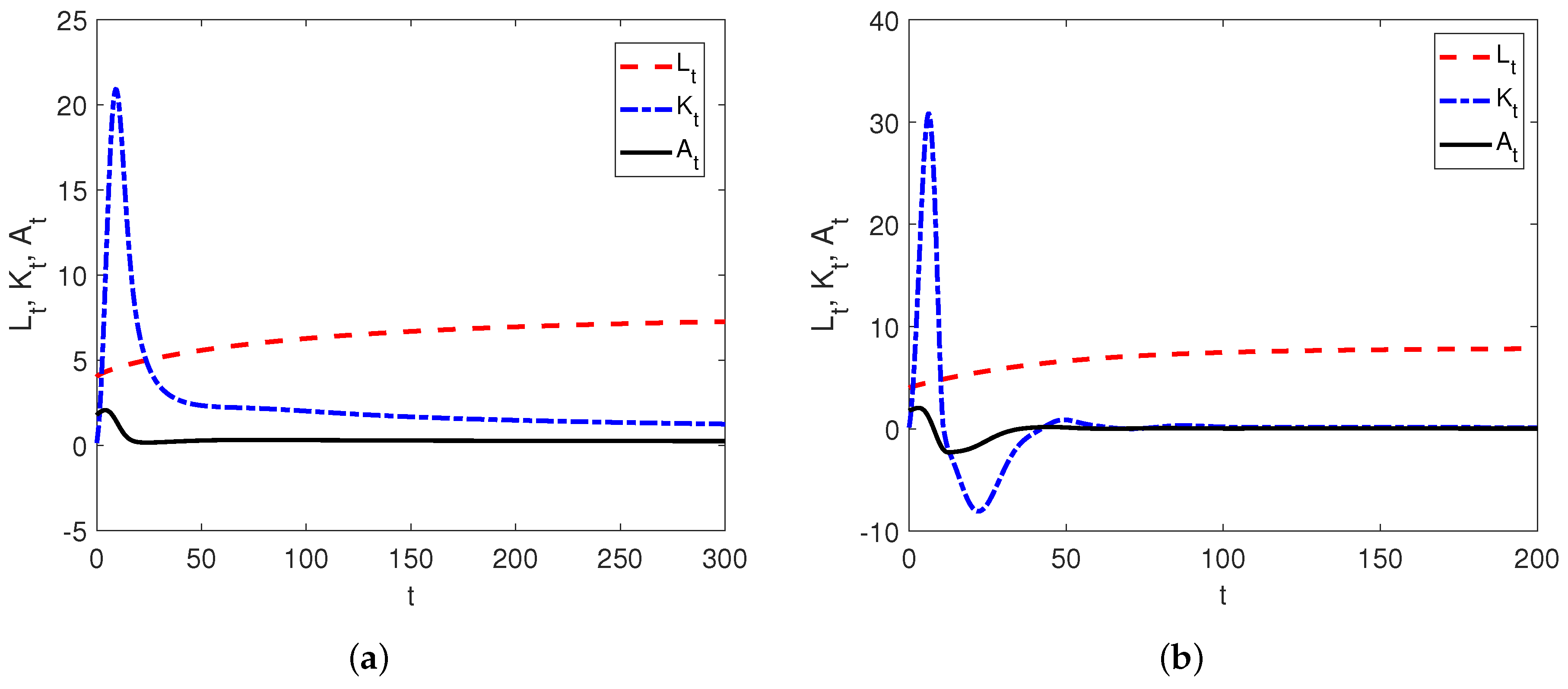
In order to present the dynamic operation state of the fractional order system, some numerical simulations are adopted in this section. Firstly, some numerical examples are given to illustrate the theoretical results above and demonstrate the comparison between the fractional model ($0<q<1$) and the memoryless model ($q=1$). Secondly, a particular case is used to determine the effect of parameter variation on the operation state and the equilibrium point. In the simulation process, we adopt the Adams–Bashforth–Moulton predictor–corrector scheme [39] and take the step-length $h=0.01$.

We assign specific values to some of the parameters in system (8) and consider the following equation

$$\left\{\begin{array}{c}{D}_t^q{L}_t=0.05(1-L_t/8)L_t,\hfill \\ D_t^q{K}_t=0.4A_t{K}_t^{\alpha }{L}_t^{1-\alpha }-0.2K(t-2),\hfill \\ D_t^q{A}_t=p{A}_t+w{L}_t+hK(t-2).\hfill \end{array}\right.$$

(35)

Take the data of China in 1978 as the initial value $E_0=(4.0152,0.1383,1.7788)$.

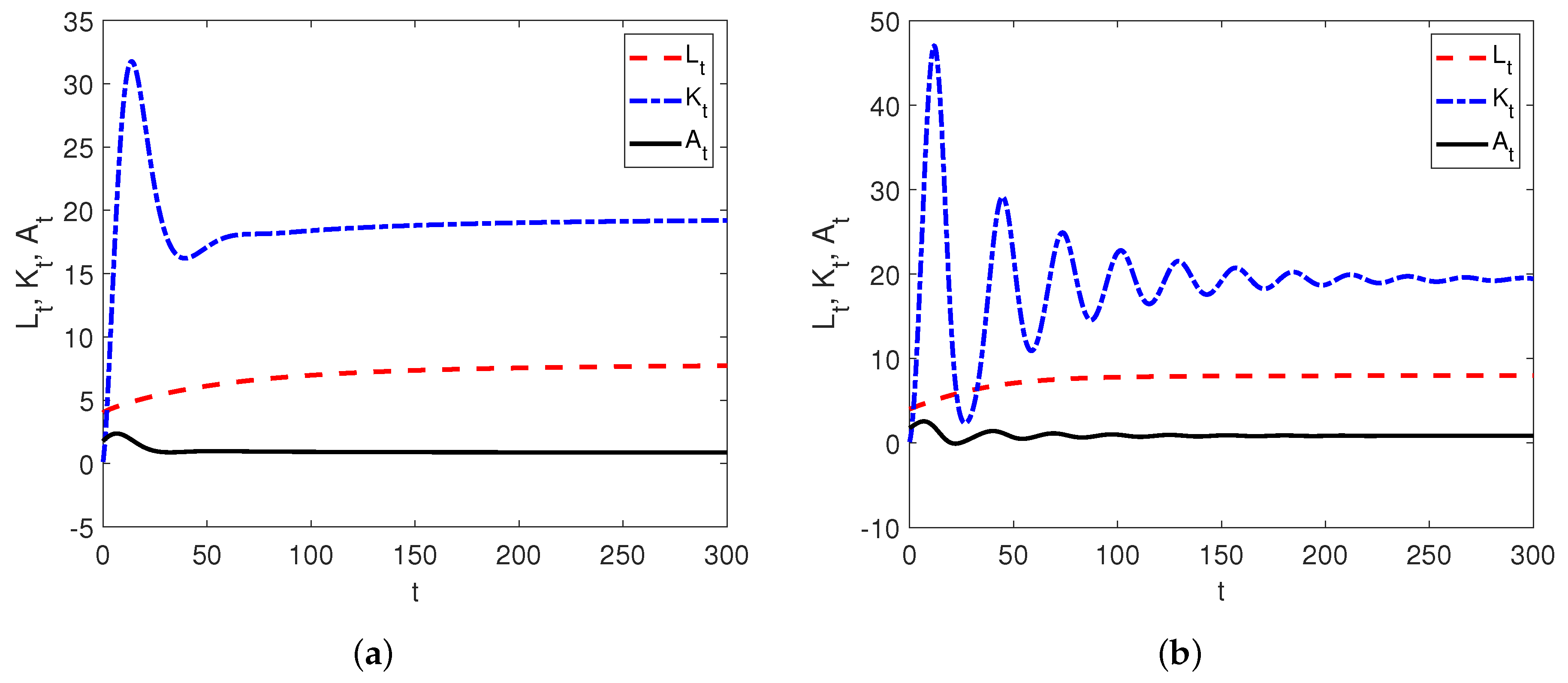
Case 1.

To verify Theorem 1, we set

$$q=0.7,\alpha =0.6,p=0.06,w=0,h=-0.03.$$

The positive equilibrium point of system (35) is calculated to be $\overline{E}=(8.000,0.250,0.125)$. It can be verified that corresponding conditions in Theorem 1 are satisfied. According to Theorem 1, the equilibrium point $\overline{E}$ is Lyapunov asymptotically stable, and the convergence behavior of the response curve is shown in Figure 1a. For comparison, we also simulate the response curve in the case of $q=1$ in Figure 1b.

Figure 1. The timeevolution of System (35) for $q=0.7$ (a) and $q=1$ (b) in Case 1.

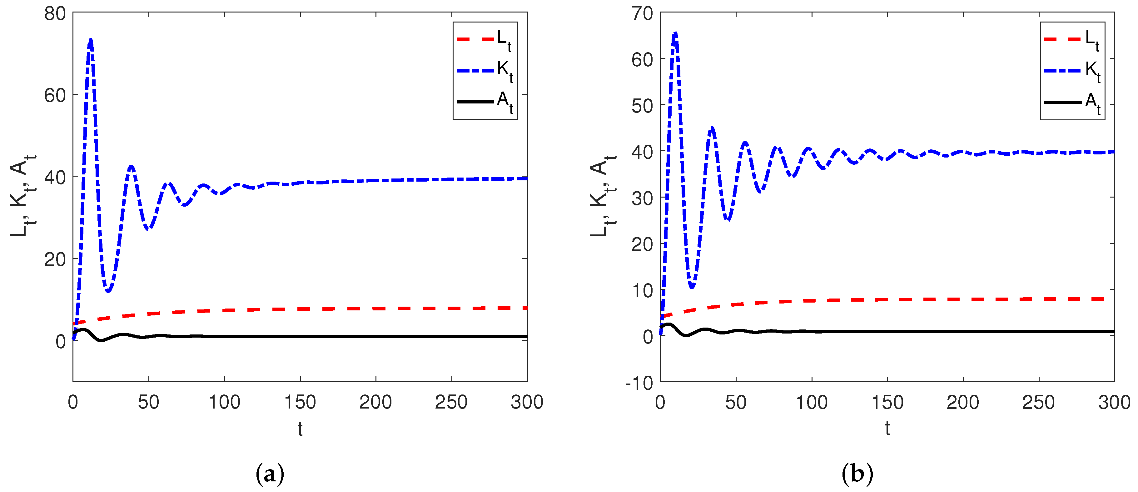
Case 2.

To verify Theorem 2, we set

$$q=0.85,\alpha =0.6,p=0,w=0.05,h=-0.01.$$

The positive equilibrium point of system (35) is calculated to be $\overline{E}=(8.000,40.000,0.952)$. It can be verified that corresponding conditions in Theorem 2 are satisfied, so the equilibrium point $\overline{E}$ is Lyapunov asymptotically stable, and the convergence state of system (35) is shown in Figure 2a. Similarly, when $q=1$, the response curve of the memoryless model is shown in Figure 2b.

Figure 2. The time evolution of System (35) for $q=0.85$ (a) and $q=1$ (b) in Case 2.

Case 3.

To verify Theorem 3, we set

$$q=0.8,\alpha =0.4,p=0.04,w=0.02,h=-0.01.$$

One of the positive equilibrium points calculated by numerical methods is $\overline{E}=(8.000,19.403,0.851)$. It can be verified that corresponding conditions in Theorem 3 are satisfied, so the equilibrium point $\overline{E}$ is Lyapunov asymptotically stable, and the convergence state of system (35) is shown in Figure 3a. For $q=1$, the reponse curve is shown in Figure 3b.

Figure 3. The time evolution of System (35) for $q=0.8$ (a) and $q=1$ (b) in Case 3.

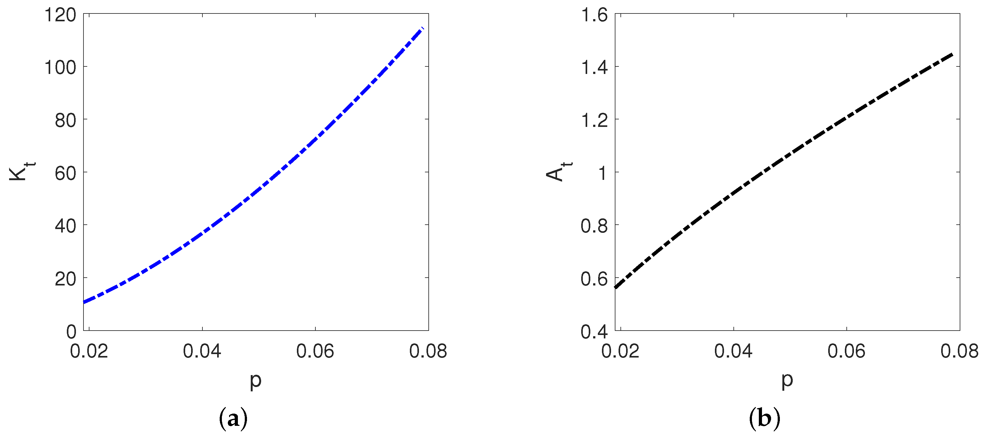
In order to analyze the influence of parameter variation on the equilibrium point and steady state, we perform parameter sensitivity analysis. Take Theorem 1 as an example. The following parameter values are chosen, and we only observe the influence of parameter p on the system.

$$q_1=q_2=q_3=q=0.8,\tau =2,r=0.05,L_m=8,$$

$$s=0.4,\alpha =0.6,\delta +n+g=0.2,w=0,h=-0.001.$$

To obtain a stable equilibrium point, the suitable range of p can be calculated through the stability condition displayed in Theorem 1, that is $p\in (0.019,0.079)$. As p changes within the interval, the equilibrium point keeps Lyapunov asymptotically stable, but the values of the equilibrium point gradually changes, as depicted in Figure 4.

Figure 4. The influence of p on the equilibrium value $K_t$ (a) and $A_t$ (b).

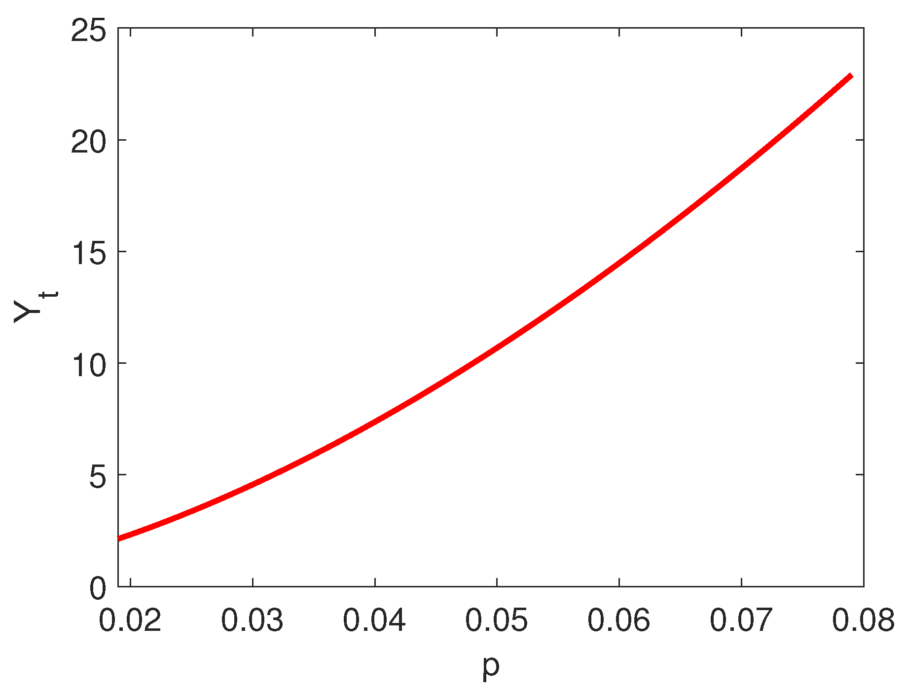
Furthermore, we use the Douglas production function $Y_t=A_t{K}_t^{\alpha }{L}_t^{1-\alpha }$ to calculate GDP value at the equilibrium point, which is shown in Figure 5.

Figure 5. The influence of p on the equilibrium value $Y_t$.

It can be seen that as p increases, the equilibrium value of $K_t$ and $A_t$ are also gradually increasing, which drives GDP to a higher level, indicating economic growth. In system (8), p is TFP growth rate, reflecting the level of technological progress. On the one hand, when p increases, the growth rate of TFP speeds up and stabilizes at a higher level. On the other hand, the acceleration of technological progress promotes capital accumulation, which further has a positive feedback effect on TFP due to endogenous growth. Therefore, under the dual influence of capital accumulation and TFP, the steady-state GDP will rise with the increase in p. The analysis result of the parameter p implies that increasing the TFP growth rate contributes to economic growth. It is consistent with the view that falls in TFP growth appear to explain past growth slowdowns of some middle-income countries [40].

5. Economic Prediction

In this section, we predict China’s GDP in the next thirty years based on model (8) and analyze its economic growth potential. To enhance the adaptability of the model, we allow the fractional orders $q_1,q_2,q_3$ to change dynamically with time t, denoted as $q_1\left(t\right),q_2\left(t\right),q_3\left(t\right)$. For each period t, we use the prediction error minimization principle and the grid search method to find the optimal fractional orders $q_1^{*}\left(t\right),q_2^{*}\left(t\right),q_3^{*}\left(t\right)$. Then, we use curve fitting to predict the trend of $q_1\left(t\right),q_2\left(t\right),q_3\left(t\right)$, and then predict the main variables ($L_t,K_t,A_t$) and GDP($Y_t$) in the next thirty years 2020–2050. Particularly, to clarify the impacts of different fractional derivatives and delay parameters on the predictions, we carefully choose a set of alternative q and $\tau$ to compare their prediction performance.

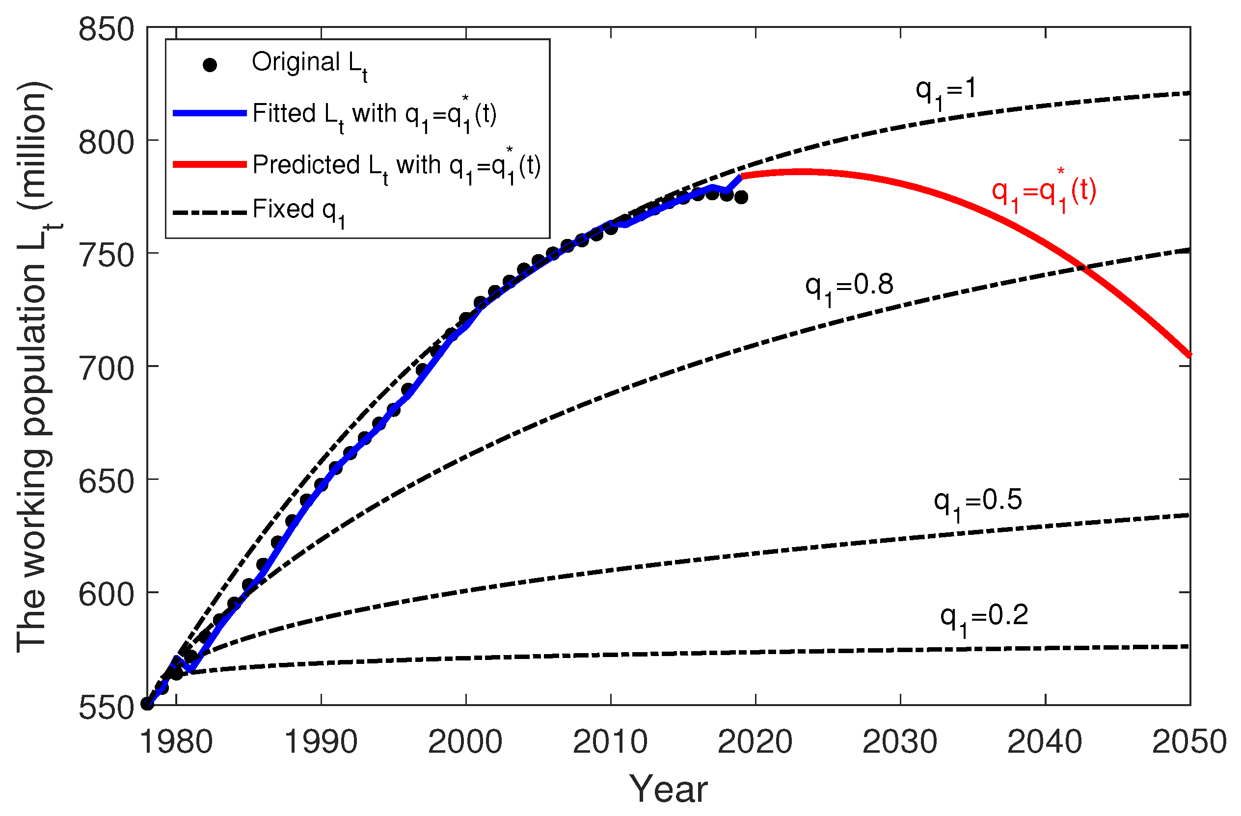
The data is taken from the “China Statistical Yearbook 2020”. It directly provides the working population ($L_t$), total capital formation ($K_t$), and GDP ($Y_t$) from 1978 to 2020. Among them, the working population data appears an obvious gap around 1990 due to the different statistical method used. Therefore, we use the total population to regress and calibrate the working population by Ordinary Least Squares (OLS). For TFP, we use the Cobb Douglas function $Y=A{K}^{\alpha }{L}^{1-\alpha }$ to calculate A as the true value of TFP, where the contribution ratio of capital to output $\alpha$ is 0.6 as general.

Next, we set the parameters in system (8) For working population $L_t$, we fit the integer-order population retardation growth model and get the growth rate $r=5.55\%$ and the maximum population $L_m=828.38$ million. Secondly, according to the final consumption rate data in 1978–2020, we set the average savings rate $s=41.22\%$. In addition, consulting relevant information, we take the contribution ratio of capital to output $\alpha =0.6$, the depreciation rate $\delta =5\%$, the technological progress rate $g=2\%$, and the natural population growth rate $n=5\%$. For the sake of simplicity, we set $w=h=0$, that is, the third equation in system (8) is simplified to $D_t^{q_3\left(t\right)}{A}_t=p{A}_t$.

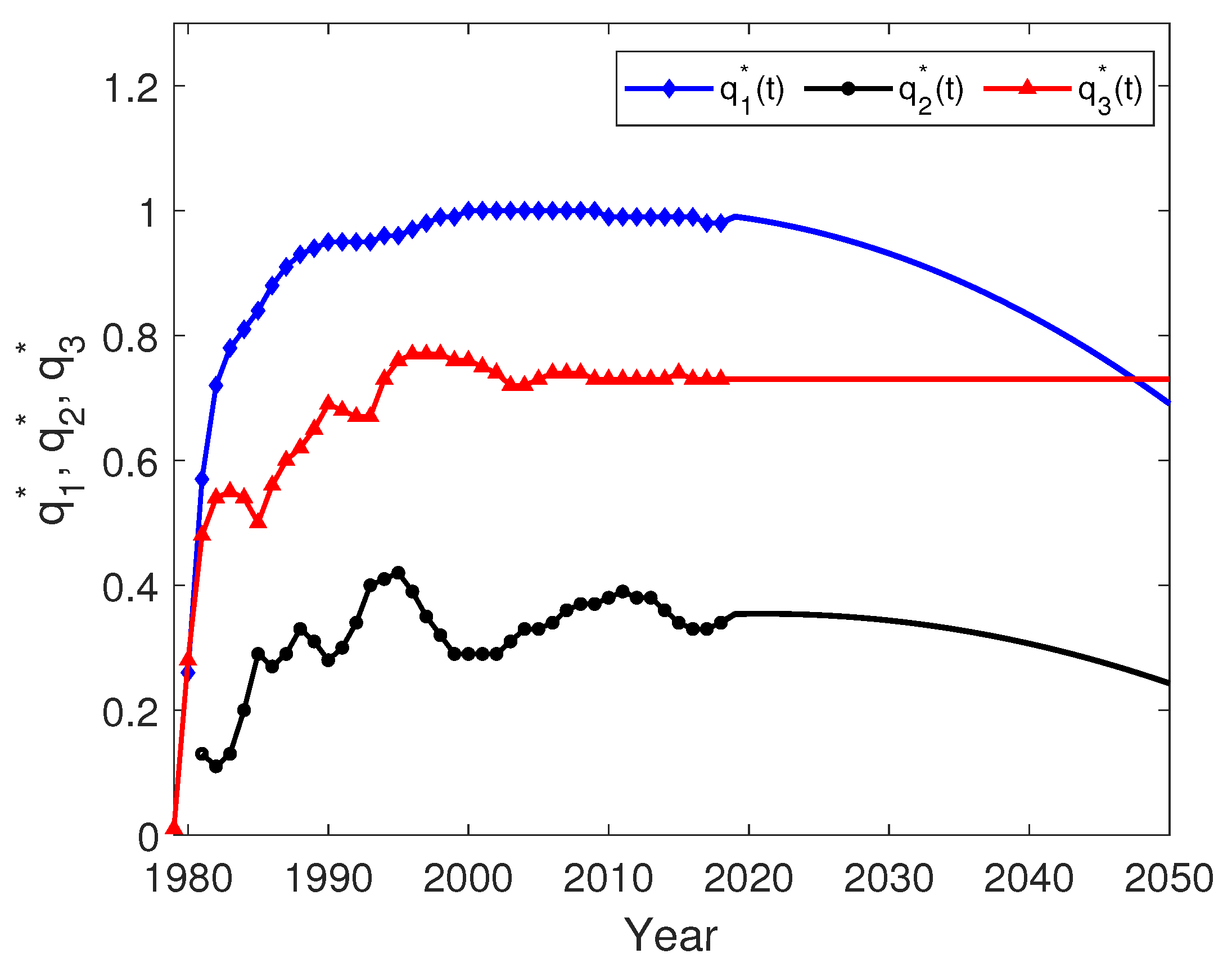
After the necessary data is ready, we start to make predictions. Above all, we show our approach to choose the suitable fractional derivative parameters $q_1$, $q_2$, $q_3$. To make the prediction more time-varying, we dynamically change the fractional derivative orders with time so that they turn into functions of t, i.e., $q_1\left(t\right),q_2\left(t\right),q_3\left(t\right)$. We now use the existing data and model to solve them. Taking $q_1\left(t\right)$ as an example, we optimize it by minimizing the prediction error and obtain

$$q_1^{*}\left(t\right)=argmin\parallel L_t-\widehat{L_t}\left(q_1\left(t\right)\right)\parallel ,q_1^{*}\left(t\right)\in (0,1),$$

(36)

$$D_t^{q_1\left(t\right)}{\widehat{L}}_t=r(1-{\widehat{L}}_t/L_m){\widehat{L}}_t,$$

where $\parallel ·\parallel$ is 2_norm. To solve (36), for each period t ($1980⩽t⩽2020$), we perform a grid search on $q_1\left(t\right)$ within the interval (0,1) by step length of $h=0.01$. In particular, ${\widehat{L}}_t\left(q_1\left(t\right)\right)$ is figured out by the predictor–corrector method. For $t>2020$, we fit $q_1\left(t\right)$ with a quadratic function and forecast its trend in the next thirty years as shown in Figure 6 (the blue line). Using the same method, we can obtain the optimal $q_2^{*}\left(t\right)$ and $q_3^{*}\left(t\right)(1980⩽t⩽2020)$ by minimizing the prediction error. As shown in Figure 6, $q_3^{*}\left(t\right)$ (the red line) finally stabilizes at 0.73 around 2020, so we directly let $q_3\left(t\right)\equiv 0.73$ when $2020<t⩽2050$. As for $q_2$ (the black line), we also perform a quadratic function fitting on $q_2^{*}\left(t\right)$ and predict its value in 2020–2050.

Figure 6. Optimal $q_1^{*}\left(t\right),q_2^{*}\left(t\right),q_3^{*}\left(t\right)$ and their predicted value in 2020–2050.

Based on $q_1^{*}\left(t\right)$, we can calculate ${\widehat{L}}_t$ according to Equation $D_t^{q_1^{*}\left(t\right)}{\widehat{L}}_t=r(1-{\widehat{L}}_t/L_m){\widehat{L}}_t$ using the predictor–corrector method. The fitted $L_t(1980⩽t⩽2020)$ and the predicted $L_t(2020<t⩽2050)$ are shown in Figure 7.

Figure 7. The impacts of different fractional derivatives $q_1$ on the prediction of $L_t$.

The memory parameter q plays a significant role in our framework. However, it is currently practically not studied in econometrics. Therefore, it is interesting and meaningful to explore its role in economic operations and its impact on economic predictions. We consider a wide range of $0<q<1$$(q=0.2,0.5,0.8)$ as well as the memoryless model $q=1$. Then, we take $q_1$ as these fixed values and predict $L_t$ in 1980–2050. As shown in Figure 7, when $q_1$ decreases, the predicted working population $L_t$ declines, indicating that $q_1$ describes the growth rate of population. In addition, compared with the optimal $q_1^{*}\left(t\right)$, the memoryless $q=1$ overestimates the working population, especially when $2020<t⩽2050$, while $q=0.8,0.5,0.2$ greatly underestimates the working population.

The consideration of fractional derivatives does capture the memory and heredity feature in the population growth process, with its prediction more accurate. However, the fractional order parameters need to be carefully selected. Our method of minimizing the prediction error is proven to be an effective and precise approach to select the fractional derivative orders.

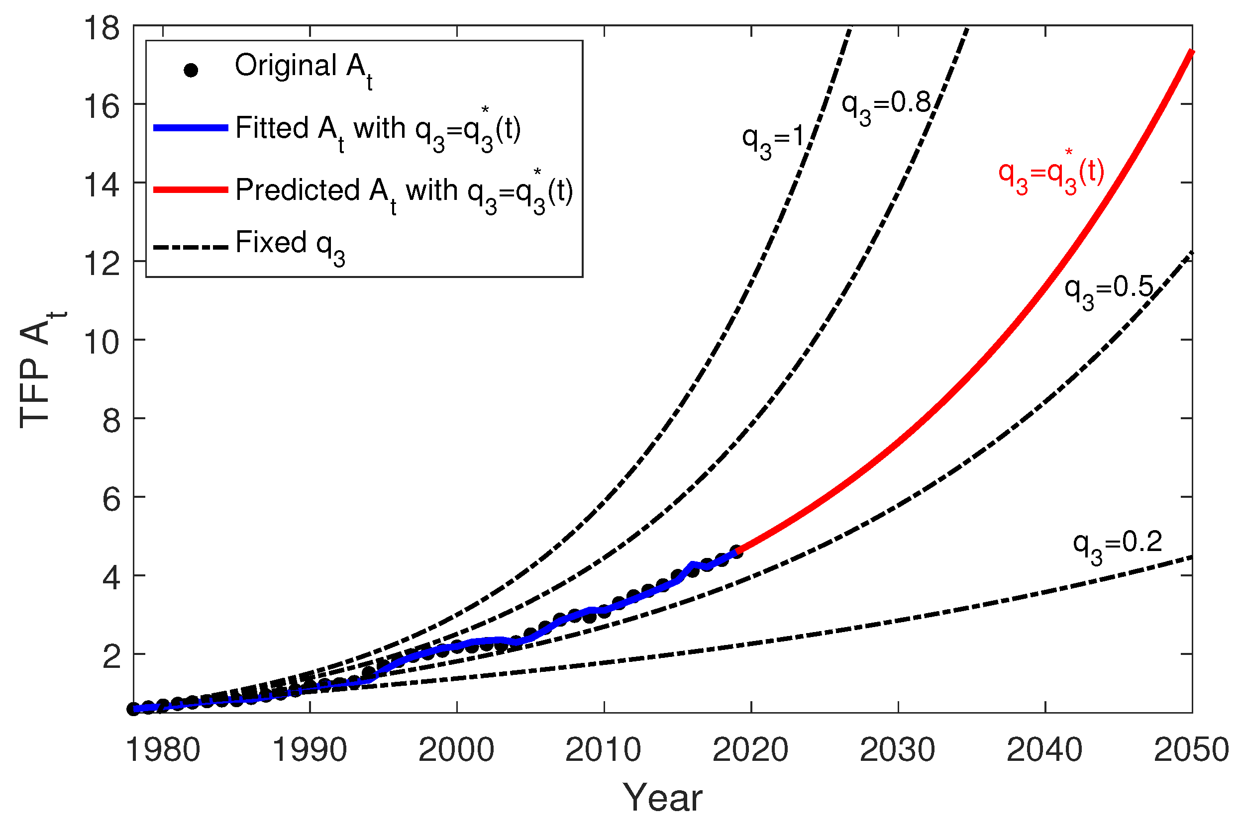
Similarly, based on the calculated $q_3^{*}\left(t\right)$ and the equation $D_t^{q_3^{*}\left(t\right)}{\widehat{A}}_t=g{\widehat{A}}_t$, we can obtain the fitted and predicted ${\widehat{A}}_t$, as shown in Figure 8. We also compare the prediction performance of $q_3=q_3^{*}\left(t\right)$ with a wide range of $0<q_3<1$ and $q_3=1$. As reflected in Figure 8, we conclude that the growth rate of TFP rises with the increase in $q_3$ and $q_3=q_3^{*}\left(t\right)$ outperforms other fixed $q_3$.

Figure 8. The impacts of different fractional derivatives $q_3$ on the prediction of $A_t$.

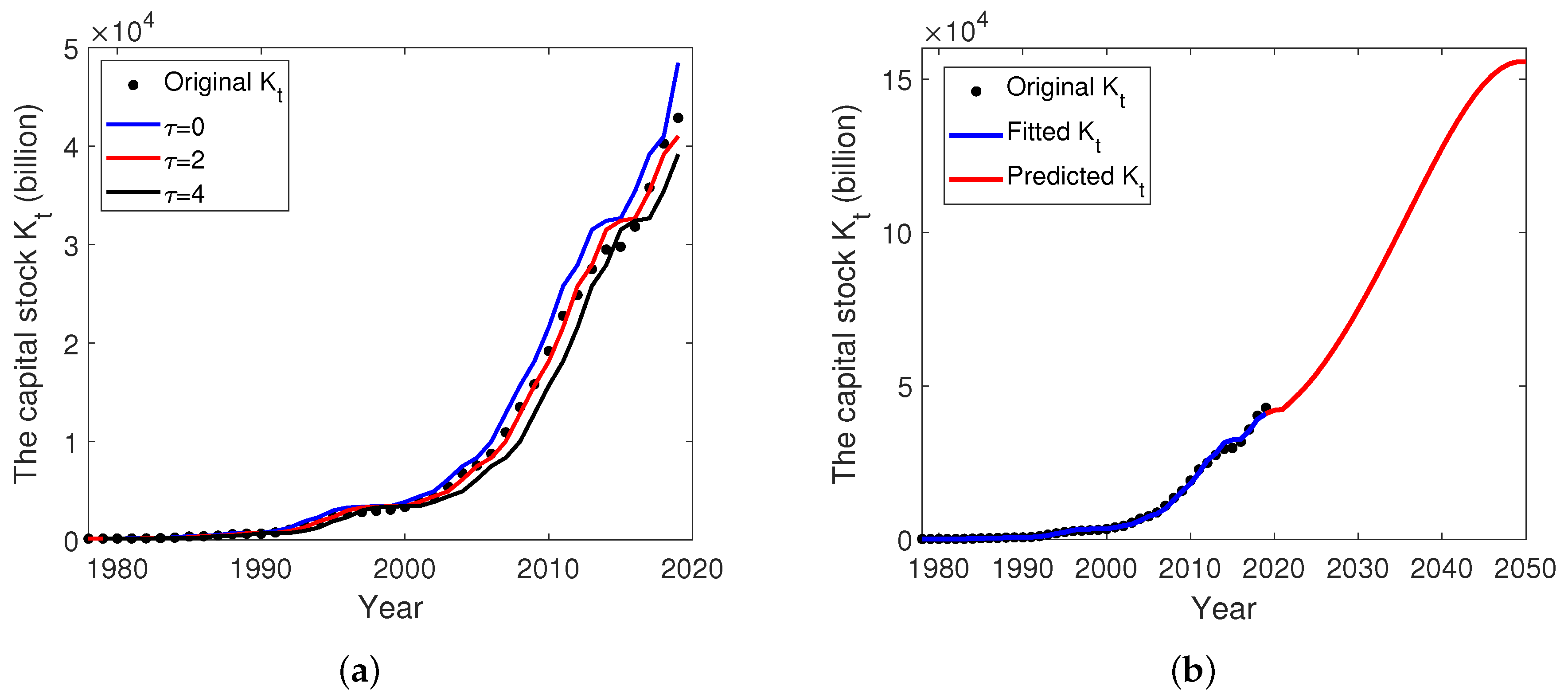
As for the capital stock $K_t$, we have the equation $D_t^{q_2\left(t\right)}{K}_t=s{A}_t{K}_t^{\alpha }{L}_t^{1-\alpha }-(\delta +g+n)K(t-\tau )$, where $A_t$ and $L_t$ are replaced by the predicted values $\widehat{A_t}$ and $\widehat{L_t}$, respectively. To select the suitable delay parameter $\tau$ as well as examine the impacts of time lag on the predictions, we evaluate the prediction performance in three cases, namely no delay case $\tau =0$, medium delay case $\tau =2$ and high delay case $\tau =4$. Similarly, the predictor-corrector scheme is used again to solve ${\widehat{K}}_t$. The fitting results of different delays are depicted in Figure 9a.

Figure 9. The impacts of delay $\tau$ on the fitted $K_t$ (a). The predicted $K_t$ in 2020-2050 with $\tau =2$ (b).

As can be seen in Figure 9a, the fitting result of the medium delay case $\tau =2$ best matches with original $K_t$, so we choose it for our thirty-year prediction. It is worth noticing that $\tau =0$ represents the no delay case, which slightly overestimates the capital stock. It is because $\tau =0$ means that $\Delta K_t$ is merely determined by $L_t,K_t,A_t$ at time t, while ignoring the historical state. In contrast, the time lag can take into consideration the previous values of economic variables in the capital accumulation process and emphasize the impact of historical data on the current $\Delta K_t$. It offsets the overestimation compared with the no delay case and largely improves the prediction performance. Therefore, we use $\tau =2$ and $q_2^{*}\left(t\right)$ to predict ${\widehat{K}}_t$ when $2020<t⩽2050$ as shown in Figure 9b.

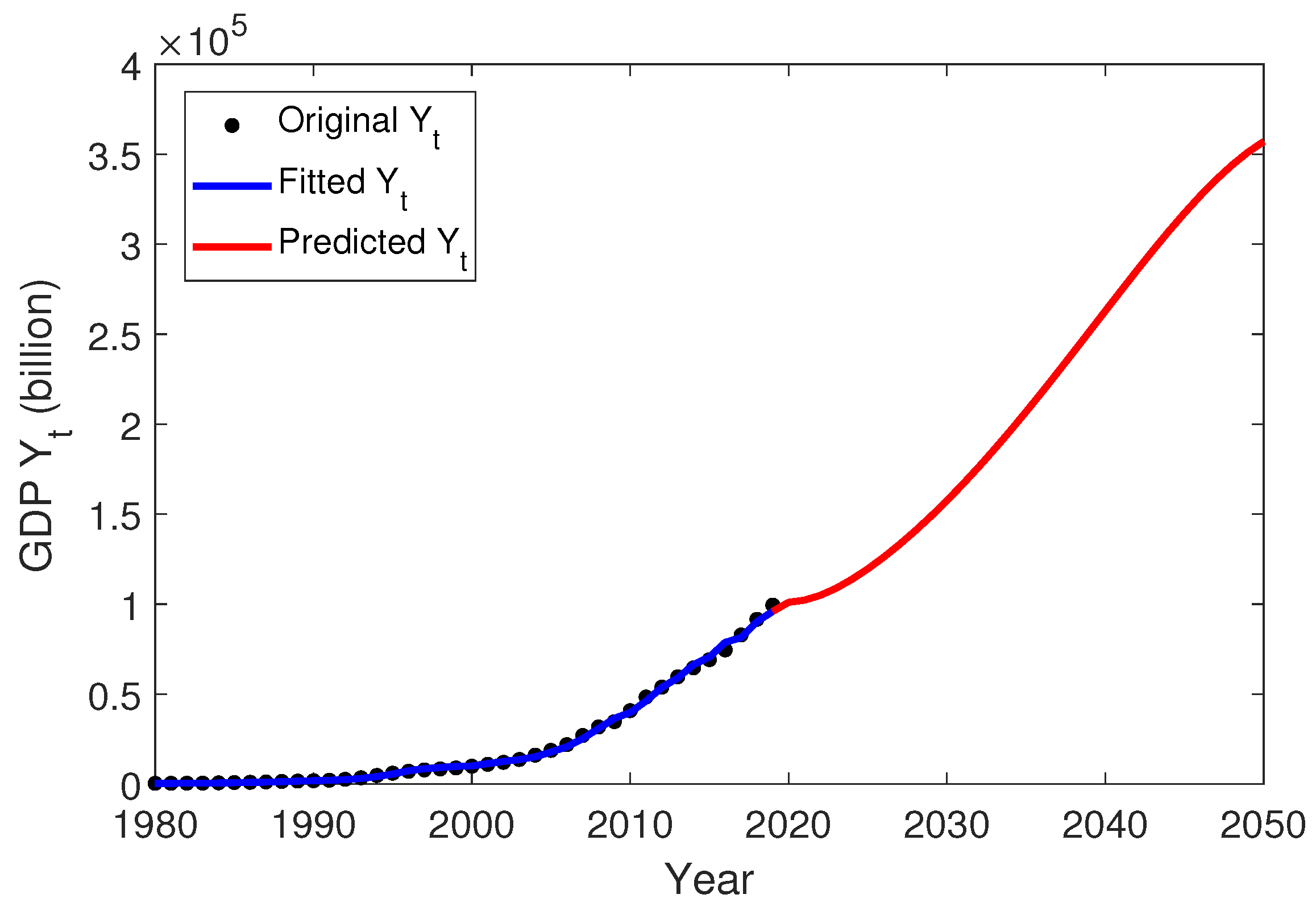
Finally, by using $Y=A{K}^{\alpha }{L}^{1-\alpha }$ and the predicted values of $\widehat{L_t}$, $\widehat{A_t}$, and $\widehat{K_t}$, we can easily get the predicted GDP ($\widehat{Y_t}$) for each year, as shown in Figure 10.

Figure 10. Fitted GDP and predicted GDP of China in 2020–2050.

We now describe and analyze the prediction results from economic perspective. In Figure 6, the fractional order $q_1\left(t\right)$ peaked around 2010 and then began to decline, leading to a downward trend in the working population ($L_t$) since 2020, as shown in Figure 7. The decrease in the working population was attributed mainly to the government-sponsored family planning program and the so-called “one-child policy” introduced in the 1970s. The policy led to a sharp decline in total fertility rate and the acceleration of population aging [41]. Consequently, the shrinking of the working population occurred and will probably continue in the approaching half a century [42].

As for the prediction of TFP, since the fractional order $q_3\left(t\right)$ reached a plateau after 2000, fluctuating slightly around 0.73, TFP in 2020–2050 will probably continue to increase following the previous trend. In a developing country like China, the increase in TFP is largely caused by the “catch-up effect” which comes from the process of catching up from post-developed countries to developed countries. Evidence from multiple nations shows that if developing countries make full use of the advantages of chasers, they have the opportunity to accelerate development [43].

Figure 9b indicates that the capital stock still holds an upward trend, but the growth rate will slightly slow down. The increase in capital stock makes it possible for developing countries to take advantage of advanced technology and accelerate productivity, which has a significant positive long-term impact on economic growth [44]. Furthermore, the positive feedback is expected to continue in the short term according to the prediction.

Finally, as can be seen in Figure 10, China’s GDP will continue to grow at a medium-to-high speed in the next five years, approaching about $3.5\times {10}^5$ billion in 2050. Despite a slight decrease in the working population, the increase in capital stock and the rise in TFP still provide persistent and vigorous impetus to economic growth.

However, in this paper, it is worth emphasizing that China will encounter multiple obstacles on the road to economic growth, and these impediments have already emerged in our forecasts. On the one hand, the decline in the working population is an inevitable trend, which indicates the disappearance of the demographic dividend. On the other hand, although the capital stock is still growing, the growth rate has shown signs of decelerating. We should have a clear understanding that the high-speed economic growth path derived by the accumulation of capital is unsustainable and will eventually come to an end in the long run. When capital is accumulated to a certain level, China will probably experience the development predicament like other developed countries such as Japan and South Korea. Therefore, in order to break through the dilemma, we should focus on TFP. According to the regularity of economic growth mode, the high contribution of TFP to economic growth usually appears when entering the mature period of growth deceleration [45]. In other words, China needs to transform its economic growth into a trajectory dependent on TFP growth. In our forecasting model shown as Figure 8, TFP is still growing along the trend in the short term, which, therefore, leads to sustainable economic growth. In conclusion, increasing the contribution rate of TFP in the future is the core goal and new engine of China’s economic growth.

6. Conclusions

In this paper, a delayed fractional differential equation model was established. The time delay introduced into the capital stock is to characterize the lag effect and memory features in economic operations. We used the stability theory of fractional-order system with time delay and obtained the sufficiency condition for the local stability of the equilibrium point. In the numerical simulation, we selected appropriate parameters according to the corresponding conditions and drew the response curve. We also compare the memoryless model of $q=1$ with the factional one and verify the correctness of the theoretical results. Furthermore, to analyze the influence of parameter variation on the equilibrium point and steady state, we performed sensitivity analysis on the typical parameter p, and found that the increase in TFP growth rate contributes to economic growth.

In the application section, we predicted China’s GDP growth in the next thirty years based on the fractional derivative economic growth framework. In the prediction, the fractional derivatives and delay parameters are carefully selected by the minimum prediction error principle. We also explore the impacts of fractional derivatives and delay on predictions and clarify the economic implications and stylistic facts brought by the two additional features. Forecast results suggested that China’s economy would continue to grow at a medium-to-high speed. In addition, we successively forecasted the working population, capital stock, and TFP as by-products. A downward trend in the employment population and a potential slowdown in capital stock growth emerge, which forces us to focus on TFP. TFP measures the efficiency of resource development and utilization, which is directly and highly related to the level of technology. Therefore, only by achieving technological progress and increasing TFP can the pressure on the working population and capital stock be offset, and economic growth can be sustained.

Economic growth is a goal pursued persistently by countries all over the world. We will collect more economic data from other countries in the future and use the proposed model to analyze the economic growth. We will improve the model according to the characteristics of different countries, hoping to obtain a more general and widely applicable theoretical framework.