


The Prediction of the Compaction Curves and Energy of Bituminous Mixtures

Abstract
1. Introduction
- On-site variables. Some variables, such as asphalt mixture properties, can be controlled during the design phase. Others, such as aspects of the construction process, are managed by contractors during the construction phase. The factors include the following: (1) The type and density of the underlying base course material (when on-site compaction is concerned). To this end, it is noted that the compaction energy depends on the type of underlayer material (e.g., subgrade soil, aggregate base course, cold mix asphalt layer, cracked friction course, new asphalt concrete layer, or a Portland cement concrete pavement layer). (2) The thickness of the asphalt layers. Indeed, thinner asphalt layers could cool faster than thicker layers. It is noted that for finer-density graded mixes (above the 0.45-power chart maximum density line), the minimum lift thickness should be three times the nominal maximum aggregate size. However, for a coarse-graded mix (below the maximum density line), the lift thickness should be at least four times the nominal maximum aggregate size. (3) The environmental conditions at the time of placement (see below). (4) The on-site procedures and machines, including the type of rollers, the number of rollers, and the rolling patterns used during the compaction process. (5) The mix temperature.
- Environmental conditions. Environmental conditions (e.g., ambient temperature, wind speed) also play a crucial role [7]. For the environmental conditions at the time of mix placement, note that air temperature, base temperature, wind velocity, and solar flux or cloud cover influence the compaction and the cooling rate of the mix.
- Bitumen. Asphalt binder percentage (lubricating effect) and type, where different methods of classifications are given (penetration-based, viscosity-graded, AC, and performance-graded, PG) and different strategies are followed, including polymer-modified binders (using either elastomeric- or plastomeric-type materials) and crumb rubber + binder blends (including asphalt rubber).
- Aggregate. Aggregate grading plays a pivotal role in determining the compaction behaviour of asphalt mixtures [8,9]. In more detail, aggregate type, grading, and characteristics, including angularity (cf., fine aggregate angularity, FAA, and coarse aggregate angularity, CAA) are important. There are many aggregate types, including sedimentary rocks (e.g., limestone), igneous rocks (e.g., basalt and granite), and their properties (e.g., absorption, soundness, angularity, surface texture, degree of flat and/or elongated particles, and percentage of crushed rocks) affect the compactability of the resulting mixture.
- Filler. The filler percentage and type affect compaction. Furthermore, the dust proportion (the filler to bitumen ratio) may also affect compaction.
- Type of mixture. The type of bituminous mixture, e.g., dense-graded mixes, DG, (fine-graded, coarse-graded, densely-graded mixes), gap-graded mixes, open-graded mixes, OG, (as a friction course or as a base layer), and stone matrix asphalt, SMA, mixes, influences the final result. Importantly, several factors may cause mixtures to be stiff or tender, including the following: (1) An excessive moisture content. (2) Excessive light ends in the asphalt cement. (3) An excess bitumen percentage. (4) Rounded aggregate particles (cf., FAA and CAA parameters). (5) An excess percentage of fine aggregate (0.3–0.6 mm). (6) An insufficient filler percentage (<0.075 mm). (7) Poor bonding to the underlayer pavement. (8) An excessive mix temperature. (9) Poor compaction techniques (quick stops and starts by a steel-wheeled roller, need for pneumatic tyre rollers). (10) Contamination with petroleum products.
1.1. Compaction Energy in the Laboratory and On-Site: An Analysis of the Literature
- Nini.
- Ndes.
- Compaction energy index (CEI).
- Locking Point (LP).
- Compaction densification index (CDI).
- Traffic densification index (TDI).
- Nmax.
- On-site versus in-laboratory compaction
1.2. Objectives of the Study
2. Materials and Methods
2.1. Modelling
- Reaching Ndes (i.e., the corresponding AV content, e.g., 4% for a dense mixture) is the main aim of the compaction effort. This implies that the LP should be higher than Ndes. On the contrary, the constraint at Nmax does not conflict with having the LP between Ndes and Nmax, nor with having the LP higher than Nmax.
- Having the LP in between Ndes and Nmax could allow reaching the required requirements through lower energy.
- The fact that the LP must be higher than Ndes implies that the function min abs (LP-Ndes) could not fulfil the rationale behind the compaction effort.
- On the other hand, having, as an objective, the function min (LP-Ndes) could be fallacious because of the need to have LP > Ndes.
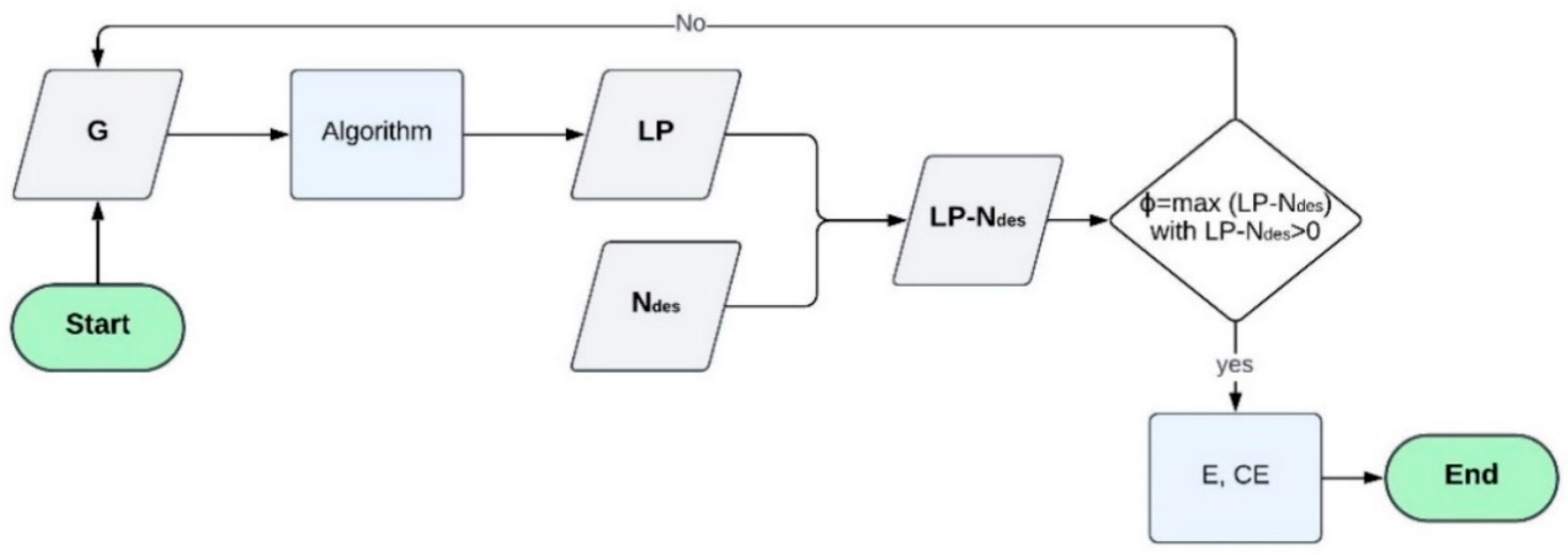
- Based on the above, the objective function max (LP-Ndes), with LP-Ndes > 0 as a threshold value, is here tentatively set up (Equation (1)).
- The in-lab compaction energy can be estimated by using key compaction parameters derived from the compaction curve, such as the CDI and the LP.
- The CDI is proportional to the compaction effort applied in the laboratory (and thus to the energy needed to achieve a given density). It is a useful measure for predicting on-site compaction efforts from laboratory data.
- The LP is a key indicator in this derivation as it translates into the optimisation of aggregate packing without the risk, for example, of over-compaction, which could lead to aggregate damage.
- By integrating the CDI and LP into the analysis, the in-lab compaction energy can be used to predict the energy required for on-site compaction. This prediction accounts for factors such as the mixture composition and design requirements, allowing for the optimisation of both the mixture and the pavement design.
- The on-site compaction energy density (Joule/kg), which is provided by the rollers during the rolling process, should be consistent with the compaction energy density obtained in the laboratory (see [3]).
- On the one hand, the relationship between the energy density associated with compaction and the CDI is mixture-specific because of the many variables involved in both the production and construction processes; on the other hand, the on-site compaction energy can be derived by considering roller-specific parameters (i.e., type, weight) and the number of passes required to obtain the specific degree of compaction.
- Based on the above, the on-site compaction energy should be scaled from lab-derived values using mixture-specific coefficients and field parameters to ensure that the field compaction process meets the density and structural integrity requirements.
- Under the hypothesis of having different pavement technologies to compare, where the grading and the additives are different but comply with the contract specifications, the method set up herein could have the potential to allow the derivation of a further key performance indicator (KPI) useful for both energy estimation and sustainability assessment. Competitive equilibria among different technologies can be analysed by considering the environmental impact and expected life of each concurrent pavement technology (cf. [4]).
2.2. Derivation of the Parameters of the Model
- The selection of materials and data collection. Twenty-two asphalt mixtures were designed and tested. This dataset was increased using data from the literature to extend the range of the analysis.
- The compaction curve analysis. The Superpave Gyratory Compactor (SGC) was used to compact cylindrical specimens for each mixture. By analysing the resulting compaction curves, the LP was determined for each mixture.
- The correlation Analysis. Pearson correlation coefficients were analysed to assess the relationship between compaction-curve-related parameters and the aggregate grading and between the LP and the aggregate gradation parameters (e.g., passing percentages for different sieve sizes, fine content, and dust content).
- Regression modelling. A multivariable regression analysis was carried out to develop a predictive model for both the compaction curve parameters and the LP, based on aggregate-grading-related variables. The accuracy of the model was evaluated by comparing the predicted values against the observed data.
- The Ndes and LP analyses. For each mixture, the relationship between the LP (predicted values) and the Ndes (the values set up in the contract specifications as a part of the job mix formula) was analysed. The model set up above, where the proximity of the LP to Ndes from the right is an indicator of the energy efficiency of the mixture, was implemented and validated.
- Remaining steps. The remaining steps are as follows: (6.1) The estimation of the in-lab and on-site compaction energy. (6.2) The analysis of competitive equilibria and the derivation of the targets for the optimisation of the mixtures.
- The percentage passing (Pi) through the following sieves (i): 20, 16,12.5, 9.5, 4.75, 2.36, 1.18, 0.6, 0.3, 0.15, 0.075 mm.
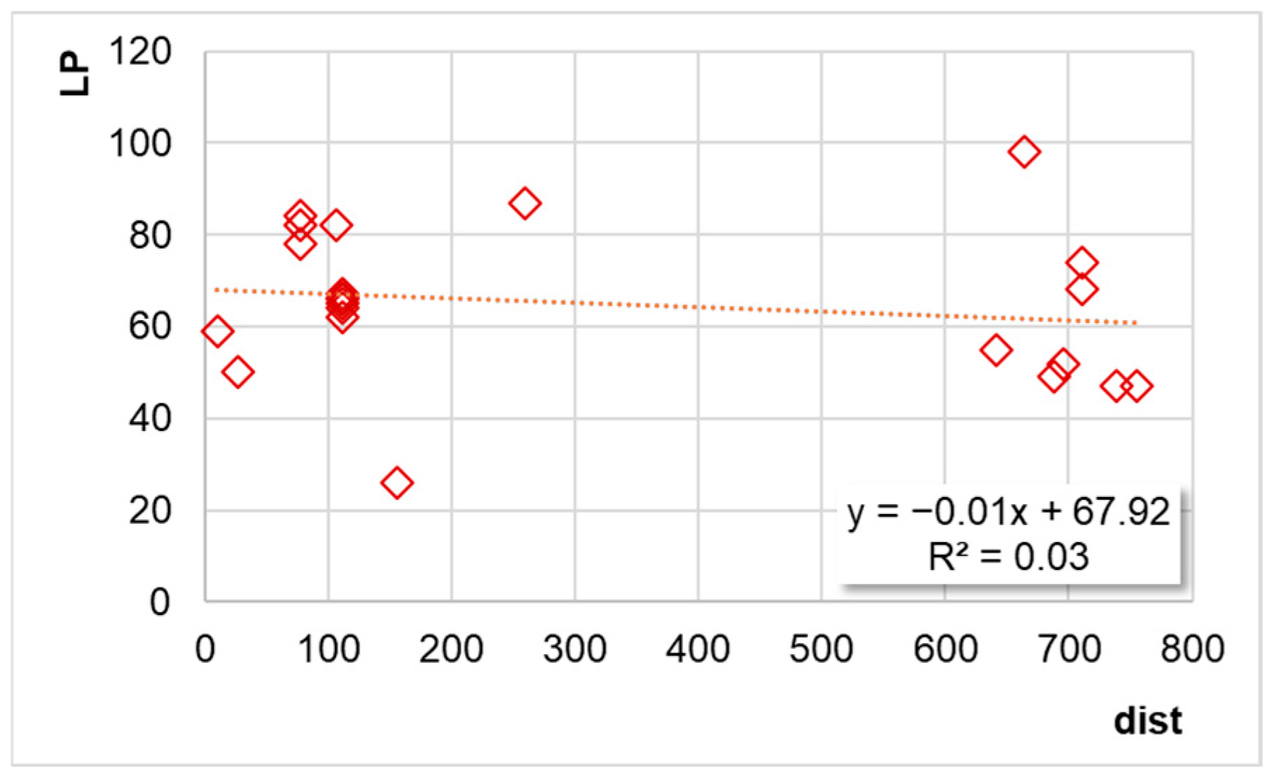
- The squared distance from the maximum density line, dist (Equation (2)), defined as the square of the average distance between the maximum density curve and the actual gradation (considering the following sieves 31.5, 20, 16, 12.5, 8, 4, 2, 0.5, 0.25, and 0.075 mm).where Pi is the percentage passing through the sieve size i, Si is the sieve size i, and Smax is the maximum sieve size where the passing percentage is 100%.
- Sand or fine percentage, sand (the percentage passing through the 2.36 mm sieve and retained on the 0.075 mm sieve).
- Dust (or filler) percentage, dust (the percentage passing through the 0.075 mm sieve).
- Coarse aggregate, coarse (obtained as 100 − P2.36).
2.3. Materials
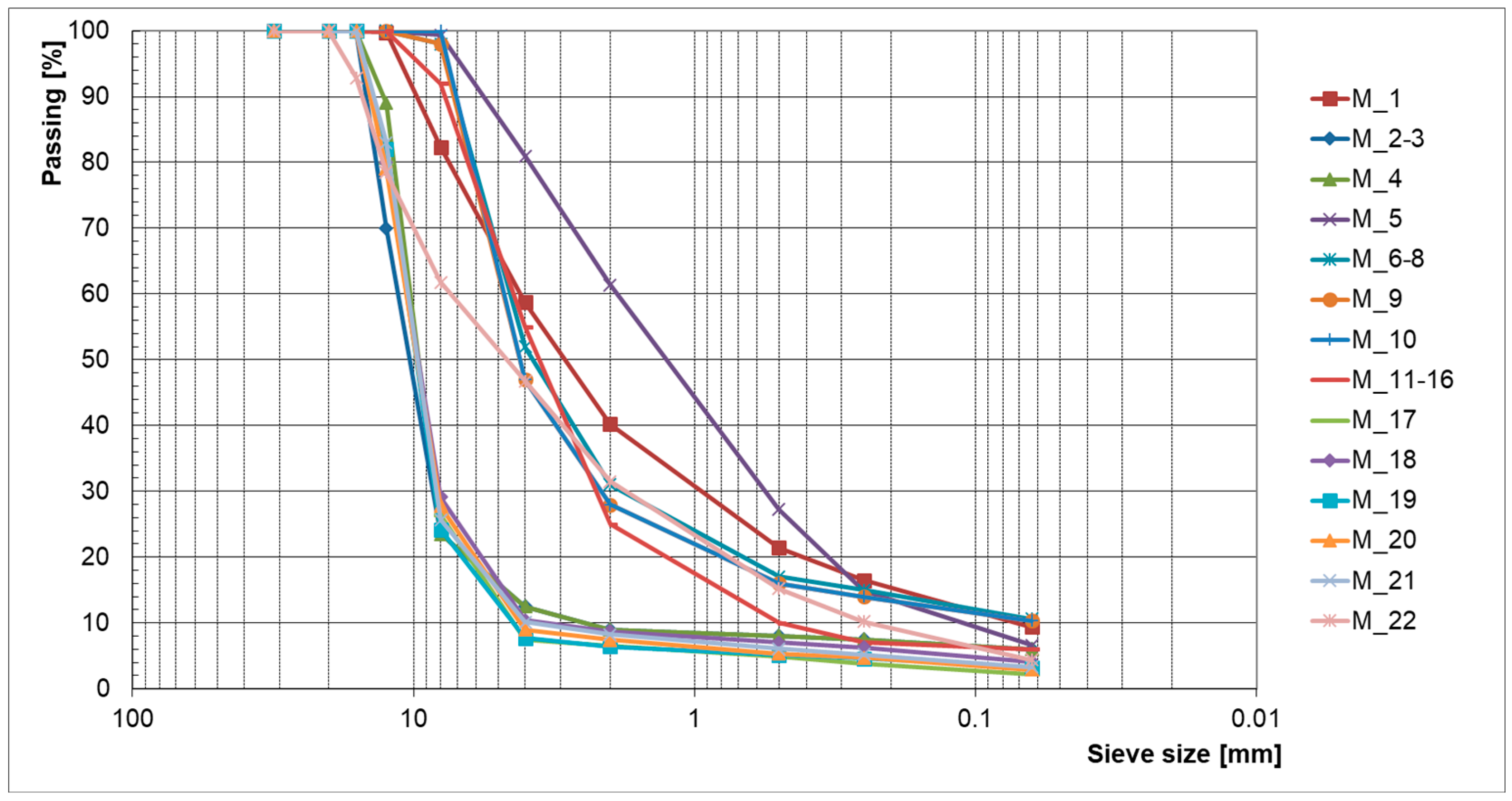
- The gradation of the mixtures produced and tested in this study (Figure 3);
3. Results and Discussion
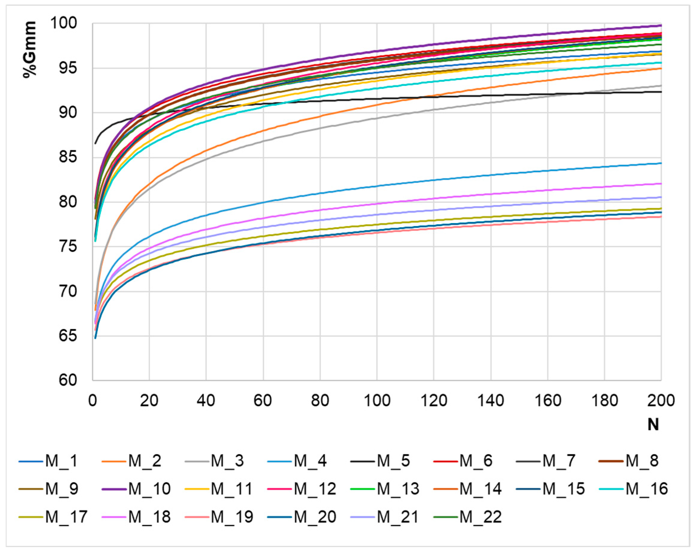
3.1. Compaction Curves
- The power law (Equation (3)):
- The logarithm law (Equation (4)):
- The three-parameter quotient (Equation (5)):
- The Moutier model (Equation (6)):where N is the number of gyrations, and a, b…m, C0, C∞, β3, and β4 are the fitting parameters. Note that
- The first and second models are the ones commonly used.
- The three-parameter quotient is herein set up to properly account for %Gmm variability, where two theoretical requirements should be fulfilled: (1) Having a reasonable upper limit of %Gmm for an N that tends to infinity (i.e., l ≤ 100%). (2) Having a reasonable behaviour close to zero (e.g., h/m ≅ 55–90%).
- The Moutier model [32] has four parameters. It has an upper limit (when N tends to infinity) and a lower limit different from 0 (when N tends to 0). Unfortunately, the exponent is linked to the difference between the upper and lower levels, and this could cause issues when fitting real curves.
- The power law and the logarithm law fail to represent what happens at the beginning of the compaction procedure, where, as a result of gravity (as well as the normal pressure applied), the density has a given finite value, different from zero. Here, it is noted that not only do the two models fail to represent what happens (cf., “–” and “NA” in Table 3), but, at the same time, what happens in the laboratory could be quite different from what happens on-site. Indeed, the initial pressure (600 kPa) exerted by the head of the gyratory compactor does not seem to represent the action of gravity + paver bar well. Further studies will be needed. From a practical standpoint, this issue at N = 0 could have more theoretical than practical consequences, simply considering what happens at N = 1 or N = 8.
- The power law and the logarithm law fail to represent what happens for a high number of gyrations. Indeed, when N increases for sample heights, it should be hmin ≤ h(N) and for air voids, AV = 1 − Gmb/Gmm ≥ 0. Consequently, for %Gmm, it should be %Gmm = Gmb/Gmm = hmin/h(N) ≤ 100%. For the sake of comprehensiveness, slight deviations from the equations above could happen because of a change in Gsb due to aggregate pulverisation, but these inconsistencies of the two models above remain clear.
- For the Moutier model mentioned above, in contrast with the aim (i.e., having a reasonable upper limit when N tends to infinity), for actual curves, the boundary condition for %Gmm (i.e., C∞ ≤ 100%) is usually not fulfilled (cf., Table 3). Importantly, values higher than 100% for C∞ were also obtained by [33]. The theoretical problem was here solved by imposing C∞ ≤ 100% in the optimisation process, even if the values obtained at Ndes for M_3 are quite far from the reality.
- The OG group (M_4, M_17, M_18, M_19, M_20, M_21), identified above as the main part of cluster 1.
- The intermediate group IN (M_2, M_3), identified above as a part of cluster 1.
- The DG group (M_1, M_6, M_7, M_8, M_9, M_10, M_11, M_12, M_13, M_14, M_15, M_16, M_22), assembling clusters 2 and 3 above.
- The one-datum cluster M5 (M_5, cluster 4 above).
- A higher initial AV (air void content). Indeed, y (1) = a = Gmb (1)/Gmm = −AV(1) + 1; then, AV(1) = 1 − y(1) = 1 − a/100, resulting in about 34% for the OG cluster versus 22% for the DG cluster;
- A slower compaction “response”. In contrast, dense mixtures show higher values of the compaction parameters, reflecting a more rapid compaction process. Indeed, y′(50) = a⋅× b⋅× (50)^(b − 1) = a⋅× b/(50)^(1 − b), resulting in a slope of about 0.06 (OG) versus about 0.08 (DG).
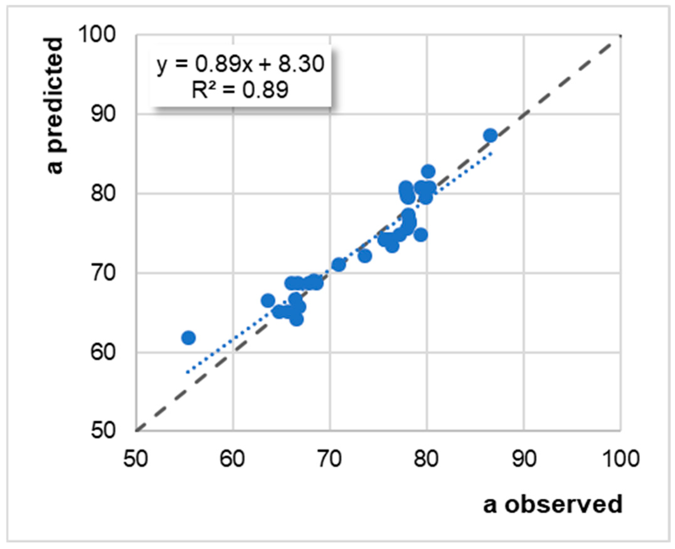
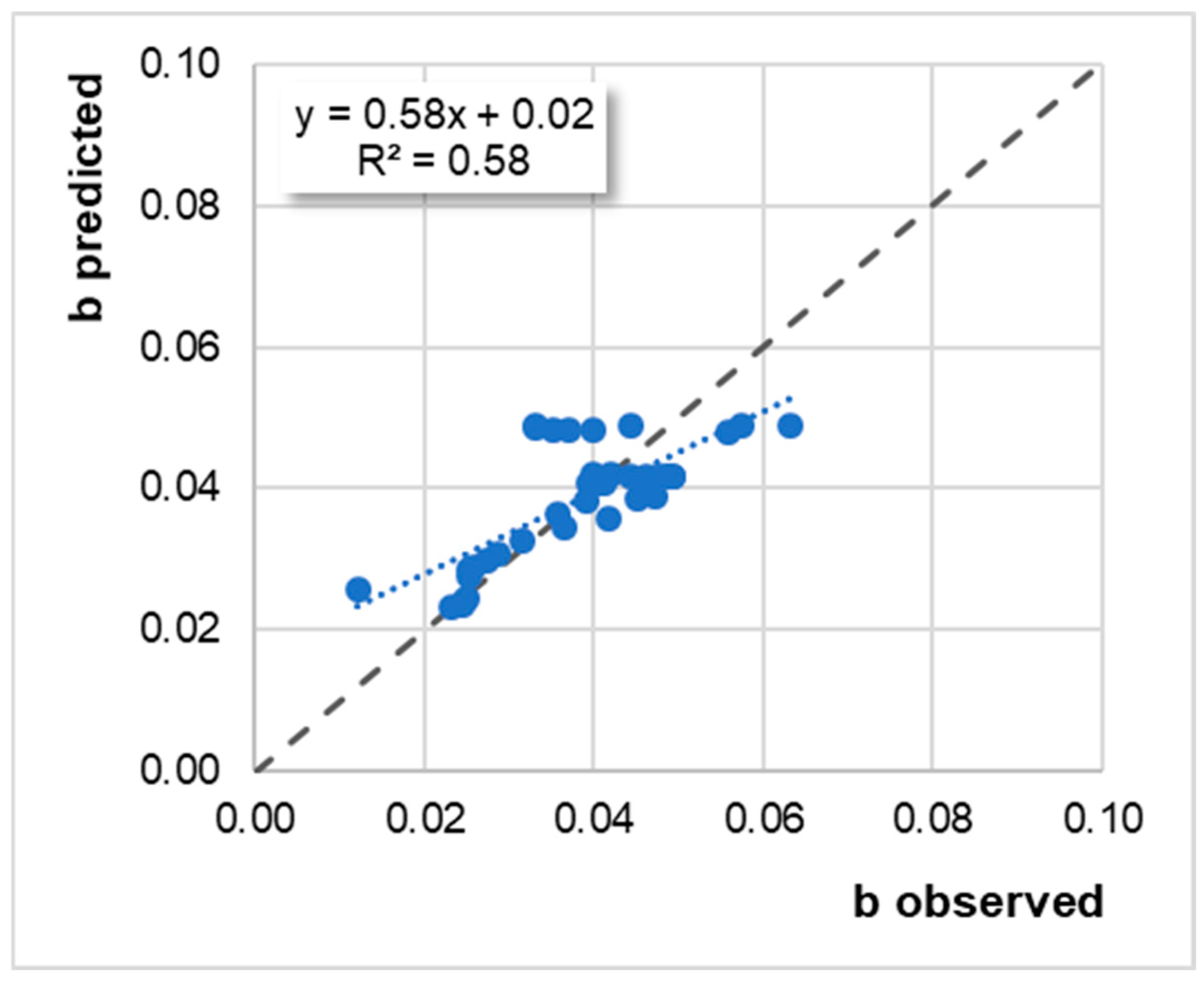
3.2. The Analysis of the Relationship Between the Aggregate Grading and a, b
- The dataset of 22 mixtures produced and tested at UNIRC.
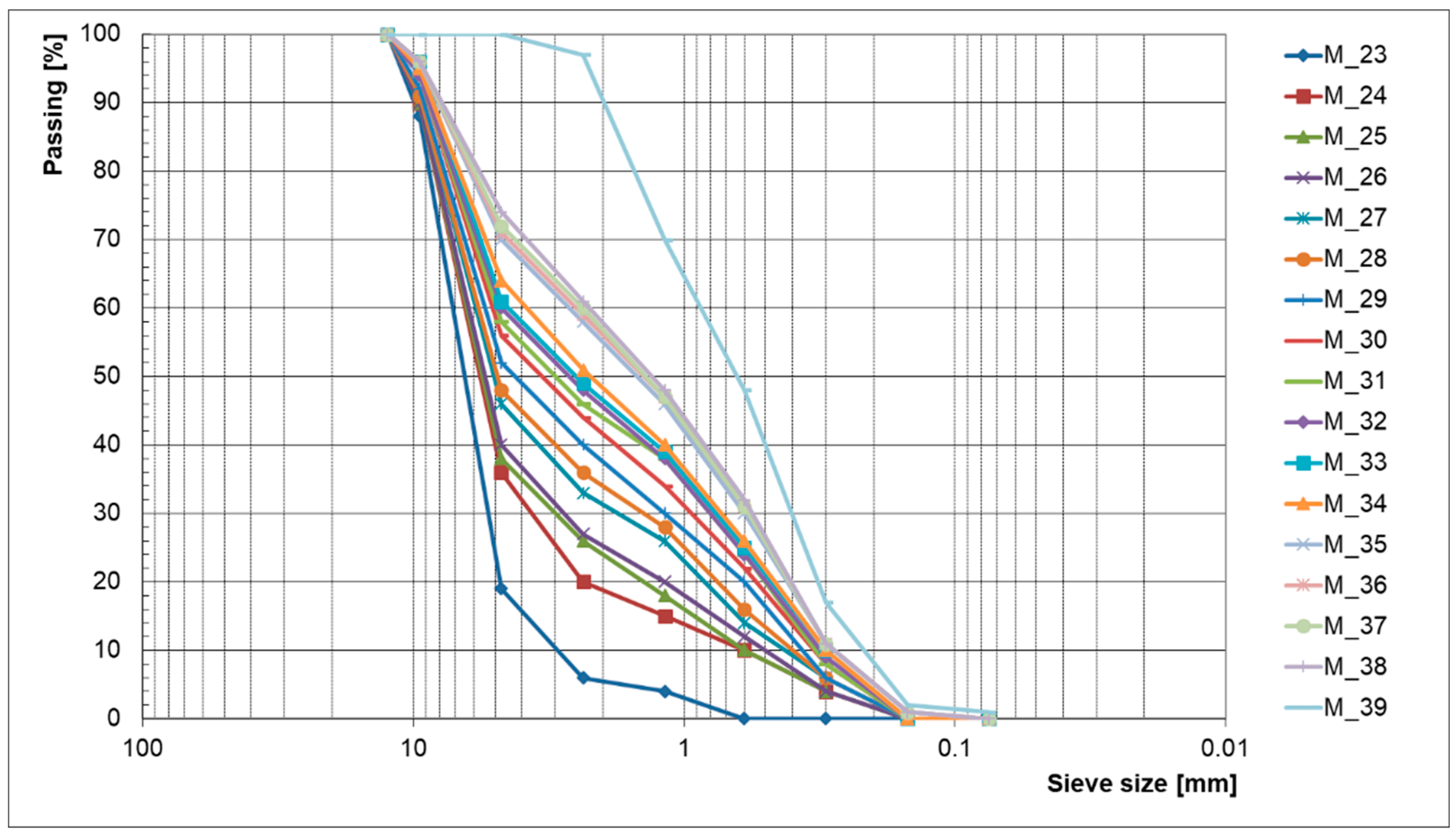
- The dataset of 17 mixtures studied by Pouranian and Haddock [16].
- The dataset of 39 mixtures, including both the sets above.
- There is a strong negative correlation with the squared distance from the maximum density line “dist” (−0.95 for the 17-mixture dataset, −0.90 for the 22-mixture dataset, and −0.80 for all the data). This implies that when the gradation curve deviates more from the maximum density line (i.e., there is a higher squared distance), the initial compaction percentage decreases. This condition translates into a lower initial compaction for poorly graded mixtures. This result reflects the cluster separation (e.g., DG and OG clusters) noted in Section 3.1. Specifically, it is noted that the %Gmm@1 for the DG cluster is higher than that obtained for the OG cluster (77.88% vs. 66.16%).
- There is a positive correlation with the “sand” variable. The coefficients range from 0.63 to 0.93, indicating that as the sand percentage increases, the initial compaction increases as well. The sand content improves the density at early stages.
- For the “dust” variable, a strong positive correlation is recorded for the 22-mixture dataset, while for the entire database, a weak positive correlation is observed. The first value suggests that, for some mixtures, filler can facilitate quicker densification during the early compaction stages.
- As a consequence of the results discussed above, a strong negative correlation was obtained with the coarse aggregate content.
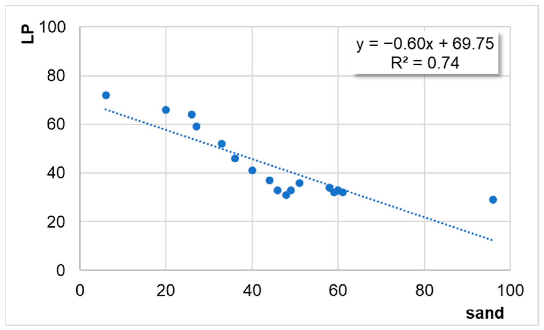
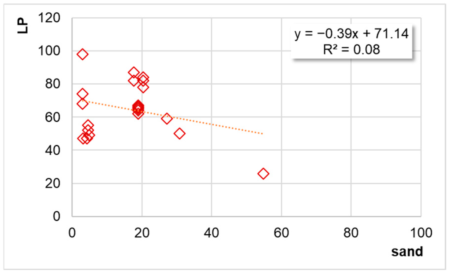
3.3. The Analysis of the Relationship Between the Aggregate Grading and the LP
- Higher sand/fine percentages correspond to lower locking points. Specifically, the regression analysis indicated that sand percentages can explain about 52% of the variance of the LP.
- Higher dust/filler percentages correspond to higher locking points. Dust percentages can explain about 48% of the variance of the LP.
R2 = 0.74
R2 = 0.08
R2 = 0.53
R2 = 0.03
R2 = 0.06
3.4. Regression Model Analysis for LP
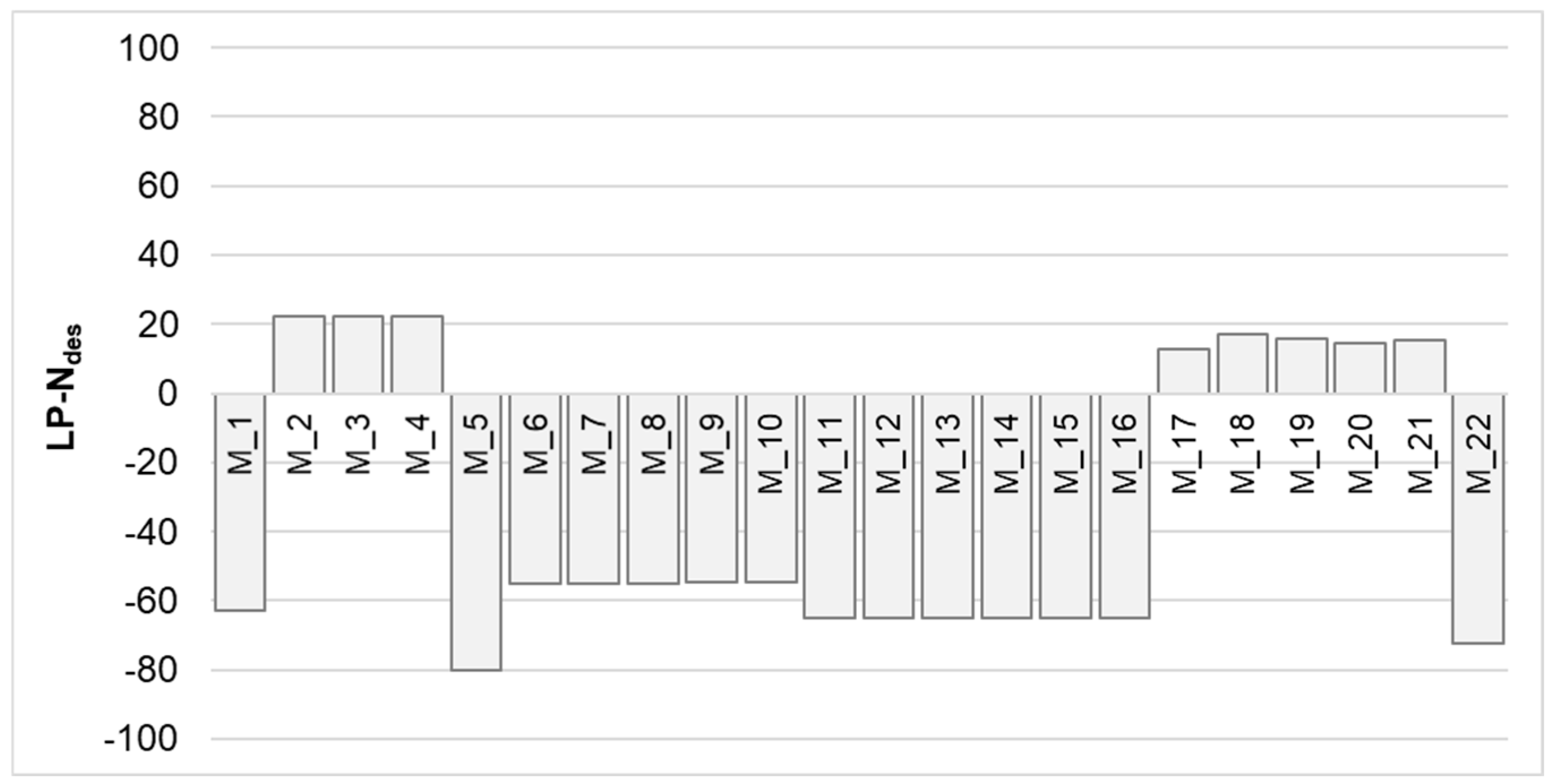
3.5. Analysis of LP-Ndes Data
4. Conclusions
- The laboratory production and testing of 22 mixtures. Furthermore, in order to improve the amount of data, 17 additional mixtures were collected from the literature.
- Define grading-related variables, such as the squared distance from the maximum density line, sand content, dust (or filler) percentage, and coarse aggregate.
- Analyse the relationships between compaction curve parameters and aggregate grading to observe how these factors affect compaction behaviour.
- Develop a regression model to predict the compaction curve parameters based on aggregate grading information.
- Analyse the relationship between aggregate grading and the LP.
- Develop a regression model to predict the LP based on the aggregate gradation.
- Validate the objective function by analysing the LP-Ndes data, where LP refers to the LP predicted and Ndes data refer to contract specifications.
- Derive information on the compaction energy at the laboratory stage by using the predicted compaction curve parameters and the LP (i.e., the assessment of the CDI for each mixture).
- Compaction curves can be modelled through a number of curves. A higher number of parameters allows for a better fit, but attention should also be focused on the intrinsic meaning of parameters and on what happens for very low and very high numbers of gyrations, where the constraints must be considered. The analyses carried out demonstrated that linking the theoretical maximum and the theoretical minimum with the exponents of the curve could lead to a bias between the supposed meaning of the parameter (e.g., maximum %Gmm) and its value as a result of a regression procedure (e.g., 102). The two-parameter and the three-parameter models used herein appeared quite consistent for the cases under analysis.
- Compaction curves can be modelled in terms of the power-law relationship expressed as %Gmm = a·Nb, where “a” represents the initial compaction of the mixture, and the exponent “b” is a measure of the rate of compaction as the number of gyrations increases. From the analyses and the study of the experimental mixtures designed and tested, it was observed that a higher value of the parameter “a” indicates a lower initial AV content, which was identified to be typical of dense-graded mixtures. Specifically, an average AV@1 of 22% was estimated for DG mixtures compared to 34% for OG mixtures. The slightly lower values of “b” recorded for OG mixtures can be associated with a slower compaction “response”, with slopes of approximately 0.06 for OG mixtures compared to 0.08 for DG mixtures.
- New relationships are herein derived to predict compaction curves through composition-related factors. The analysis of the relationship between the compaction curve parameters (a and b) and the aggregate-gradation-related parameters shows how the latter particularly affect the early stage of compaction (i.e., parameter “a”). The most significant correlations are identified between “a” and the squared distance from the maximum density line, indicating that when the gradation curve deviates more from the maximum density line, the initial compaction percentage decreases. This condition translates into a lower initial compaction for poorly graded mixtures. There is also a positive correlation between “a” and the sand content, indicating that as the sand percentage increases, the initial compaction increases as well. Obviously, this condition means that the sand content improves the density at early stages. In contrast, it was found that a higher sand content negatively affects the rate of compaction with increased gyrations. However, the weak correlations observed between “b” and other grading-related variables suggest that other factors, such as the particle shape and the binder, may play a more significant role in influencing compaction at higher gyration levels. For this reason, in future research, attention will be focused on including other mixture-related variables.
- New relationships are herein derived to predict the LP through composition-related factors. Pearson coefficients for the LP vs. grading-related variables show that the most significant correlations with the LP are the sand, filler, and coarse percentages. Higher sand/fine percentages correspond to lower locking points. Specifically, the regression analysis indicates that sand percentages can explain about 52% of the variance of the locking point. In contrast, higher dust/filler percentages correspond to higher locking points. Dust percentages can explain about 48% of the variance of the locking point. The regression model analysis demonstrated that the combined influence of the sand and dust contents explains a significant portion of the variance in the LP.
- On average, LP-Ndes= −34. The analysis of the trend LP-Ndes allows us to confirm the reasonability of the objective function set up herein.
- Aggregate grading control is critical for optimising the compaction process.
- The prediction of the LP at the design stage, based on aggregate-grading-related parameters, allows for better planning and the optimisation of compaction practices.
- The characterisation of the compaction processes allows for the selection of the appropriate compaction equipment at the laboratory stage, which ensures that the compaction energy applied during the construction phase is effective.
- Low-carbon and low-energy strategies and practices can be implemented by optimising the compaction process at the laboratory stage. In fact, the study findings allow for translating lab data into more sustainable on-site compaction practices. It is noteworthy to observe that even with a negligible decrease in terms of the compaction energy, slight increases in the expected life due to the achievement of the correct compaction (e.g., 10%) yield appreciable savings in terms of the environmental impact per year.
- Algorithms allow for the better analysis of competitive equilibria, where competing technologies are compared at the laboratory stage.
- The diversity among the mixtures that were considered (including dense-graded friction courses and open-graded friction courses) suggests that the conclusions above could have quite a wide applicability, and the replicability of the study could be quite high. Anyhow, a higher number of samples and a higher number of compaction-related variables would be needed in order to improve the significance of the findings. Indeed, the analysis should be extended to other mixture-related variables and additional factors to investigate the compaction behaviour of various mixtures better.
- This also applies to the objective function. Future research should explore more mixtures with different gradations and material types, considering the Akaike information criterion (AIC), the Bayesian Information Criterion (BIC), and Cross Validation (CV) for better selecting the best number of parameters.
- The objective function herein set up and the analyses carried out mainly refer to sustainability (energy-related) issues. A broader spectrum of instances should be involved, and the same definition of the objective function emerges as an opportunity for further refinement towards having an objective function that includes more equations.
- The validation of the clustering of mixtures into groups (e.g., OG, DG), the comparison of in-lab and on-site energy densities, and the editing of guidelines for practitioners are supplementary priorities for further research. This also includes finding a parametric way to deal with the issues deriving from the transition from laboratory conditions to on-site conditions (weather conditions, the actual temperatures of mixtures, and the layer thickness).
Author Contributions
Funding
Data Availability Statement
Acknowledgments
Conflicts of Interest
Abbreviations
| SDGs | sustainable development goals |
| LCA | life cycle assessment |
| FAA | fine aggregate angularity |
| CAA | coarse aggregate angularity |
| AV | air void content |
| VMA | voids in mineral aggregate |
| VFA | voids filled with asphalt |
| DG | dense-graded mixes |
| OG | open-graded mixes |
| CEI | compaction energy index |
| LP | locking point |
| CDI | compaction densification index |
| TDI | traffic densification index |
| N | number of gyrations |
| Gmm | theoretical maximum density |
| GER | Global Energy Requirement |
| G | aggregate gradation |
| E | compaction energy |
| CE | competitive equilibrium |
| KPI | key performance indicator |
| SGC | Superpave Gyratory Compactor |
| NMAS | nominal maximum aggregate |
| DGFC | dense-graded friction course |
| PA | porous asphalt |
References
- Praticò, F.G.; Perri, G. A Study on Warm Mix Asphalt Sustainability. In Proceedings of the 10th International Conference on Maintenance and Rehabilitation of Pavements, Guimarães, Portugal, 24–26 July 2024; Pereira, P., Pais, J., Eds.; Springer Nature: Cham, Switzerland, 2024; pp. 284–292. [Google Scholar]
- Praticò, F.G.; Perri, G. Are Low-Temperature Asphalts a Good Choice? In Proceedings of the Pavement, Roadway, and Bridge Life Cycle Assessment 2024, Arlington, VA, USA, 6–8 June 2024; Flintsch, G.W., Amarh, E.A., Harvey, J., Al-Qadi, I.L., Ozer, H., Lo Presti, D., Eds.; Springer Nature: Cham, Switzerland, 2024; pp. 99–106. [Google Scholar]
- Zhao, Y.; Xie, S.; Gao, Y.; Zhang, Y.; Zhang, K. Prediction of the Number of Roller Passes and Degree of Compaction of Asphalt Layer Based on Compaction Energy. Constr. Build. Mater. 2021, 277, 122274. [Google Scholar] [CrossRef]
- Praticò, F.G.; Perri, G.; De Rose, M.; Vaiana, R. Comparing Bio-Binders, Rubberised Asphalts, and Traditional Pavement Technologies. Constr. Build. Mater. 2023, 400, 132813. [Google Scholar] [CrossRef]
- Wang, X.; Duan, Z.; Wu, L.; Yang, D. Estimation of Carbon Dioxide Emission in Highway Construction: A Case Study in Southwest Region of China. J. Clean. Prod. 2015, 103, 705–714. [Google Scholar] [CrossRef]
- Bijleveld, F.R.; Miller, S.R.; De Bondt, A.H.; Dorée, A.G. Aligning Laboratory and Field Compaction Practices for Asphalt—The Influence of Compaction Temperature on Mechanical Properties. Int. J. Pavement Eng. 2016, 17, 727–740. [Google Scholar] [CrossRef]
- Bertulienė, L.; Augutis, A. Experimental Study for Asphalt Laying Using Control of Pavement Compaction Technology on Roads. In Proceedings of the 10th International Conference Environmental Engineering, Vilnius, Lithuania, 27–28 April 2017. [Google Scholar] [CrossRef]
- Polaczyk, P.; Han, B.; Gong, H.; Ma, Y.; Xiao, R.; Hu, W.; Huang, B. Influence of Aggregate Gradation on the Compactability of Asphalt Mixtures Utilizing Locking Point. J. Mater. Civ. Eng. 2021, 33, 04021005. [Google Scholar] [CrossRef]
- Polaczyk, P.; Ma, Y.; Hu, W.; Xiao, R.; Jiang, X.; Huang, B. Effects of Mixture and Aggregate Type on Over-Compaction in Hot Mix Asphalt in Tennessee. Transp. Res. Rec. 2022, 2676, 448–460. [Google Scholar] [CrossRef]
- Mahmoud, A.F.F.; Bahia, H. Using Gyratory Compactor to Measure Mechanical Stability of Asphalt Mixtures; Wisconsin Highway Research Program: Portage, WI, USA, 2004. [Google Scholar]
- Mohammad, L.; Shamsi, K. A Look at the Bailey Method and Locking Point Concept in Superpave Mixture Design. Transp. Res. Circ. 2007, EC-124, 24–32. [Google Scholar]
- AASHTO. American Association of State Highway and Transportation Officials (AASHTO) AASHTO Provisional Standards, April 2001 Interim Edition; AASHTO: Washington, DC, USA, 2000. [Google Scholar]
- Airey, G.D.; Collop, A.C. Mechanical and Structural Assessment of Laboratory- and Field-Compacted Asphalt Mixtures. Int. J. Pavement Eng. 2016, 17, 50–63. [Google Scholar] [CrossRef]
- Bahia, H.U.; Friemel, T.P.; Peterson, P.A.; Russell, J.S.; Poehnelt, B. Optimization of Constructibility and Resistance to Traffic: A New Design Approach for HMA Using the Superpave Compactor. J. Assoc. Asph. Paving Technol. 1998, 67, 189–232. [Google Scholar]
- Mikhailenko, P.; Griffa, M.; Pieren, R.; Pachale, U.; Poulikakos, L.D. Pore Space of In-Situ Semi-Dense Asphalt: A Characterization by X-Ray Tomography. Constr. Build. Mater. 2024, 453, 139091. [Google Scholar] [CrossRef]
- Pouranian, M.R.; Haddock, J.E. A New Framework for Understanding Aggregate Structure in Asphalt Mixtures. Int. J. Pavement Eng. 2021, 22, 1090–1106. [Google Scholar] [CrossRef]
- Leiva, F.; West, R.C. Analysis of Hot-Mix Asphalt Lab Compactability Using Lab Compaction Parameters and Mix Characteristics. Transp. Res. Rec. 2008, 2057, 89–98. [Google Scholar] [CrossRef]
- ANAS S.p.A. Capitolato Speciale Di Appalto. In Norme Tecniche per l’esecuzione Del Contratto Parte 2. Pavimentazioni Stradali; ANAS S.p.A.: Rome, Italy, 2016. [Google Scholar]
- Ministero dei Lavori Pubblici CIRS. Centro Sperimentale Interuniversitario Di Ricerca Stradale. Capitolato Speciale d’appalto Tipo per Lavori Stradali; Ministero dei Lavori Pubblici: Rome, Italy, 2001.
- Caputo, P.; Calandra, P.; Vaiana, R.; Gallelli, V.; De Filpo, G.; Rossi, C.O. Preparation of Asphalt Concretes by Gyratory Compactor: A Case of Study with Rheological and Mechanical Aspects. Appl. Sci. 2020, 10, 8567. [Google Scholar] [CrossRef]
- Vavrik, W.R.; Carpenter, S.H. Calculating Air Voids at Specified Number of Gyrations in Superpave Gyratory Compactor. Transp. Res. Rec. 1998, 1630, 117–125. [Google Scholar] [CrossRef]
- Polaczyk, P.; Huang, B.; Shu, X.; Gong, H. Investigation into Locking Point of Asphalt Mixtures Utilizing Superpave and Marshall Compactors. J. Mater. Civ. Eng. 2019, 31, 04019188. [Google Scholar] [CrossRef]
- Cheng, Z.; Jia, X.; Jiang, H.; Hu, W.; Huang, B. Quantification of Impact Compaction Locking Point for Asphalt Mixture. Constr. Build. Mater. 2021, 302, 124410. [Google Scholar] [CrossRef]
- Poulikakos, L.D.; Pasquini, E.; Tusar, M.; Hernando, D.; Wang, D.; Mikhailenko, P.; Pasetto, M.; Baliello, A.; Cannone Falchetto, A.; Miljković, M.; et al. RILEM Interlaboratory Study on the Mechanical Properties of Asphalt Mixtures Modified with Polyethylene Waste. J. Clean. Prod. 2022, 375, 134124. [Google Scholar] [CrossRef]
- Mocelin, D.M.; Brito, L.A.T.; Johnston, M.G.; Alves, V.S.; Colpo, G.B.; Ceratti, J.A.P. Evaluation of Workability of Warm Mix Asphalt through Cdi Parameter and Air Voids. Transport Infrastructure and Systems. In Proceedings of the AIIT International Congress on Transport Infrastructure and Systems, TIS 2017, Rome, Italy, 10–12 April 2017; pp. 335–341. [Google Scholar] [CrossRef]
- Huang, J.; Kumar, G.S.; Sun, Y. Evaluation of Workability and Mechanical Properties of Asphalt Binder and Mixture Modified with Waste Toner. Constr. Build. Mater. 2021, 276, 122230. [Google Scholar] [CrossRef]
- Sanchez-Alonso, E.; Vega-Zamanillo, A.; Castro-Fresno, D.; Delrio-Prat, M. Evaluation of Compactability and Mechanical Properties of Bituminous Mixes with Warm Additives. Constr. Build. Mater. 2011, 25, 2304–2311. [Google Scholar] [CrossRef]
- Yu, S.; Shen, S.; Lu, M. Data Sensing and Compaction Condition Modeling for Asphalt Pavements. Autom. Constr. 2023, 154, 105021. [Google Scholar] [CrossRef]
- Dan, H.; Li, S.; Chen, J.; Li, W. Dynamic Response and Compaction Evaluation of Asphalt Pavement in Different Infrastructure Types through an Energy-Based Approach. Constr. Build. Mater. 2025, 479, 141501. [Google Scholar] [CrossRef]
- Shan, H.; Dan, H.-C.; Wang, S.; Zhang, Z.; Zhang, R.; Shan, H.; Dan, H.-C.; Wang, S.; Zhang, Z.; Zhang, R. Investigation on Dynamic Response and Compaction Degree Characterization of Multi-Layer Asphalt Pavement under Vibration Rolling. Electron. Res. Arch. 2023, 31, 2230–2251. [Google Scholar] [CrossRef]
- Praticò, F.G.; Fedele, R.; Pellicano, G. Pavement FRFs and Noise: A Theoretical and Experimental Investigation. Constr. Build. Mater. 2021, 294, 123487. [Google Scholar] [CrossRef]
- Moutier, F. Modelisation Des Resultats de La Pcg Reflexions a Propos Du Seuil Ultime de Compactage. In Proceedings of the Eurasphalt & Eurobitume Congress, Strasbourg, France, 7–10 May 1996; pp. 7–10. [Google Scholar]
- Margaritis, A.; Tanghe, T.; De Visscher, J.; Vansteenkiste, S.; Vanelstraete, A. The Use of Gyratory Compaction to Assess the Workability of Asphalt Mixtures. In Green and Intelligent Technologies for Sustainable and Smart Asphalt Pavements, Proceedings of the 5th International Symposium on Frontiers of Road and Airport Engineering IFRAE, Delft, The Netherlands, 12–14 July 2021; CRC Press: London, UK, 2022; pp. 91–97. [Google Scholar]
- Gao, Y.; Huang, X.; Yu, W. The Compaction Characteristics of Hot Mixed Asphalt Mixtures. J. Wuhan Univ. Technol. Mater. Sci. Ed. 2014, 29, 956–959. [Google Scholar] [CrossRef]
- Stakston, A.D.; Bahia, H.U.; Bushek, J.J. Effect of Fine Aggregate Angularity on Compaction and Shearing Resistance of Asphalt Mixtures. Transp. Res. Rec. J. Transp. Res. Board 2002, 1789, 14–24. [Google Scholar] [CrossRef]
- Praticò, G.F.; Fedele, R. Road Pavement Macrotexture Estimation at the Design Stage. Constr. Build. Mater. 2023, 364, 129911. [Google Scholar] [CrossRef]
- Bezdek, K.; Khan, M.A. Contact Numbers for Sphere Packings. Bolyai Soc. Math. Stud. 2018, 27, 25–47. [Google Scholar] [CrossRef]


| N = 1 | N = 8 | Nini | N@92%Gmm | Ndes | LP | N@98%Gmm | Nmax | |
|---|---|---|---|---|---|---|---|---|
| (*) | (**) | 6–10 (***) | 50–140 | 30–100 | (****) | 75–230 | ||
| Constraints | AV@Nini | AV@Ndes, VMA@Ndes, VFA@Ndes | Δh | AV@Nmax | ||||
| Energy-related indicators | CEI | |||||||
| CDI | ||||||||
| TDI | ||||||||
| Mixture ID | b [%] | NMAS [mm] | Tmix [°C] | Ndes |
|---|---|---|---|---|
| M_1 | 5.56 | 9.8 | 180 | 130 |
| M_2 | 4.20 | 14.8 | 180 | 50 |
| M_3 | 4.20 | 14.8 | 180 | 50 |
| M_4 | 4.80 | 12.8 | 180 | 50 |
| M_5 | 6.31 | 5.8 | 140 | 130 |
| M_6 | 6.98 | 7.2 | 180 | 130 |
| M_7 | 6.98 | 7.2 | 180 | 130 |
| M_8 | 6.98 | 7.2 | 180 | 130 |
| M_9 | 6.98 | 7.3 | 180 | 130 |
| M_10 | 7.24 | 7.1 | 180 | 130 |
| M_11 | 6.35 | 7.0 | 140 | 130 |
| M_12 | 6.35 | 7.0 | 140 | 130 |
| M_13 | 6.35 | 7.0 | 140 | 130 |
| M_14 | 6.35 | 7.0 | 140 | 130 |
| M_15 | 6.35 | 7.0 | 140 | 130 |
| M_16 | 6.35 | 7.0 | 140 | 130 |
| M_17 | 4.83 | 14.2 | 160 | 50 |
| M_18 | 4.70 | 14.2 | 160 | 50 |
| M_19 | 3.91 | 14.0 | 160 | 50 |
| M_20 | 3.83 | 14.3 | 160 | 50 |
| M_21 | 4.85 | 13.9 | 160 | 50 |
| M_22 | 4.97 | 14.5 | 180 | 130 |
| Parameters/Outputs | M_3 | M_4 | M_22 | |
|---|---|---|---|---|
| Power law: | a | 68.63 | 64.48 | 79.33 |
| b | 0.06 | 0.05 | 0.04 | |
| %Gmm@0 | - | - | - | |
| %Gmm@8 | 77.33 | 71.60 | 86.07 | |
| %Gmm@Ndes | 85.91 | 78.53 | 96.01 | |
| %Gmm@∞ | 121.17 | 106.22 | 116.97 | |
| Logarithm law: | c | 4.84 | 3.90 | 3.58 |
| d | 67.16 | 63.43 | 78.57 | |
| %Gmm@0 | NA | NA | NA | |
| %Gmm@8 | 77.23 | 71.53 | 86.02 | |
| %Gmm@Ndes | 86.11 | 78.67 | 96.00 | |
| %Gmm@∞ | 115.14 | 102.01 | 114.03 | |
| Three-parameter quotient: | h | 2638.41 | 2389.59 | 2787.04 |
| l | 96.19 | 86.69 | 99.83 | |
| m | 36.51 | 35.44 | 33.96 | |
| %Gmm@0 | 72.27 | 67.42 | 82.06 | |
| %Gmm@8 | 76.57 | 70.97 | 85.45 | |
| %Gmm@Ndes | 86.10 | 78.69 | 96.15 | |
| %Gmm@∞ | 96.15 | 86.65 | 99.80 | |
| Moutier model | C0 | 53.48 | 48.14 | 62.06 |
| C∞ | 111.47 | 119.21 | 130.97 | |
| b3 | 0.01 | 0.00 | 0.00 | |
| b4 | 0.33 | 0.30 | 0.34 | |
| %Gmm@0 | 53.48 | 48.14 | 62.06 | |
| %Gmm@8 | 76.87 | 71.54 | 86.02 | |
| %Gmm@Ndes | 86.07 | 78.55 | 96.02 | |
| %Gmm@∞ | 106.38 | 101.29 | 113.19 | |
| Moutier model where C∞ is constrained (C∞ ≤ 100%) | C0 | 69.99 | 51.21 | 79.86 |
| C∞ | 100.00 | 100.00 | 100.00 | |
| β3 | 0.02 | 0.01 | 0.04 | |
| β4 | 2867.66 | 0.35 | 0.06 | |
| %Gmm@0 | 69.99 | 51.21 | 79.86 | |
| %Gmm@8 | 99.99 | 71.39 | 85.37 | |
| %Gmm@Ndes | 100.00 | 78.72 | 95.98 | |
| %Gmm@∞ | 100.00 | 95.30 | 99.93 |
| Mixture ID | a | b |
|---|---|---|
| M_1 | 80.16 | 0.04 |
| M_2 | 67.91 | 0.06 |
| M_3 | 68.63 | 0.06 |
| M_4 | 66.70 | 0.04 |
| M_5 | 86.56 | 0.01 |
| M_6 | 80.33 | 0.04 |
| M_7 | 79.42 | 0.04 |
| M_8 | 79.50 | 0.04 |
| M_9 | 78.11 | 0.04 |
| M_10 | 79.86 | 0.04 |
| M_11 | 75.61 | 0.05 |
| M_12 | 76.37 | 0.05 |
| M_13 | 76.24 | 0.05 |
| M_14 | 75.74 | 0.05 |
| M_15 | 76.08 | 0.05 |
| M_16 | 75.63 | 0.04 |
| M_17 | 66.54 | 0.03 |
| M_18 | 66.41 | 0.04 |
| M_19 | 65.70 | 0.03 |
| M_20 | 64.79 | 0.04 |
| M_21 | 66.84 | 0.04 |
| M_22 | 79.33 | 0.04 |
| Parameter | Group | |||
|---|---|---|---|---|
| OG | Intermediate | DG | M5 | |
| a | 66.16 | 68.27 | 77.88 | 86.56 |
| b | 0.037 | 0.060 | 0.043 | 0.012 |
| %Gmm@1 | 66.16 | 68.27 | 77.88 | 86.56 |
| AV@1 [%] | 34 | 32 | 22 | 13 |
| y′@1 | 2.46 | 4.12 | 3.37 | 1.06 |
| %Gmm@50 | 76.51 | 86.45 | 92.26 | 90.79 |
| AV@50 [%] | 23 | 14 | 7 | 9 |
| y′@50 | 0.06 | 0.10 | 0.08 | 0.02 |
| Parameter of the Compaction Curve | Dataset | Aggregate-Grading-Related Variables | |||
|---|---|---|---|---|---|
| Dist | Sand | Dust | Coarse | ||
| a | 17 mixtures | −0.95 | 0.93 | - | −0.93 |
| 22 mixtures | −0.90 | 0.91 | 0.71 | −0.91 | |
| 17 + 22 mixtures | −0.80 | 0.63 | 0.32 | −0.63 | |
| b | 17 mixtures | 0.85 | −0.97 | - | 0.97 |
| 22 mixtures | 0.08 | −0.52 | 0.06 | 0.52 | |
| 17 + 22 mixtures | 0.38 | −0.76 | 0.34 | 0.76 | |
| Regression Coefficients | |||||
|---|---|---|---|---|---|
| a | b | ||||
| β1 | β2 | β3 | β4 | β5 | β6 |
| 0.34 | 1.33 | 59.70 | −4.5 × 10⁻⁴ | −5.0 × 10⁻⁵ | 0.05 |
| Grading-Related Variables | r | |
|---|---|---|
| Pi | 20 | 0.26 |
| 16 | −0.03 | |
| 12.5 | −0.15 | |
| 9.5 | −0.15 | |
| 4.75 | −0.46 | |
| 2.36 | −0.65 | |
| 1.18 | −0.66 | |
| 0.6 | −0.63 | |
| 0.3 | −0.04 | |
| 0.15 | 0.61 | |
| 0.075 | 0.69 | |
| dist | 0.24 | |
| sand | −0.72 | |
| dust | 0.69 | |
| coarse | 0.72 | |
| 17-Mixture Dataset | 22-Mixture Dataset | 39-Mixture Dataset | |
|---|---|---|---|
| A | −0.84 | −0.89 | −0.45 |
| B | 31.03 | 5.35 | 2.27 |
| C | 78.72 | 44.61 | 59.93 |
| R2 | 0.90 | 0.70 | 0.69 |
Disclaimer/Publisher’s Note: The statements, opinions and data contained in all publications are solely those of the individual author(s) and contributor(s) and not of MDPI and/or the editor(s). MDPI and/or the editor(s) disclaim responsibility for any injury to people or property resulting from any ideas, methods, instructions or products referred to in the content. |
© 2025 by the authors. Licensee MDPI, Basel, Switzerland. This article is an open access article distributed under the terms and conditions of the Creative Commons Attribution (CC BY) license (https://creativecommons.org/licenses/by/4.0/).
Share and Cite
Praticò, F.G.; Perri, G. The Prediction of the Compaction Curves and Energy of Bituminous Mixtures. Infrastructures 2025, 10, 132. https://doi.org/10.3390/infrastructures10060132
Praticò FG, Perri G. The Prediction of the Compaction Curves and Energy of Bituminous Mixtures. Infrastructures. 2025; 10(6):132. https://doi.org/10.3390/infrastructures10060132
Chicago/Turabian StylePraticò, Filippo Giammaria, and Giusi Perri. 2025. "The Prediction of the Compaction Curves and Energy of Bituminous Mixtures" Infrastructures 10, no. 6: 132. https://doi.org/10.3390/infrastructures10060132
APA StylePraticò, F. G., & Perri, G. (2025). The Prediction of the Compaction Curves and Energy of Bituminous Mixtures. Infrastructures, 10(6), 132. https://doi.org/10.3390/infrastructures10060132