The Phasor Diagram of a Superconducting Synchronous Electrical Machine

Abstract

This paper describes a universal method proposed by the author for the evaluative analytical calculation of the main parameters of synchronous electrical machines, including superconducting ones. Traditional methods for analytical calculation of parameters to build a phasor diagram of electrical machines require a calculation of all dimensions of the active zone, tooth-slot zone and frontal parts of armature windings. All sizes and local states of magnetic circuit saturation are necessary for the calculation of magnetic conductivities. Traditional analytical methods use, among other things, empirical formulas and non-physical coefficients and allow one to calculate only standard machines with classic tooth-slot zones and armature winding types. As a result of drawing a phasor diagram using traditional methods, the angle between the electromotive force and voltage is calculated, which is the machine’s internal parameter and has no major significance for users. The application of modern computer programs for simulation requires a preliminary analytical calculation in order to obtain all dimensions of the three-dimensional model. FEM simulation programs are expensive, require expensive high-performance computers and highly paid skilled personnel. Fast analytical techniques are also required to assess the correctness of the obtained automatic computer simulation results. The proposed analytical method makes it possible to quickly obtain all the main parameters of a newly designed machine (including superconducting ones and those of non-traditional design) without a detailed calculation of the dimensions of the tooth-slot zone and armature end-windings. The characteristic values of load angles are set according to the results of simple calculations, and the desired values, obtained via plotting, represent the inductive resistances of armature winding and inductive voltage drop across it. Results of practical significance, calculated from the voltage diagram, are as follows: the inductor’s magnetomotive force necessary to maintain the nominal load voltage value, regardless of the magnitude (including double overload) and type of the connected load, or the main dimensions of the active zone.

1. Introduction

Currently, well-known computer simulation software products are used for automated calculations of synchronous electrical machines. A necessary preliminary stage of computer simulation is to obtain a detailed design sketch of the machine geometry, the dimensions for which are calculated as a result of analytical calculation using well-known or modified methods. However, the proven calculation methods of large corporations for the design of mass-produced machines may be a trade secret. Textbooks for students, usually, do not contain ready-made calculation methods, explaining only operation principles and parameter relationship instead. For electrical machines of well-known types, the search for an analytical calculation method for specialist engineers is not difficult. However, for electrical machines of new types or with non-traditional elements in the active zone, the known methods cannot be directly applied without appropriate modifications. Thus, there is a need for a universal method for carrying out at least preliminary evaluative calculations, with accurate assumptions and minor simplifications made, based on traditional graph-analytical methods and simple well-known equation laws. Operation principles and the relationship of main parameters of any synchronous electrical machine are illustrated by diagrams developed by electrical engineers of the late 19th and early 20th centuries, among which, special mention should be made of the contribution of Andre Potier, Andre Blondel, Hans Behn-Eshenburg [1,2], A. Rothert, Engelbert Arnold [3].

Phasor diagram of an electrical machine clearly shows the relationship of all its main electromagnetic and electrical parameters. The voltage diagram, also often erroneously referred to as vector diagram, formerly had the traditional “phasor diagram” name. It is a set of segments (radius vectors) with a length corresponding to the displayed value, symbolizing the relative angular shift in time of cyclic electromagnetic processes occurring in an alternating current (AC) electric machine. Segment directions conditionally show the mutual influence (strengthening or weakening) of values of similar physical essence and dimension.

Traditionally, phasor diagrams, without observing dimensions and scales, are schematically used only to demonstrate the operating principles of AC electrical machines and their modes of operation. More rarely, a reporting diagram is built to visually illustrate the results of a particular machine calculation. After the compilation of canonical [1,2] phasor diagrams at the turn of the 19th and 20th centuries, geometrically visualized parameter relationships were mathematically described [4,5]. Analytical calculation methods were compiled from those formulas. Analytical methods were algorithmized with the development of computer technologies, and as a result, computer software for automated calculation was developed. As an example of a perspective technique, one can consider a recently developed approach to power analysis [6,7] which is exploiting cyclostationary properties [8,9] of voltage and current signals. Such an approach can mitigate the arbitrary periodic excitation which may be chosen as a possible way to further improve the tool presented in this paper. However, its practical implementation will inevitably require an increase in the amount of the required computational resources, as shown in [10], where a practical prototype is introduced. The recently established trend raises concern that programs will automatically calculate electrical machines without any significant human participation at each step in the future. At the same time, engineers, without understanding the theoretical basis and general operating principles without any methodological tools independent of computers, will not be able to assess the correctness of the results they obtain. The ability to apply fundamental physical laws in practice is a necessary competence of any engineer. Primary literature printed about a hundred years ago and published in relatively small number of copies has become a hard-to-reach bibliographic rarity by now. This paper will be useful for students trying to understand and engineers willing to refresh the principles of how AC electrical machines work; it will help them build analytical algorithms for the required calculations. With a solid understanding of these principles, they will be able to develop their own methods for newly designed machines.

The main difficulty in calculating the parameters of new types of electrical machines is the calculation of synchronous inductive resistance. Inductive reactance causes a voltage drop across the generator due to the armature reaction phenomenon. The calculation includes the assessment of armature winding inductance and leakage flux inductance [11,12,13,14]. Usually, the active resistance of the armature winding is much less than the inductive resistance and does not have a significant effect on the voltage drop, especially in superconducting windings. Designing a new machine, it is necessary to ensure that its real characteristics correspond to the specified parameters. The most important parameters are rated power and voltage. Without a correct calculation of voltage drop, due to the influence of synchronous inductive reactance, the machine will not provide the rated generator’s voltage under load and when overloaded. Additionally, it will also not deliver the rated power. Small errors in calculation can be compensated for by an increase in the excitation current during operation; however, this will lead to an increase in losses, decrease in efficiency and the risk of emergency thermal damage to winding insulation. When the generator is excited by permanent magnets, an error in calculation of synchronous inductive resistance will inevitably lead to a voltage mismatch with the nominal value in the operating mode. Resizing the inductor will lead to an unjustified increase in the machine’s dimensions and weight.

Traditional and modern methods involve a laborious approximate analytical calculation of magnetic conductivities to calculate armature winding inductances. The calculation of magnetic conductivities of standard machines is possible only after obtaining all the dimensions of the active zone, tooth-slot zone and armature end-windings. The finite element method (FEM) simulation also implies the availability of a calculated geometry with all dimensions.

Thus, the correct calculation is a labor-intensive iterative process, with time expenditure depending on computer system performance and staff qualifications.

At the first stage, it is necessary to calculate the active zone dimensions, which is carried out with the use of the main calculation equation. By introducing the values of cosines of operating angles into this equation, it is possible to increase the size of the active zone to compensate for the voltage drop across the synchronous inductive resistance.

There is often a need for a quick evaluative calculation of a conventional electrical machine of a known type being designed. In this case, time-consuming analytical and FEM simulations are not suitable. At subsequent stages, the obtained estimated parameters can be adjusted in the process of a full iterative calculation with verification using an FEM simulation.

Another area of application of the proposed methodology is a quick assessment of the correctness of the obtained results. These include results obtained by subcontractors, computer programs for automatic calculation, innovative methods, as well as student reports.

All the existing analytical techniques are overly complicated and are becoming increasingly complex without adding any measurable accuracy. Their practical application, as a method for calculating new electrical machines, is extremely difficult. The combination of all these reasons can cause a stagnation and systemic crisis, which will hamper the development of new types of electric machines with a high specific and operational performance.

Most of the well-known authors draw a highly simplified diagram that does not include MMF (or magnetic fluxes) triangles. A minority of authors draw attention to the relationship between MMF and the induced EMF, but do not focus on the approximate similarity of MMF and EMF triangles. None of the authors propose using this similarity to create an algorithm for the evaluative calculation of all the main parameters of the electric machine. The key elements of phasor diagrams drawn by the reviewed authors are summarized in

Table 1. Page numbers of the available publications with their key elements.

Author	EMF on the Diagram	MMF and EMF on the Diagram	Similarity of EMF and MMF	Calculation of Flux Leakage Algorithm	Simple Algorithm
[11]	-	372–383	-	230–253	-
[12]	-	-	-	370–379	-
[13]	-	-	-	98–128	-
[14]	130, 193, 407	-	-	141–145	-
[15]	168–170	-	-	-	-
[16]	550, 600–602	570–573	-	-	-
[17]	206	200	177	-	-
[18]	9, 171	136	-	-	-
[19]	377	144	476	-	-
[20]	244	-	-	-	-
[21]	164–167	-	-	-	-
[22]	300	-	-	-	-
[23]	577–582	-	-	-	-
[24]	49	-	-	-	-
[25]	135–152	-	-	-	-

.

The novelty of the proposed methodology for evaluative calculation of the developed synchronous electrical machine parameters lies in the absence, at the first stage, of the need for a detailed calculation of:

• rotor and stator magnetic circuits;
• magnetic conductivities of scattering;
• armature winding inductive resistance;
• tooth-slot zone dimensions;
• armature end-windings.

A new version of the main calculation equation is presented, which takes into account the nominal working angles and the expected efficiency. A new universal algorithm is suggested for drawing a phasor diagram for a synchronous electric generator of any type, including superconducting generators with combined excitation. The presented algorithm can be easily modified to calculate a synchronous electric motor, such as a brushless DC motor.

2. Materials and Methods

2.1. The Main Parameters of Phasor Diagram

Segments with a conditional direction, called vectors for simplicity, that radiate from the center 0 are radius vectors. However, for convenience, their additions and subtractions can be moved in parallel to the end of other vectors while maintaining the original magnitude, direction, and slope. Vectors’ direction can also be changed by adding a minus sign before the designation of the physical value. For example, for motoring mode, we can reduce the size of the diagram by placing the vectors more compactly in one half-plane.

All vectors rotate cyclically in a positive direction (counterclockwise) around the center of the diagram 0 with angular frequency $\omega =2\cdot \pi \cdot f$, where $f$ is the electrical frequency associated with rotor mechanical speed, measured in RPM using the following formula:

$$f=p\cdot \raisebox{1ex}{$n$}\!\left/ \!\raisebox{-1ex}{$60$}\right.,$$

(1)

where $p$ is the number of pole pairs. Here, and below, the divisor 60 is present in the formulas to convert revolutions per minute to the SI system—revolutions per sec. Angles between vectors are called electrical angles and are measured in electrical degrees. Traditional physical angles have no direction; however, for the convenience of addition and subtraction, as for the vectors in the diagram, the positive direction, for generator mode, is a counterclockwise direction. We can convert the angle between vectors into their time shift (delay in seconds) for a particular machine by multiplying the angle value by $\frac{1}{\Omega \cdot p}.$, where $\Omega$ is the angular frequency of rotor rotation:

$$\Omega =2\cdot \pi \cdot \raisebox{1ex}{$n$}\!\left/ \!\raisebox{-1ex}{$60$}\right..$$

(2)

There are numerous common options for the location of the base axis of the diagram: voltage U upwards [15,26,27]; voltage U to the right [16]; the most popular is EMF E upwards and longitudinal axis d horizontally [17,18,19,20,21,28,29,30]; EMF E to the right [22]; armature phase current I upwards [23,31]; armature phase current I to the right [30,31,32]. The traditional option, also used in this paper, is the “current to the right.” Since the main angles are related to the axis accommodating load current I (also known as armature winding phase current I_a), network load voltage U_L, armature reaction flux Φ_a, and magnetomotive force (MMF) of the armature reaction F_a, it will be more convenient to make projections on it when it is horizontal in programs for analytical calculation and plotting. On the complex plane, the horizontal axis of the current is real—Re—and the vertical axis is imaginary—Im.

Of the two non-collinear vectors forming the angle, the one located in a more counterclockwise direction is the leading one, and the more clockwise one is lagging behind it.

The main physical parameters of the diagram are electromotive forces E (EMF), voltages U and voltage drop, measured in volts. Additional parameters are magnetomotive forces F (MMF) and currents I, measured in amperes. For electrical machines with resistive windings, for proportionality on a single diagram of MMF vectors to EMF vectors, it is more convenient to designate F in deciampereturns (dAt), and in hectaampereturns (hAt) for superconducting windings. The often-used phasor diagram without an MMF (or flux) diagram is not complete. The diagram proposed by Potier, which includes both voltages and MMF, fully describes the spatio-temporal and cause-and-effect interaction of magnetic and electrical parameters of the electric machine. Voltages and currents are recorded in effective (RMS) values [7]. The voltage is phase to neutral, the full armature current flows through the phase of the armature winding (AW) and through the load connected to the machine terminals (for the generator) or the power supply (for the motor). Sometimes, the diagrams display magnetic fluxes Φ, corresponding to MMF in directions and designations, but taking into account magnetic resistances. For the convenience of calculations, it is recommended to indicate scales on the reporting diagram, for example, “1:4 hAt/mm”. By measuring the length of the MMF vector using a compass and ruler, we can calculate its value in hAt by multiplying it by the indicated scale and cutting the dimension in mm.

The lengths of EMF E₀ and voltage U vectors are usually not equal. In cases when E₀ > U, the machine is called overexcited; when U > E₀, it is called underexcited.

For example, when the load reactive power angle $\varphi$ is positive, the current lags behind the voltage, and when the angle $\varphi$ is negative, the voltage lags behind the current.

If the EMF and voltage are in the same (right) half-plane of the diagram with current, the machine operates in generator mode. If EMF and voltage are in the left half-plane, the machine operates in motor mode. For the convenience of arranging all vectors in one half-plane, some EMF, voltage or current vectors can be mirrored relative to the diagram center with a “minus” sign.

2.2. Ohm’s Law for Magnetic Circuit

The multiplication of the current flowing through the coil and number of turns in it is called the magnetomotive force:

$$F=I\cdot w.$$

(3)

The current flowing through the field winding (FW) creates a magnetic flux, coupled with phases of the armature windings (AW). The flow is directed along the longitudinal axis of inductor d and is collinear in the diagram between MMF and the excitation current. According to Ohm’s law for the magnetic circuit, any magnetic flux

$$\Phi =\frac{F}{R_m}$$

(4)

is proportional to MMF of the generating coil and inversely proportional to the magnetic resistance $R_m$ along its path, measured in $\frac{1}{H}=\frac{A}{Wb}$:

$$R_m=\frac{l}{\mu \cdot {\mu }_0\cdot s},$$

(5)

where ${\mu }_0=4\cdot \pi \cdot {10}^{-7}$ H/m is vacuum absolute magnetic permeability (magnetic constant); $\mu$ is relative magnetic permeability of the track section medium; l denotes length of magnetic circuit section; s denotes area of magnetic flux flow in the circuit section. Often, a decrease in magnetic potential in the circuit section measured in ampere-turns is additionally calculated to overcome that which is necessary to provide a part of MMF excitation:

$$U_m=\frac{B\cdot l}{\mu \cdot {\mu }_0},$$

(6)

where $B$ is the magnetic induction (magnetic flux density) determined based on steel magnetization curve in iron. The main complexity of such calculations is the nonlinear dependence of iron permeability properties of the magnetic circuits on the magnitude of magnetic field. This explains the traditional choice of the nominal value of induction in iron and the relative magnetic permeability on the relatively linear first section of magnetization curve. This allows us to make the first basic assumption about the unsaturation of magnetic circuits. Unsaturation of magnetic circuits also makes it possible to reduce the magnetic losses in cores and assume that the leakage fluxes are insignificant; however, it increases the weight of the machine. For “iron” unsaturated machines, with insignificant scattering fluxes, almost the entire flux can be considered coupled with AW.

A complete electromagnetic calculation of an electric machine implies the calculation of all serial and parallel sections of the magnetic circuit, in accordance with Ohm’s and Kirchhoff’s laws, taking into account their geometric dimensions: length l and cross-sectional area s. Moreover, the area of magnetic circuits is selected based on the magnetic excitation flux (inductor) $\Phi$ required for induction of EMF $E_0$ with the induction $B$ selected in the unsaturated section of magnetization curve.

For iron machines with unsaturated cores, the main magnetic resistance in the path of magnetic flux is the non-magnetic (air) gap between the rotor and stator.

The flux is the product of density of magnetic flux $B_{\delta }$ passing through the working gap, and the area of such gap can be represented as follows:

$$\Phi =B_{\delta }\cdot s.$$

(7)

In the first approximation, we can consider the excitation MMF required to overcome the non-magnetic gap with thickness $\delta$ as follows:

$$F_{xx}\approx U_{\delta }=\frac{B_{\delta }\cdot \delta }{{\mu }_0}.$$

(8)

For permanent magnets, the equivalent MMF is proportional to the product of magnet height $h_m$ and its coercive force $H_c$:

$$F_m\approx \frac{h_m\cdot H_c}{2}.$$

(9)

The thickness of permanent magnet required to “break through” the non-magnetic gap can be determined as follows:

$$h_{m\_\min }=\frac{B_{\delta }\cdot \delta \cdot {\mu }_m}{B_r-B_{\delta }},$$

(10)

where ${\mu }_m=\frac{B_r}{{\mu }_0\cdot H_c}$ is the relative magnetic permeability of the permanent magnet, and $B_r$ is the residual magnetization of the permanent magnet.

2.3. Application of Electromagnetic Induction Law (Faraday’s Law) to the Electric Rotating Type Machine

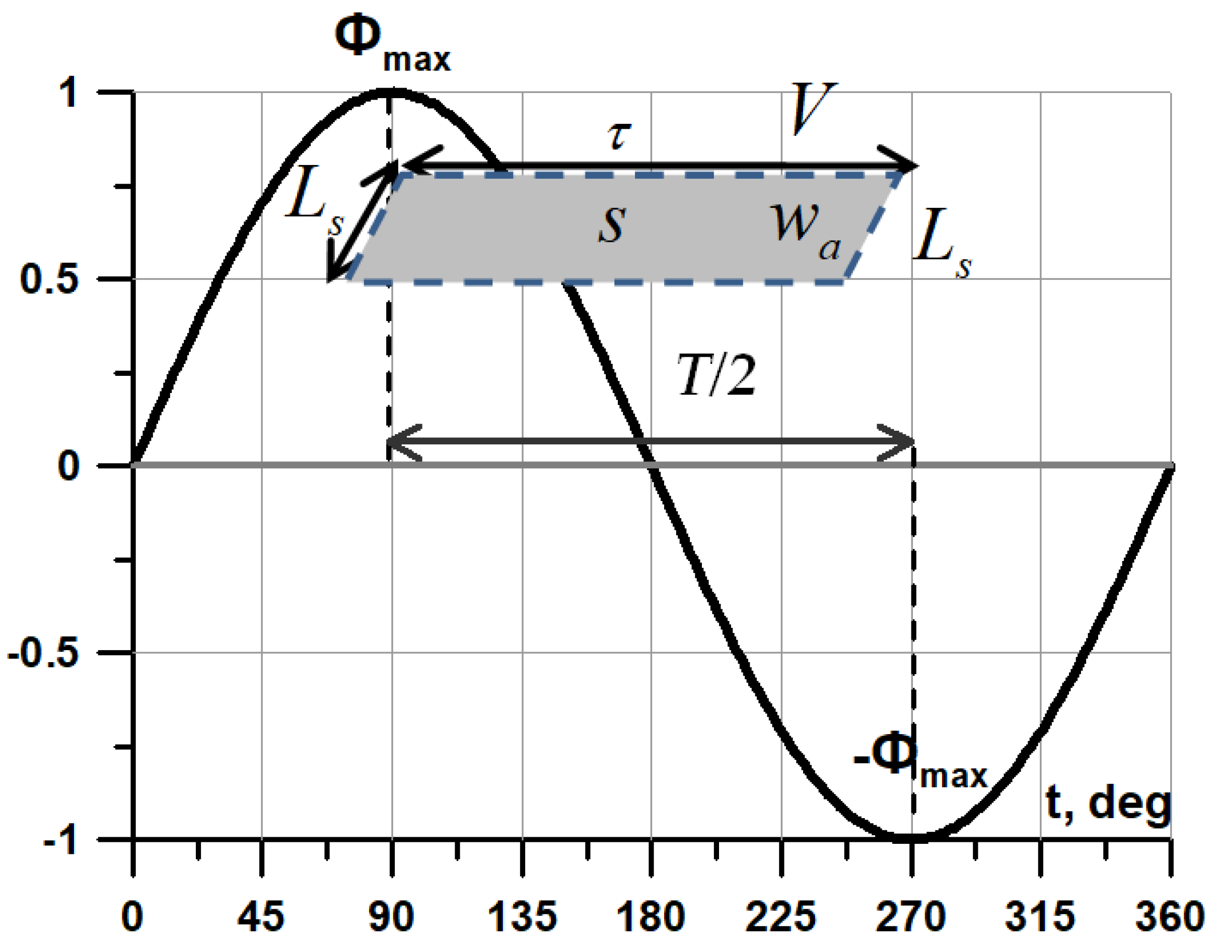
The basic physical law underlying the operation of any rotating-type electrical machine is Faraday’s law. An example of the physical meaning of the law is shown in Figure 1. On the horizontal axis, the time is conventionally plotted (measured in electrical degrees) through one change period T of excitation magnetic flux coupled to AW frame.

A rectangular armature winding coil with the number of turns $w_a$ moves at a speed $V$ relative to the sign-alternating sinusoidal magnetic field ${\Phi }_{\max }$ with an inductor flux amplitude (see Figure 1). The side of the coil perpendicular to the velocity vector is called the active length $L_s$ of the conductor, and the side parallel to the velocity vector is equal to the distance $\tau$ between the inductor’s adjacent poles. According to Faraday’s law, when flux leakage $\Psi$ with the coil changes, an EMF with an average value $E_{mean}$ is induced in it.

Flux leakage is the product of flux through the coil and the number of turns in it:

$$\Psi =\Phi \cdot w_a.$$

(11)

Then, the law can be expressed as follows:

$$E_{mean}=-\frac{\partial \Psi }{\partial t}=-\frac{\partial \Phi }{\partial t}\cdot w_a=-\frac{\Phi -(-\Phi )}{\partial t}\cdot w_a=-\frac{2\cdot \Phi }{T/2}\cdot w_a=-4\cdot \Phi \cdot \frac{1}{T}\cdot w_a=-4\cdot \Phi \cdot f\cdot w_a$$

(12)

In time equal to half the period $\raisebox{1ex}{$T$}\!\left/ \!\raisebox{-1ex}{$2$}\right.$, the alternating flow changes in magnitude twice; therefore, a factor of 4 appears in the numerator. The reciprocal of the period can be replaced by the frequency of the change in the flow:

$$f=\frac{1}{T}.$$

(13)

The effective (RMS) value of EMF

$$E_0=-4\cdot k_f\cdot \Phi \cdot f\cdot w_a\cdot k_o$$

(14)

Can be obtained by multiplying the average value by form factor, for a sinusoid equal to:

$$k_f=\frac{\pi }{2\cdot \sqrt{2}}\approx 1.11,$$

(15)

where $k_o=k_p\cdot k_y\cdot k_c$ is armature winding coefficient consisting of products of distribution coefficients $k_p$, shortening $k_y$ and skewing $k_c$. $k_y=\sin \left(\frac{{\beta }_s\cdot \pi }{2}\right)$ denotes the shortening factor, and ${\beta }_s$ represents the relative step of armature winding shortening. The winding coefficient $k_o$ shows how many times the distance between the coil’s active sides differs in the direction of decreasing (or increasing) from interpole distance $\tau$.

The second important traditional assumption is the one of a sinusoidal distribution of the induced EMF. This allows, by differentiating the distribution of induction in the gap, one to obtain a cosine form of EMF distribution in time, lagging behind the sinusoidal flux by 90 electrical degrees. After obtaining the machine’s geometry design sketch and FEM simulation of magnetic fields, the armature winding coefficient can be clarified. Additionally, we can use the obtained redefined value $k_f$ for subsequent analytical calculations in the future.

At present, the use of the average value of induction $B_{\delta }$ instead of amplitude value of the first harmonic induction is due to the widespread use of FEM calculation programs where the calculation of exact values of flux $\Phi$ through the loop in the gap, the integral (average) value of induction $B_{\delta }$, its distribution function at the gap along $\tau$ and the coefficient of its shape $k_f$ presents no difficulty. The traditional amplitude value of the first harmonic induction can be expressed in terms of the average.

$$B_{\max }=k_f\cdot k_a\cdot B_{\delta }\approx \frac{\pi }{2\cdot \sqrt{2}}\cdot \sqrt{2}\cdot B_{\delta }\approx \frac{\pi }{2}\cdot B_{\delta }.$$

(16)

The area of the gap is the product of pole overlap arc

$$\tau =\frac{\pi \cdot D_a}{2\cdot p}$$

(17)

and active armature length $L_s$:

$$s=\tau \cdot L_s.$$

(18)

Moreover, the relative circumferential speed of stator with AW can be expressed as the product of the circumference of armature bore $D_a$ diameter and the mechanical frequency of rotor n rotation.

$$V=\pi \cdot D_a\cdot \raisebox{1ex}{$n$}\!\left/ \!\raisebox{-1ex}{$60$}\right.,$$

(19)

We can represent the calculation of the effective EMF value, omitting the “minus” sign, as follows:

$$E_0=k_f\cdot B_{\delta }\cdot L_s\cdot \left(\pi \cdot D_a\cdot \raisebox{1ex}{$n$}\!\left/ \!\raisebox{-1ex}{$60$}\right.\right)\cdot 2w_a\cdot k_o.$$

(20)

It is clear that the last formulation of Faraday’s law is equivalent to the formulation of EMF occurrence in a conductor of length $L_s$ moving at a speed $V$ in a perpendicular magnetic field $B_{\delta }$. The difference is the availability of two conductors with an active length $L_s$, which are the sides of turns $w_a$ of one armature coil, connected in series, each of which moves in the same direction, but in the field of the opposite local direction. That is why there is a factor of 2 in the equation.

Characteristic values of the maximum induction $B_{\delta }$ are determined by the saturation induction of the ferromagnetic core of the yoke of both the stator and rotor, teeth, the relative teeth width, the value of working non-magnetic gap $\delta$ and the value of MMF of excitation field winding. A number of FEM calculations showed the possibility to achieve values of average induction in the gap of inductor machine with combined superconducting excitation up to 1.1–1.2 T. A further increase in the induction value in the gap of iron machine leads to an unjustified increase in yoke thickness and weight of the machine in order to prevent oversaturation.

2.4. The Main Calculation Equation of Electric Machines

The main calculation equation, also previously known as Arnold’s formula, allows one to switch from the nominal electrical parameters of a rotating electric machine to its geometric dimensions. The main dimension of rotary type machine is the armature bore diameter $D_a$. The second key dimension is the active axial length of armature $L_s$.

Entering the coefficient of the relative length of armature $\lambda =\frac{L_s}{D_a}$, it is possible to substitute the variables later on and take the axial length $L_s$ from the equation.

Input power, for the generator, which is the mechanical power applied to its shaft.

$$P_1=M\cdot \Omega ,$$

(21)

where $M$ is the rated mechanical torque, which is converted into electrical power.

$$S=m\cdot U\cdot I_a.$$

(22)

The output apparent power $S$ of the electrical generator is related to active power $P$ (also called electromagnetic power), according to vector diagram, through the power factor $\cos \phi$. The total output power (apparent power) $S$ and reactive power $Q$ of the machine are defined, respectively, as follows:

$$S=\frac{P}{\cos \phi }=\sqrt{P^2+Q^2},$$

(23)

$$Q=S\cdot \sin \phi ,$$

(24)

The reactive power present due to the inductance of load connected to the generator does not perform any useful work. However, the circulation of reactive current through the AW leads to additional electrical losses and wire heating. The output useful active electrical power (true power) of all phases of the generator is calculated as follows:

$$P_2=m\cdot U\cdot I_a\cdot \cos (\phi )\cdot \eta ,$$

(25)

where $\eta$ denotes machine efficiency, $m$ denotes the number of phases, which is usually three, $\cos \phi$ denotes the power factor specified by the task, showing the ratio of the active load power to the apparent one. For generators operating on a rectifier load, $m$ = 6 in order to reduce the amplitude of the output voltage ripples. Traditionally, the efficiency factor $\eta$ was not included in the formula for calculating the output power of a machine working in the network. However, if electric generators are used as part of electric propulsion systems (EPS), where floating frequency direct drive generators operate on their own rectifiers, the generator’s output net power is the input specified power of the rectifier. Additionally, when calculating the EPS, the parameters of nominal power of all the converter devices included in the system must be set starting from the nominal power of its final power element—the mover’s useful power.

We can shift from the rated voltage at load $U_L$ to EMF $E_0$ through the cosine of demagnetization angle $\psi$, between EMF and the current, as follows:

$$\psi =\left|\phi +\theta \right|,$$

(26)

$$P_2=m\cdot E_0\cdot \cos (\left|\phi +\theta \right|)\cdot I_a\cdot \eta ,$$

(27)

where $\phi$ denotes the reactive power angle, between the active voltage drop across the load $U_L$ (collinear to phase current $I_a$) and generator phase voltage $U$, $\theta$ denotes the load angle, between phase voltage $U$ and EMF $E_0$, also known as rotor angle.

Modulo values are indicated to take into account the direction of angles for the motor mode.

Expanding EMF (20) (given in square brackets), you can denote the useful output power (27) of the generator in the following form:

$$P_2=m\cdot \left[k_f\cdot B_{\delta }\cdot L_s\cdot \left(\pi \cdot D_a\cdot \raisebox{1ex}{$n$}\!\left/ \!\raisebox{-1ex}{$60$}\right.\right)\cdot 2w_a\cdot k_o\right]\cdot I_a\cdot \eta \cdot \cos (\left|\phi +\theta \right|).$$

(28)

It is clear from the formula that the power of an electric machine depends linearly on the density of magnetic flux (induction) $B_{\delta }$ in the working gap. However, for iron machines $B_{\delta }$, it is limited by teeth saturation induction $B_z$. If tooth thickness is approximately equal to the width of the slot, $B_{\delta }\approx 0.5\cdot B_z$.

We can increase the induction in the gap by thickening the tooth on account of narrowing the slot. In this case, the area of the slot is determined by the constructive current density in AW. For electrical machines with a resistive AW, the design current density is determined by the stacking density of the turns (the fill factor of the slot with copper) and thermal balance between cooling system intensity and heat generation in AW turns with a small wire cross-sectional area. A decrease in current density due to an increase in the groove area deeper down leads to an increase in the external overall size of the machine and leakage fluxes. The use of a superconducting AW with a high nominal current density makes it possible to significantly reduce slot width, in spite of additional thickness of individual cryostats, without increasing its depth. This makes it possible to thicken the teeth and increase the nominal induction in the working gap without causing oversaturation.

Linear load $A$ is a specific parameter characterizing the total current in the armature winding of an electric machine, distributed along the circumference of armature bore diameter $D_a$:

$$A=\frac{m\cdot I_a\cdot 2w_a}{\pi \cdot D_a}.$$

(29)

For traditional electrical machines with resistive windings, the cooling conditions are determined by intensity: 20,000–25,000 A/m—self-ventilation; 25,000–30,000 A/m—blowing; 30,000–35,000 A/m—channel oil; 70,000–75,000 A/m—jet evaporation [32]. For superconducting windings, the linear load is determined by the tape current-carrying capacity, which depends on coolant temperature and the efficiency of its supply to the central turns of HTS (high-temperature superconductor) armature windings, material and thickness of substrates and stabilizing layers of HTS tape, the magnitude of AC losses, which depend on frequency, as well as on the magnitude of the external magnetic field. The maximum permissible values of a linear load of fully superconducting electrical machines have not yet been experimentally confirmed. According to preliminary estimates, they may be in the 80,000–400,000 A/m range. A further increase in the linear load leads to a significant increase in slot depth, leakage fluxes and (despite the reduced stator bore) increase in the machine’s outer diameter. It also worsens the conditions for cryogenic cooling of central turns of armature windings, which release heat due to operation on alternating current. An excessive increase in the linear load can be rational for high-speed electrical machines that have strength limitations in regard to the rotor’s circumferential speed and diameter. We should also keep in mind the demagnetizing effect of armature reaction field on permanent magnets that may be a part of the inductor. To reduce the size of active zone, it is necessary to simultaneously increase the nominal induction value $B_{\delta }$ in the working gap and nominal current load $A$. An increase in induction can be achieved through the joint use of superconducting windings of axial excitation and high-coercivity permanent magnets on the rotor, which are protected from demagnetization by shunting axial flow ferromagnetic poles of the inductors of adjacent packages of the machine with combined excitation [33]. Linear load can be increased by using a superconducting armature winding cooled by liquid nitrogen at normal pressure to a temperature of 77 K and lower (down to 65 K) using supercooled nitrogen or liquid hydrogen [34].

Replacing the variables associated with armature current and linear load (29), we can obtain the following expression to calculate the power:

$$P_2=A\cdot k_f\cdot B_{\delta }\cdot \lambda \cdot {\pi }^2\cdot D_a{}^3\cdot \raisebox{1ex}{$n$}\!\left/ \!\raisebox{-1ex}{$60$}\right.\cdot k_o\cdot \eta \cdot \cos (\left|\phi +\theta \right|)$$

(30)

By delivering armature bore diameter $D_a$ from here, we will obtain the main calculation equation [3], as follows:

$$D_a=\sqrt[3]{\frac{P_2}{{\pi }^2\cdot k_f\cdot k_o\cdot A\cdot B_{\delta }\cdot \lambda \cdot \raisebox{1ex}{$n$}\!\left/ \!\raisebox{-1ex}{$60$}\right.\cdot \cos (\left|\phi +\theta \right|)\cdot \eta }}$$

(31)

It can be seen from the main calculation equation that an increase in the internal parameter values of the machine $A$ and $B_{\delta }$ (in denominator) affects the decrease in bore diameter. High values of nominal load angle $\theta$ can reduce the power factor $\cos \phi$ to zero (short circuit mode), which implies the need to increase the nominal EMF by automatically resizing the armature bore diameter $D_a$ in order to maintain the nominal generator voltage $U$, compensating for the active voltage drop on load $U_L$. The option of significant compensation by oversizing MMF of the inductor can lead to local oversaturation of the magnetic circuit. In addition, MMF of an inductor with a resistive FW is limited by the presence of free space between the poles and heat generation due to losses in active resistance. MMF of permanent magnet inductor is limited by the strength of retaining bandage. If compensation is not provided by including the nominal load angle $\theta$ in the main calculation equation, a decrease in phase voltage $U$ below the nominal voltage becomes inevitable. An increase in the relative length $\lambda$ by more than 3, without the use of intermediate bearings and a thick rigid shaft, will reduce the rotor’s natural frequency and can lead to mechanical resonance when rated speed is reached. The remaining parameters are fixed by the task and are not variable.

Some variables from the denominator can be combined into the so-called use factor [35] measured in magnetic pressure units Pa:

$${\sigma }_{}=\raisebox{1ex}{${\pi }^2$}\!\left/ \!\raisebox{-1ex}{$60$}\right.\cdot k_f\cdot k_o\cdot A\cdot B_{\delta }.$$

(32)

The Esson coefficient is sometimes used to evaluate the specific volumetric moment of low-speed machines, which is also measured in magnetic pressure units usually expressed in the following format: $\frac{kW\cdot \min }{m^3}$

$$C_e=\frac{2\cdot \pi \cdot M}{D_a{}^2\cdot L_s}.$$

(33)

2.5. The Principle of Operation of a Synchronous Generator, Illustrated by Phasor Diagram

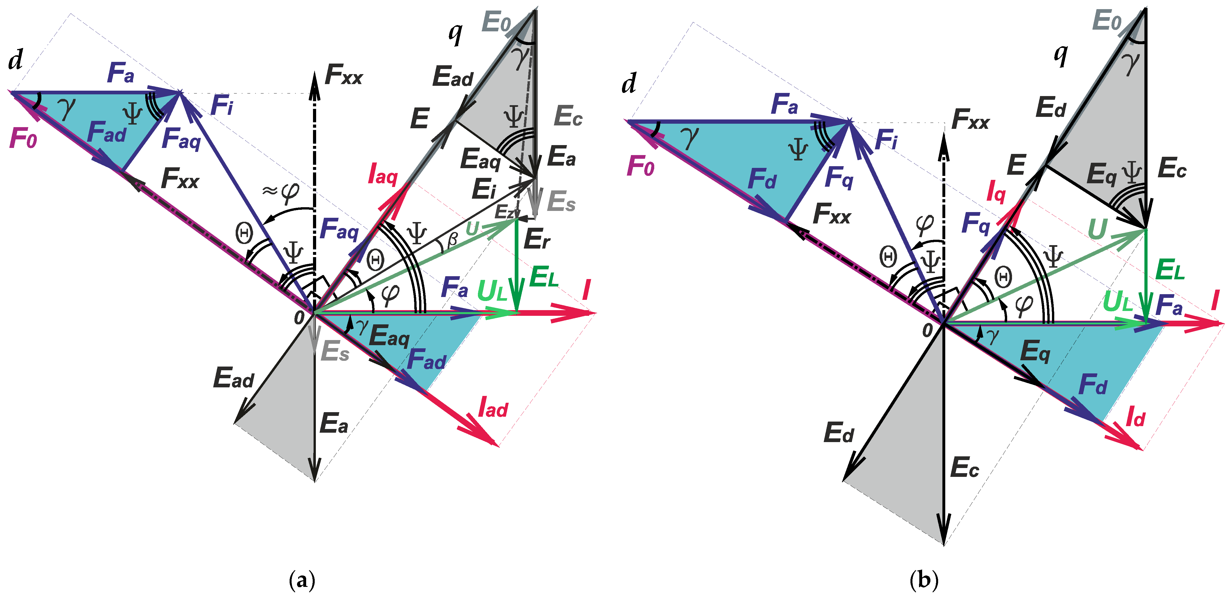
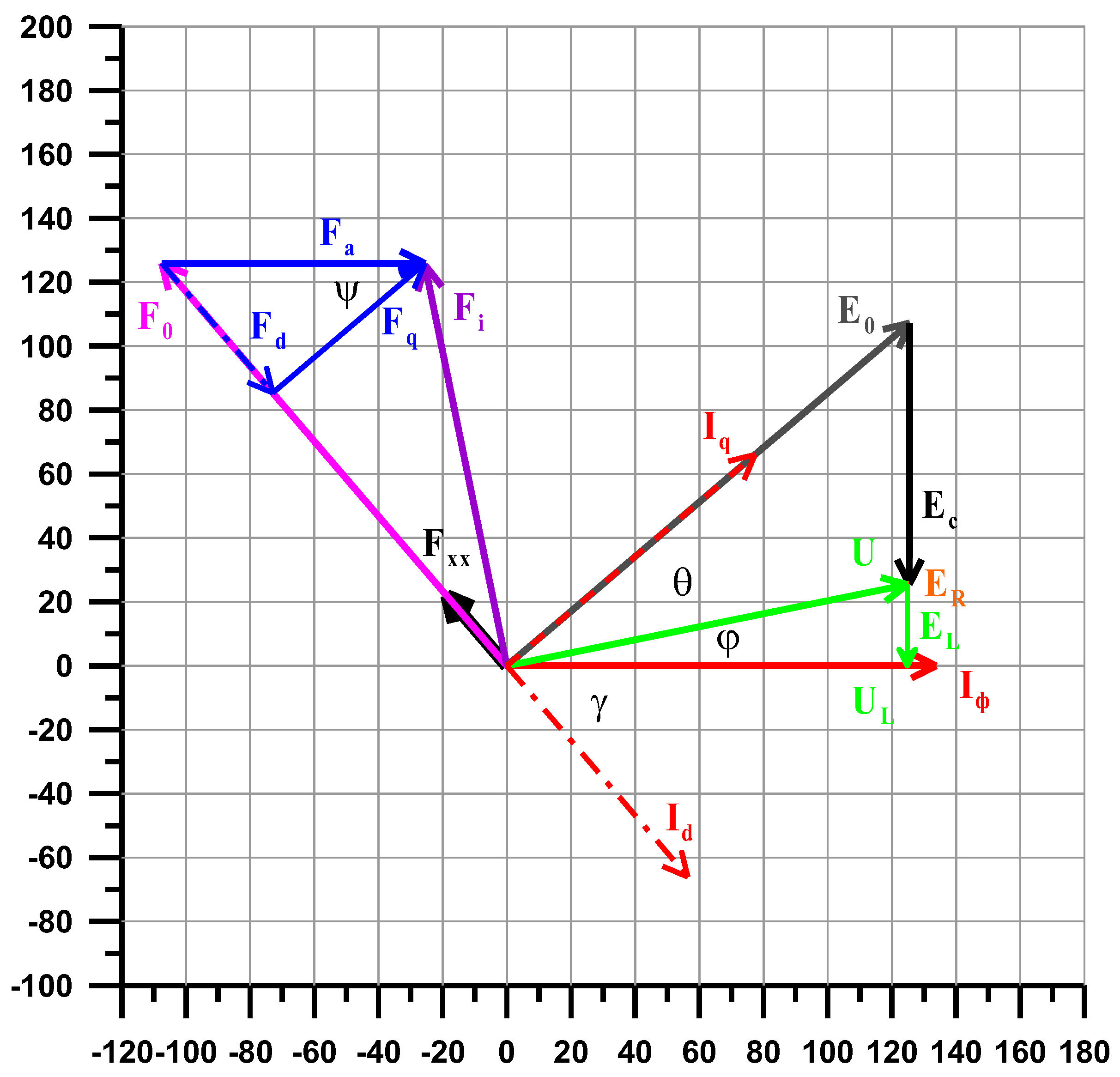
Diagrams are shown in Figure 2a,b. It is easy to see that the MMF triangles and EMF triangles are similar (shown in cyan and gray). Currents, which are multipliers of the corresponding MMF, and generating magnetic fluxes have no time shift—they are collinear and proportional.

• d—longitudinal axis of the electrical machine passing radially in the middle of the inductor pole;
• q—transverse axis of the electrical machine passing radially between the inductor's poles;
• $I$—phase current in the armature winding flowing through the load (for generator mode) or power source (for motor mode);
• $I_d$ and $I_q$—longitudinal and transverse currents, components of armature current projection on longitudinal d and transverse q axes;
• $F_a$—MMF of armature winding;
• $F_d$ and $F_q$—projection components of MMF of AW on the longitudinal d and transverse q axes;
• $F_{xx}$—MMF FW for no-load mode;
• $F_0$—the total MMF of the inductor necessary to induce the required EMF $E_0$ in AW;
• $F_i$—geometric sum of MMF of inductor and armature;
• $U$—voltage between phases, for the motor mode, equal to the mains voltage;
• $U_L$—rated active voltage, which is a multiplier of active power;
• $E_0$—total EMF in AW phase, necessary to maintain the nominal value of phase voltage;
• $E$—EMF in AW phase for no-load mode;
• $E_a$—EMF of armature reaction self-induction, inductive voltage drop in AW;
• $E_d$ and $E_{ad}$—components of EMF projection of the armature self-induction reaction on the transverse axis q, with and without allowance for leakage fluxes;
• $E_q$ and $E_{aq}$—components of EMF projection of the armature self-induction reaction on the longitudinal axis d, with and without allowance for leakage fluxes;
• $E_s$—EMF of AW leakage flux;
• $E_i$—EMF generated by the geometric sum of magnetic fields of the inductor and AW;
• $E_c$—the total synchronous inductive resistance of AW, including the sum $E_a$+$E_s$;
• $E_r$—voltage drop across the active resistance of AW;
• $E_L$—voltage drop on load reactance (for generator mode) or additional motor reactance (for motor mode);
• $E_z$—the total resistance (impedance) of AW phase;
• $\phi$—load reactive power angle in generator mode, or reactive power of electric machine in motor mode: angle between current $I$ and voltage $U$;
• $\theta$—load angle: between voltage $U$ of a phase and EMF $E_0$;
• $\psi$—demagnetization angle: between current $I$ and EMF AW $E_0$, equal to the angle between MMF at no load and at rated load;
• $\gamma$—armature reaction angle, between the longitudinal axis of the pole of inductor d and MMF $F_a$ of the armature winding;
• $\beta$—leakage flux angle, between the phase voltage $U$ and EMF $E_i$—the sum of magnetic fields of the inductor and AW.

In the generator mode, the rotor of electric machine is driven with a frequency $n$ from an external drive. A DC excitation current $I_i$ is supplied to the excitation winding with the number of turns $w_i$, with the possibility of automatic regulation. Under the action of excitation, the magnetomotive force $F_{xx}$ (directed upwards in the diagrams) overcomes the magnetic resistance $R_m$, with an excitation magnetic flux arising collinear to the current $I_i$ and MMF of excitation $F_{xx}$, coupled to phase armature windings, and inducing in them, according to Faraday’s law, the no-load EMF lagging behind (collinear between themselves) excitation current, excitation MMF and excitation flux $\Phi$ at 90 electrical degrees (for no-load mode, directed to the right at the diagram).

Since the longitudinal d and transverse q axes of the machine are right-angled and any EMF always lags behind the inducing flow by 90 electrical degrees, the vast majority of triangles in the diagrams are rectangular. When considering the Behn-Eshenburg diagram, where a small triangle with legs of voltage drop on the inductive leakage resistance and on active losses is neglected, all triangles are right-angled (see Figure 2b).

Right-angled triangles can be built up to a rectangle (shown with dotted lines) with the diagonal corresponding to the hypotenuse. Since the opposite sides of the rectangle are equal, it is easy to carry out parallel shifts of vectors and triangles graphically along the diagram.

The longitudinal axis d, passing radially along the middle of the inductor’s physical pole, is collinear with the excitation flux $\Phi$, excitation MMF $F_0$ and excitation current $I_i$. The transverse axis q, passing radially between the inductor’s physical poles, is collinear to EMF $E_0$ induced by excitation flow $\Phi$ in AW.

It is possible to make projections on d and q axes of all values not collinear with the axes in order to obtain their components. The peculiarities of indices of EMF components of armature reaction self-induction $E_{ad}$ and $E_{aq}$ is that the component $E_{ad}$ induced by the longitudinal component $F_{ad}$ of MMF of the armature reaction lags behind by 90 degrees and is projected onto the transverse axis q. Additionally, $E_{aq}$ is taken from $F_{aq}$ onto the longitudinal axis d. When plotting diagrams, this angular lag is denominated using the multiplier [31]:

$$-j=e^{-j\frac{\pi }{2}}.$$

(34)

When active load ($\phi =0°$) with high resistance R_L is connected to armature winding phase terminals, a low current I begins to flow through AW and through the load. The voltage drops in this case.

$$U_L=R_L\cdot I,$$

(35)

The equation above is balanced by voltage $U$ at generator terminals and is equal in magnitude to the induced EMF $E_{xx}$. When the load resistance decreases to nominal value, the current increases to its nominal value. An increase in the current flowing through AW leads to a proportional increase in MMF of armature $F_a$, generating an armature reaction flux directed in the diagram collinear to the current I of the phase. The alternating magnetic flux flowing through AW leads to EMF self-induction $E_a$ in AW, directed downward. Load angles $\theta$ and, accordingly, the total demagnetization angle $\psi$ increase. A part of magnetic flux from current flow in AW is closed without coupling with the excitation winding (leakage fluxes), and does not have any mutual effect on the excitation flux. However, it also induces scattering self-inductance EMF $E_s$ in AW, similarly to $E_a$, directed downwards in the diagram. The sum of total self-induction EMFs is called the synchronous inductive voltage drop in AW, as follows:

$$E_c=E_a+E_s$$

(36)

The corresponding inductive reactances can be expressed as follows:

$$X=\frac{E}{I}=2\cdot \pi \cdot f\cdot L,$$

(37)

where inductive reactances $X$ are related to the inductance of winding $L$ and frequency of flux change $f$.

Components of total inductive resistances of the projections on longitudinal d and transverse q axes, taking into account the inductive scattering resistance $X_s$, can be expressed as follows:

$$X_d=X_{ad}+X_s,$$

(38)

$$X_q=X_{aq}+X_s,$$

(39)

$$X_a=\sqrt{X_{ad}+X_{aq}},$$

(40)

$$X_c=\sqrt{X_d+X_q}.$$

(41)

The sum of all electric machine losses released in the form of heat, consisting mainly of resistive losses in AW for traditional machines with intensive cooling, is the active power, which can be represented at a first approximation in the form of a voltage drop across the active resistance directed opposite to the current. Since for an optimally designed machine, the amount of losses in the windings is approximately equal to the amount of losses in the ferromagnetic cores (electrical losses are equal to magnetic losses), then the total active voltage drop can be considered to be twice the electrical losses.

$$E_r=\frac{S\cdot \cos \phi \cdot \left(1-\eta \right)}{m\cdot I}~2\cdot R_a\cdot I,$$

(42)

The minor reactive rotation of vector $E_r$, due to the low inductance of Foucault eddy currents in thin sheets of laminated armature magnetic circuit, can be neglected. For electric machines with a superconducting AW, the active resistance $R_a$ is much less than that in the case of resistive winding; however, it is not equal to zero due to the presence of active losses in alternating current superconductors. One of the advantages of superconducting windings is a reduction in ohmic losses in AW, and a reduction almost to zero of the length of voltage drop vector across the active resistance. It can be seen from the formula that when efficiency $\eta$ increases through the use of superconducting windings and thin-sheet siliceous electrical steel, the already small length of vector $E_r$ tends toward zero. Insignificant losses make it possible to increase the magnitude of linear load $A$, for resistive windings, limited solely by cooling system efficiency. According to the main calculation equation, this will make it possible to asymptotically reduce the size of the active zone.

The MMF value of armature winding can be denoted as follows:

$$F_a=\frac{m\cdot k_a\cdot I_a\cdot 2w_a\cdot k_o}{\pi \cdot 2p},$$

(43)

where $k_a$ is the amplitude coefficient, equal to $\sqrt{2}$ for a sinusoid, and it can be represented as directly proportional to the linear load, as follows:

$$F_a=A\cdot \frac{k_o}{2\cdot k_f}\cdot \frac{\pi \cdot D_a}{2p}=\frac{A\cdot \tau \cdot k_o}{2\cdot k_f},$$

(44)

Thus, the rise in the nominal linear load $A$ increases the armature reaction flux and the magnitude of voltage drop in the synchronous inductive reactance $E_c$ almost proportionally. If the source of MMF excitation of a machine with a superconducting AW is a resistive FW, or permanent magnets, it will be impossible to fully compensate for the synchronous voltage drop in the superconducting armature winding, and the generator’s load characteristic U(I) will go down sharply. In addition, the high armature reaction flux of a superconducting FW with a high linear load can critically demagnetize even high-coercivity permanent magnets. A decrease in the generator output voltage below the nominal voltage with an increase in the load current has a significant negative impact on consumer devices connected as load. For example, within the EPS, a decrease in voltage will lead to a change in the operation mode of the propulsion unit. The rectifier can be a controlled one to compensate for the voltage level of EPS power generator. However, this significantly complicates the rectifier itself. Therefore, the task of maintaining a constant level of a synchronous generator’s output voltage, regardless of the magnitude of the current load, remains relevant.

With an increase in the load that has an inductive component ($\phi >0°$), the voltage at generator terminals $U$ differs $\cos \phi$ times from the active load voltage $U_L$. Cathetus $E_L$ in the opposite corner $\phi$ is the voltage drop across the inductive resistance of the load. The generator spends reactive power to overcome it. To maintain the nominal value of voltages $U$ and $U_L$, it is necessary to resize the machine in order to increase $E_0$. From voltage diagram and the main calculation equation, which provides compensation for the inductive load voltage drop, we can see that a generator operating on a resistive load ($\phi =0°\to \cos \phi =1$) or directly on rectifier will have an active zone smaller than that of a generator working for a power line network with the possibility of connecting an inductive load to it.

When the generator is operating on a load that has a capacitive component, the load angle becomes negative $\phi <0°$ and the voltage lags behind the current. In such a case, the generator may have a relatively reduced armature bore diameter $D_a$.

With an increase in the load current $I$, which also flows through AW $I=I_a$, MMF of armature $F_a$ and the flux of armature reaction and voltage drop $I\cdot X_c$ across the synchronous inductive resistance $X_c$ increase, which can also be represented as EMF of AW self-induction $E_c$. If EMF $E_0$ induced in AW in the process of increasing the load current $I$ is not increased by raising MMF excitation $F_{xx}$ by value $F_{ad}$, the projection of the end of vector $E_0$ on the current axis $I$ will show an uncompensated decrease in voltage level $U_L$ on the load. Traditionally, for generator mode, to compensate for a voltage drop due to armature reaction, the overexcitation factor is set as follows:

$$\epsilon =\frac{E_0}{U}=\frac{\cos \phi }{\cos \psi }\approx [1.05,1.75].$$

(45)

For superconducting machines with high linear load and armature reaction MMF, the overexcitation factor $\epsilon$ can be set at over 1.66.

The main difference between the Blondel diagram and the Potier diagram is that the Blondel diagram is built for a salient-pole machine, with inductive reactances of different magnitudes $X_d\ne X_q$. With the Blondel diagram, formally, the hypotenuse $E_a$ of a right triangle $E_{ad}$$E_{aq}$$E_a$ is not strictly perpendicular to the current axis $I$. However, for practical implementation of a significant magnetic anisotropy of the electric machine’s inductor, it is necessary to use in the design [36] special diamagnetic elements made of bulk HTS ceramics cooled to temperatures significantly below the boiling point of liquid nitrogen. Therefore, for all other machines, to start the calculation, one can make an assumption about an insignificant explicit polarity, perpendicularity of vector $E_a$ to the current $I$, as in the Potier diagram for an implicit-pole machine, and in the simplified Behn-Eshenburg diagram.

The calculation of the required excitation MMF $F_{xx}$ for no-load mode, when there is no AW current and armature reaction field, is carried out according to Ohm’s law for magnetic circuit. The total MMF of armature reaction $F_a$ is easily calculated from the linear load $A$ of the armature. It is necessary to use the diagrams to calculate the value of MMF $F_{ad}$ of the longitudinal component of armature reaction field. It can be seen from the diagram that projection $F_a$ onto the longitudinal axis d is calculated as follows:

$$F_{ad}=F_a\cdot \cos \gamma ,$$

(46)

where angle $\gamma$ is armature reaction angle between the field of the inductor pole and armature current field, as follows:

$$\gamma =90°-\psi =\frac{\pi }{2}-\left(\phi +\theta \right).$$

(47)

Thus, calculation of value $E_0$ is necessary for compensation of voltage drop $U_L$ across the load, due to armature reaction, for nominal angle $\psi$. Excitation MMF is calculated as follows [17,35]:

$$F_0=F_{xx}+F_{ad},$$

(48)

where $F_{xx}$ is the total drop in magnetic potential $U_m$ in sections of the magnetic circuit calculated using the equivalent circuit method for the magnetic circuit according to the laws of Ohm and Kirchhoff.

It is easy to see from the diagram that a direct increase in the magnitude of the excitation MMF $F_0$ leads to a multiple increase in all EMF of AW. In addition to the positive effect, in the form of an increase in EMF $E_0$ of AW, self-induction EMF $E_a$ also increases by multiple times, reducing the generator’s output voltage $U$.

2.6. Calculation of AW Synchronous Inductive Reactance

The traditional analytical calculation of parameter $X_c$, which has the strongest influence on the output voltage of generator $U$ and includes the empirical coefficients of bringing MMF of armature reaction to MMF of excitation winding $k_{\delta }~1,$$k_{\mu }~2$, is suitable only for iron machines with a classic tooth-slot zone of armature magnetic circuit and poles of a traditional shape. Additionally, the main disadvantage is the lack of consideration for the magnetic state of magnetic cores $\mu$ in the nominal mode. Therefore, the actual value $X_c$ may differ from the calculated one in multiples. Direct experimental $X_c$ measurement with the use of an RLC-meter, on alternating current with a fixed rotor, is associated with a significant error due to the shielding effect of metal structural elements on the path of the magnetic flux of armature reaction: iron cores (especially unlaminated ones), solid inductor yoke, pole pieces, shaft, bandage, the rotating cryostat, fastening hardware, dowels, permanent magnets, damper (starting) short-circuited rotor winding, etc.

The most reliable values of inductive resistances, taking into account the specified nonlinear magnetic properties of the applied magnetic circuits, are those obtained exclusively as a result of three-dimensional FEM computer simulation. However, such modeling can be carried out only after obtaining a detailed three-dimensional design sketch of the entire rotor and stator structures, including armature end-winding. Therefore, the task of a simple and universal preliminary analytical calculation of AW inductive resistances is especially relevant. Classical formulas [27,28,37] show only the qualitative influence of various parameters.

The synchronous impedance consists of the sum of AW inductive reactance $X_a$ and leakage AW inductive reactance $X_s$, as follows:

$$X_c=X_a+X_s$$

(49)

It can be seen that the inductive reactance $X_a$ of AW is as follows:

$$X_a=2\cdot m\cdot f\cdot \frac{{\mu }_0}{k_{\delta }\cdot k_{\mu }\cdot \delta }\cdot D_a\cdot L_s\cdot \frac{w_a{}^2\cdot k_o{}^2}{p^2}$$

(50)

In addition, it depends quadratically on the number of turns $w_a{}^2$ of AW; therefore, it is necessary to reduce the number of turns, but, while maintaining MMF of AW, proportionally increase the phase current, simultaneously increasing MMF of the inductor, so as not to reduce the generated EMF and the generator’s output voltage. However, an increase in current, according to Joule–Lenz law, leads to a quadratic increase in electrical losses, as follows:

$$P_{JL}=m\cdot I_a{}^2\cdot R_a,$$

(51)

where $R_a$ is the active resistance of AW phase.

Thus, the only possible way to reduce the size of the active zone is the use of a superconducting AW, in which active resistance and losses, arising from losses in HTS wire on alternating current, can be neglected.

The second componentcontributing to the total synchronous inductive reactance is the leakage inductive reactance, as follows:

$$X_s=8\cdot m\cdot f\cdot \pi \cdot {\mu }_0\cdot L_s\cdot w_a{}^2\cdot k_o{}^2\cdot \frac{\Sigma {\lambda }_m}{z_s},$$

(52)

where $z_s$ is the number of armature slots (teeth), $\Sigma {\lambda }_m$ is the sum of magnetic conductivities of slots, frontal and differential leakage. Accurate calculation of magnetic conductivities is one of the most time-consuming analytical tasks, taking into account the specific geometry of the entire active zone and frontal parts of the windings. However, for unsaturated iron machines, leakage fluxes are negligible and leakage inductive reactance can be neglected there. For iron-free superconducting machines, relatively small inductive resistances are comparable in magnitude. Armature reaction flux coupled to the FW (inductor) may be less than the leakage flux. In this case, the leakage inductance can be even greater: $X_s>X_a$. The pattern of magnetic flows in an ironless machine is three-dimensional and cannot be built in a flat approximation, which requires a three-dimensional FEM simulation to obtain accurate $X_c$ values. A separate calculation of the $X_s$ component via modeling is rather complicated, and requires the calculation of intrinsic and mutual inductances of FW and AW, taking into account the magnetic state of iron cores; however, it has no fundamental practical significance. The transition from Blondel diagram to Behn-Eshenburg or Rotert diagrams makes it possible, among other things, not to take the scattering resistance into account separately in formal terms.

The common disadvantages of iron-free superconducting electrical machines are the insufficient current-carrying capacity of HTS-2G tapes in the temperature range of boiling liquid nitrogen, and the critical decrease in current-carrying properties when the tapes are directly in the inductor’s magnetic field. Additionally, the absence of light and strong non-metallic isotropic structural materials (with the possibility of precision manufacturing, high rigidity and strength, low thermal expansion coefficient) that work stably at cryogenic temperatures is also considered a disadvantage.

The simplest way to make an initial estimate of the order of magnitude $X_c$, before calculating any dimensions, is to plot a vector diagram, where the nominal load angle $\theta$ is initially set to a value chosen from a narrow range of possible values based on previous designing experience. In this case, the calculation error $X_c$ is proportional to the ratio of sines of the given and real angles $\psi =\pm \phi \pm \theta$. It should also be kept in mind that the angle $\phi$ included in the angle $\psi$ as a component, is not a constant and changes in the process of variation of magnitude and type of the connected electrical load, which, to a sufficient extent, levels out the error in choosing the nominal value of angle $\theta$. Thus, the main task of designing an electric machine operating in the generator mode is fulfilled—ensuring that the nominal value of the output voltage is maintained, regardless of the current value and type of connected load, without significant resizing of armature bore diameter.

The choice of nominal value of angle $\theta$ is determined by the generator’s overload capacity, i.e., the ability to exceed the rated load current without a significant reduction in rated voltage—power overload. Most manufacturers of electrical machines, for advertising purposes, indicate, firstly, as rated power, a short-term overload power, limited in time due to a sharp increase in heat generation; and secondly, the power at which voltage is critically reduced. It is possible to provide the rated value of voltage during current overload either by forcing the excitation current or by resizing the machine’s active zone.

It can be seen from the Blondel diagram that resizing begins with an increase in $E_0$ growth rate, when the longitudinal components of EMF of armature reaction and current become greater than the transverse ones, the demagnetization angle $\psi$ becomes higher than 45 degrees, and the angle is less than 45 degrees.

If the nominal angle of the load’s reactive power $\phi$ is rigidly fixed in the task, the operating angle for starting the analytical calculation can be chosen as follows:

$$\theta =45°-\phi .$$

(53)

For the motor mode, the most important aspect is the angle $\gamma =90°$ when the slots with phase current are opposite the middle of inductor’s poles, and the ampere force acting on them is at the maximum. Maintaining this angle $\gamma =90°$ is an important task for a brushless DC motor control system.

For short circuit mode, when the angle $\psi$ approaches 90 degrees, the voltage drops to almost zero and the vector $E_0$ is directed almost upwards; thus, there is no way to increase the value $E_0$ to such an extent that its projection on the current axis $I$ would give the nominal value of voltage $U_L$ at the load ($E_0\cdot \cos (90°)=0$). However, for fully superconducting systems, in which reactivity angle is close to $\phi \to 90°$, high voltage values $U_L$ are not required anyway.

The main inductive resistance of armature winding phase of a non-salient pole ($X_d=X_q$) machine, or with a weakly pronounced difference between the longitudinal $X_d$ and transverse $X_q$ inductive resistances of the electric machine (with the ability to operate at a given power, both in motor mode and generator mode), taking into account voltage drop $E_c$ due to the presence of AW inductive resistance $X_c$, based on the condition of the continuity of vector diagram triangles, is unequivocally determined as follows:

$$X_c=\frac{\left|E_0\cdot \sin (\phi +\theta )-U\cdot \sin (\phi )\right|}{I_a}.$$

(54)

From the similarity of MMF and EMF triangles and proportionality of their initial and demagnetizing components, one can calculate the total excitation MMF as follows:

$$\frac{E_0}{E_c}=\frac{F_0}{F_a}\to F_0=\frac{E_0\cdot F_a}{E_c}=\frac{E_0\cdot F_a}{X_c\cdot I_a}.$$

(55)

If it is not possible to compensate for voltage drop during overcurrent by forcing the excitation current, for example, when using permanent magnets, or if there is no free space between the poles for a resistive FW on the rotor, or due to low efficiency of FW cooling system, or due to magnetic circuit oversaturation; then, it is possible to provide a resizing of the machine’s active zone in advance by increasing the nominal load angle and demagnetization. For example, an increase in the nominal demagnetization angle, in overload conditions, taking into account the multiplicity factor $k_I$ of current overload, is usually equal to 1.5 or 2.

$$\psi =a\tan \left[(\tan \left(\phi +\theta \right))\cdot k_I\right]$$

(56)

Thus, it corresponds to the following values:

$$a\tan \left[(\tan 45°)\cdot 1.5\right]\approx 56°,$$

$$a\tan \left[(\tan 45°)\cdot 2\right]\approx 63°.$$

The option of maintaining the nominal value of generator voltage during overload by only increasing the excitation current by $k_I$ times, in the case when overload compensation was not initially included in the core dimensions, will lead to a disproportionately small increment in excitation flux due to the saturation of steel in magnetic cores. This will lead to an asymmetric increase in magnetic induction $B_z$ in armature teeth, where the directions of magnetic fluxes of excitation $F_0$ and armature reaction $F_a$ coincide, as well as to a quadratic growth of magnetic losses in these zones. As a rule, the Potier diagram is shown next to the magnetization curve, where nonlinear correspondences of contribution of MMF excitation to excitation flux and armature winding EMF induced by it $\frac{F_0}{F_i}>\frac{E_0}{E_i}$ are plotted due to the nonlinearity of magnetization curve. However, the proportionality of coinciding and counter flow zones is determined by the value of demagnetization angle $\psi$. When the demagnetization angle is close to $\psi \to 90°$, MMF of excitation flows $F_0$ and armature reaction $F_a=F_{ad}$ become directed oppositely to each other $\gamma \to 0°$ and the cores are desaturated. For traditional machines with resistive windings, or permanent magnets, in which excitation MMF is limited, this mode is not a standard operating mode, since the total field in the gap has a strong dip in the middle, which leads to the induction of an EMF significantly different from the sinusoidal EMF in AW, and a deterioration in the quality of output voltage form. However, when working with a rectifier, the sinusoidal shape of generator’s output voltage does not play such a significant role. A superconducting FW with a high MMF is capable of overpowering the armature reaction field and correcting the critical dip in the field in the middle of the pole. Thus, in superconducting machines with ferromagnetic cores, where the current-carrying capacity of HTS tapes during deep cooling allows one to obtain a high MMF, the nominal operating angle $\theta \le 90°-\phi$ can be deliberately chosen relatively high in order to integrally reduce the magnetic losses.

2.7. Diagram Drawing Algorithm of a Synchronous Machine for the Mode of an Overexcited Salient-Pole Generator

The end of a vector is its tip with an arrow; the beginning of a vector is the opposite side without an arrow. Since the plotting order is from the logical result to the root cause, most of the vectors will be drawn from the end to the beginning.

The initial set parameters for the calculation are as follows:

• number of phases $m$;
• total electric power given delivered by generator $S$;
• rated phase voltage $U$;
• power factor $\cos \phi$;
• efficiency factor (not less than) $\eta$;
• the type of cooling system affecting the choice of the characteristic nominal value of linear load $A$.

The sought-after values are: EMF value $E_0$ induced in AW, which compensates for voltage drops due to the reaction of armature field and inductive/capacitive type of the load, and the required full MMF $F_0$ of FW excitation, providing a magnetic flux $\Phi$ sufficient for induction $E_0$, taking into account the demagnetizing effect of the armature reaction field.

According to the above formulas, we calculate and plot, on the selected scale, the following vectors.

• Rated phase current from (22) $I_a=\frac{S}{m\cdot U}$. We plot it from the center 0 of the diagram horizontally to the right with a right arrow;
• Active voltage drop across the load $U_L=U\cdot \cos \phi$. We plot it from the center of diagram 0 to the right, collinear to the current $I_a$;
• Load reactive power angle $\phi =a\cos (\cos \phi )$. When using computer programs to plot the diagram, the rated voltage of the generator can be plotted quite accurately by setting the value of the angle from the end of the horizontal vector $U_L$. However, for manual graphic-analytical drawing, the use of a protractor will not result in a good accuracy;
• Voltage drop across the load inductive reactance $E_L=U_L\cdot \tan \phi$ is the vertical opposite cathetus of angle $\phi$ of right triangle $U_L$0$U$. For active-inductive nature of the load, when angle $\phi$ is positive, it is plotted upwards from the end $U_L$, perpendicular to the current. For a capacitive load, when angle $\phi$ is negative, it is plotted with its beginning downwards;
• Let us draw the beginning from center 0 to the beginning $E_L$, with rated phase voltage $U$;
• The voltage drop due to active losses in the electrical machine is calculated (42) as $E_r=\frac{S\cdot \cos \phi \cdot \left(1-\eta \right)}{m\cdot I_a}$. It is relatively low. Formally, it can be plotted parallel to the current $I_a$, beginning to the right of the end of voltage $U$. For a superconducting machine with high efficiency, and to build simplified diagrams, it can be neglected;
• The operating angle $\theta$ can be calculated by taking into account the main parameters of the generator and the dimensions of armature active zone according to Formula (20) EMF $E_0$, where the values of the diameter $D_a$ from (31) are substituted, and the number of turns $w_a$, expressed from the selected linear load $A$ (29), are $w_a=\frac{\pi \cdot D_a\cdot A}{2\cdot m\cdot I_a}$;
• Neglecting, for an unsaturated iron machine, a separate voltage drop $E_s$ due to inductive leakage inductance resistance $X_s$, and assuming insignificant magnetic anisotropy of the salient-pole inductor ($X_d\approx X_q$), we plot, perpendicular to the current $I_a$, from the beginning of $E_r$ (or end of $U$), the vertical cathetus of the sum voltage drop on the inductive resistance of the phase of the armature winding and load $\left(E_c+E_L\right)$. It is formed by the projection of the end of the vector $E_0$ perpendicular to the horizontal axis of the current $I_a$ to the end of the vector $U_L$ and its length is calculated using the Pythagorean theorem: $\left(E_c+E_L\right)=\sqrt{E_0{}^2-U_L{}^2}$;
• The nominal demagnetization angle $\psi$ is calculated as follows:$\psi =a\tan \left(\frac{\left(E_c+E_L\right)}{U_L}\right)$. Usually, taking into account the provision of overcurrent, while maintaining the level of the rated voltage, the rated demagnetization angle is up to $\psi =\left(\phi +\theta \right)\le 56°$ for one and a half times overload, and $\psi =\left(\phi +\theta \right)\le 63°$ for double overload;
• At an angle $\psi$ to the basic horizontal axis of the current $I_a$, we draw an auxiliary transverse axis q, for rated load, on which we plot the vector $E_0$. Additionally, we can draw, passing through 0, the longitudinal axis d, perpendicular to the transverse axis q;
• The nominal load angle $\theta$ is calculated as (26) $\theta =\psi -\phi$. Usually, the nominal load angle is in the $\theta ~15°\mathrm{...35}°$ range. Large values of the nominal load angle lead to instability of the electric machine (especially in the motor mode) and the possibility of it falling out of synchronism with a sharp change in load. Small nominal operating angles lead to a significant oversizing of the diameter $D_a$;
• The total synchronous inductive voltage drop $E_c$ can be calculated as follows: $E_c=U_L\cdot \tan \psi -E_L$ The next urgent task is to calculate the required MMF of excitation $F_0$, taking into account the demagnetizing effect of the armature reaction field;
• According to Ohm’s law for magnetic circuit, based on the sum of magnetic potential $U_m$ drops in the sections, we can calculate the required no-load EMF $F_{xx}$, and plot it from 0 along the longitudinal axis d. For iron machines with unsaturated cores, with a non-magnetic gap $\delta$ of more than a few millimeters, which is typical for machines with a non-magnetic bandage or rotating cryostat, one can approximately calculate MMF of no-load mode excitation through the drop in magnetic potential only in the air gap (8) $F_{xx}\approx U_{\delta }$;
• From the linear load $A$ selected according to cooling conditions and designing experience, we can calculate MMF of armature reaction $F_a$ (44) and plot it from center 0 to the right in the direction of current $I_a$, collinear to it;
• Now, we draw perpendicular projections from the end of $F_a$, $F_{ad}$ (46) onto the longitudinal d and $F_{aq}$ onto the transverse q axes;
• Along the longitudinal axis d, we make a parallel transfer of the collinear axis of vector $F_{ad}$ from end to end to $F_{xx}$;
• Finally, we obtain the desired length of the total MMF excitation 0$F_0$, necessary to compensate for the demagnetizing effect of armature reaction and provide the rated voltage at load as the sum (48) $F_0=F_{xx}+F_{ad}$.

3. Results

As an example, according to the algorithm described above, a superconducting synchronous generator was calculated. The results are shown in

Table 2. Main parameters of an experimental prototype of a superconducting synchronous generator.

№	Parameter	Variable	Unit	Value
1	Number of phases	$m$	-	3 × 2
2	Total electric power given delivered by generator	$S$	kVA	102
3	Rated phase voltage	$U$	V	128
4	Power factor	$\cos \phi$	-	0.98
5	Efficiency factor	$\eta$	%	99.4
6	Linear load	$A$	A/m	200,000
7	Phase current	$I_a$	A	134
8	Active voltage drop across the load	$U_L$	V	125
9	Load reactive power angle	$\phi$	deg	11
10	Voltage drop across the load inductive reactance	$E_L$	V	25
11	Voltage drop due to active losses in the electrical machine	$E_r$	V	0.68
12	Nominal load angle	$\theta$	deg	29
13	Demagnetization angle	$\psi$	deg	40
14	Total synchronous inductive voltage drop	$E_c$	V	82
15	Electromotive forces of armature winding	$E_0$	V	165
16	Armature bore diameter	$D_a$	mm	134
17	No-load magnetomotive forces of excitation winding	$F_{xx}$	hAt	28
18	Magnetomotive forces of armature reaction	$F_a$	hAt	82
19	Magnetomotive forces of armature reaction projections to d axis	$F_d$	hAt	53
20	Total magnetomotive forces of excitation winding	$F_0$	hAt	165

and Figure 3.

As can be seen from the sum of the vectors $F_{xx}+F_d=F_0/2$, the prototype has a double margin for the MMF of the excitation winding.

4. Discussion

In traditional methods, a laborious calculation of all magnetic conductivities is necessary to calculate the synchronous inductive voltage drop. Such a calculation is intended for classical electric machines with a traditional tooth-slot zone, and contains many empirical formulas and non-physical coefficients. The accuracy of traditional calculations can only be verified by running an FEM simulation of the 3D problem. However, FEM simulations can be carried out only after obtaining the calculated geometry of the active zone with the exact dimensions of all elements. Incorrect results of magnetic conductivities’ calculation leads to insufficient excitation MMF and a critical decrease in the output voltage below the nominal value. In this case, the rated power value can be achieved for a short time only by overcurrent when forcing the excitation current. Additionally, when overexcited, the quality of the output voltage is critically reduced. If current overload is not foreseen at the beginning of calculation when determining the main dimensions of the active zone by including operating angles in the main calculation equation, current overload will lead to intense heat generation and emergency damage to winding insulation. Thus, the declared continuous rated power will not be achieved.

The algorithm for drawing phasor diagrams proposed by the author allows one to quickly perform an evaluative analytical calculation of the main parameters of the designed synchronous electrical machines, regardless of the active zone design: tooth-slot zone, types of windings and superconducting windings, with the accurate ratios of true and supposed angle sines of loads. The algorithm can be used to quickly assess the credibility of automated machine calculation results. The following conditions are used in the calculation:

• continuity of phasor diagram triangles;
• unsaturation of magnetic cores;
• high efficiency of the machine and insignificance of voltage drop on the active resistance of armature windings;
• insignificance of flux leakage;
• insignificance of the rotor’s magnetic anisotropy.

5. Conclusions

• Basic equations for calculating a synchronous electrical machine are presented in this work.
• Combined diagrams of MMF and EMF of salient-pole synchronous electric machines for the generator mode are plotted. The similarity between MMF and EMF triangles is demonstrated.
• The algorithm for constructing a diagram of a synchronous machine for the generator mode is proposed. The characteristic load angle (including the overcurrent mode) is reasonably chosen as the initial data, and the calculation of synchronous inductive resistance value can be the desired result of creating the diagram. This allows one to quickly obtain all the main parameters of the designed machines (including non-traditional ones) before calculating all the geometric dimensions of the structure.
• It is shown that an increase in the nominal value of linear load of a superconducting AW leads to a multiple increase in armature reaction MMF, and, as a result, to a critical voltage drop across the inductive resistance of armature winding. Voltage drop at generator terminals can be compensated for by the initial inclusion of the nominal demagnetization angle in the main calculation equation, and partially compensated for by an increase in excitation MMF only.
• The use of a superconducting AW with a high current-carrying capacity and constructive current density makes it possible to narrow the slots and expand the teeth, increasing the average induction in the working gap to 1.1 T.
• We have analyzed the option of increasing the specific power of a fully superconducting synchronous generator by means of a nominal operation mode at armature reaction angles close to 0 degrees (when FW and AW flows are opposite) in order to de-saturate the magnetic circuit of the ferromagnetic cores and reduce magnetic losses or the area of magnetic circuits.