
Chart Classification Using Siamese CNN


Abstract
:1. Introduction
2. Related Work
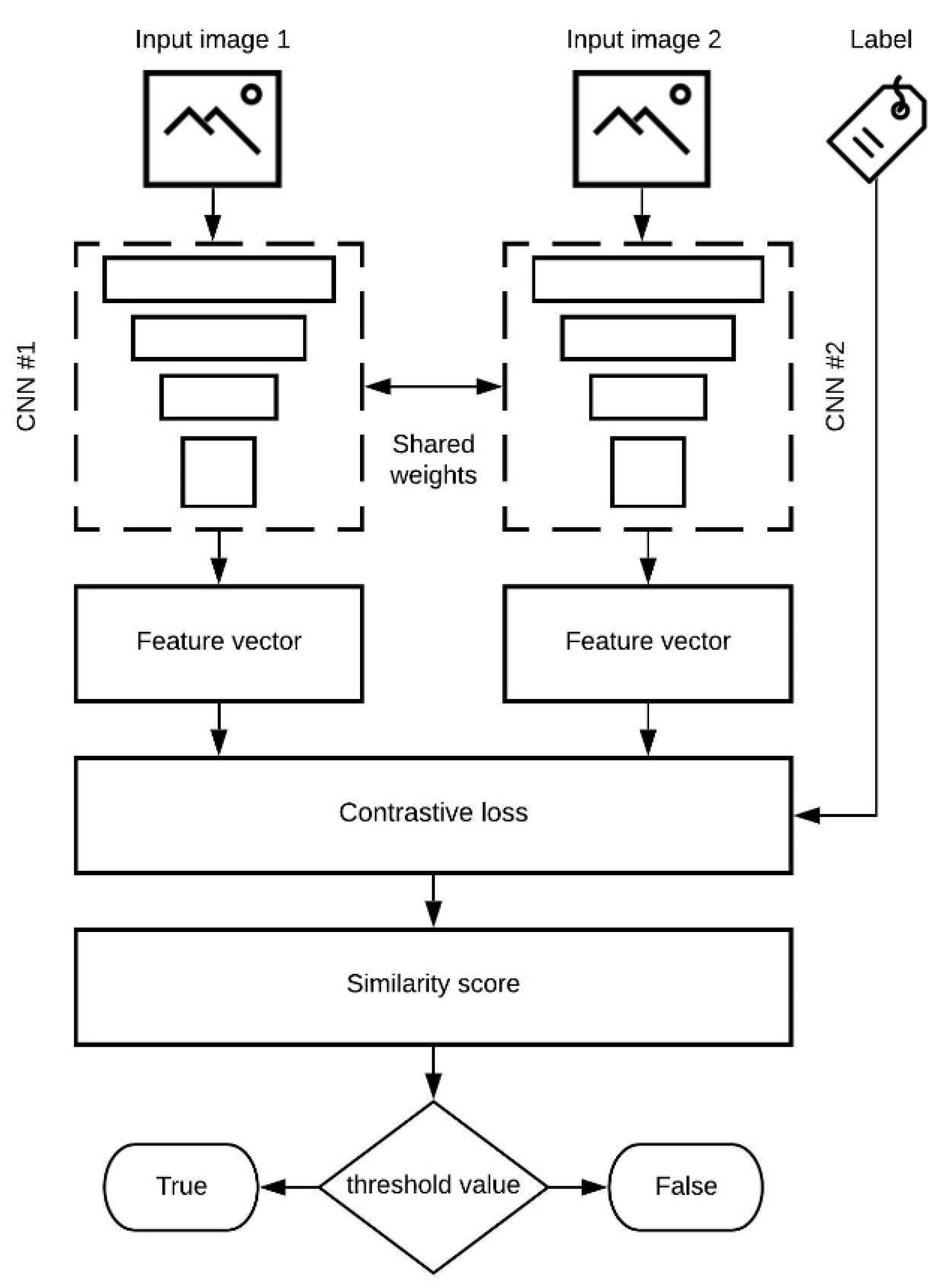
3. The Model
- Can generalize to inputs and outputs that have never been seen before—a network trained on approximately ten classes can also be used on any new class that the network has never seen before, without retraining or changing any parameters;
- Shared weights—two networks with the same configuration and with the same parameters;
- Explainable results—it is easy to notice why the network responded with a high or low similarity score;
- Less overfitting—the network can work with one image per class;
- Labeled data—before training, all data must be labeled and organized;
- Pairwise learning—what makes two inputs similar;
- In terms of dataset size—less is more.
- Computationally intensive—less data but more data-pairs;
- Fine-tuning is necessary—the network layer architecture should be designed for solving a specific problem;
- Quality over quantity—the dataset must be carefully created and inspected;
- Choosing loss function—available loss functions are contrastive loss, triplet loss, magnet loss, and center loss.
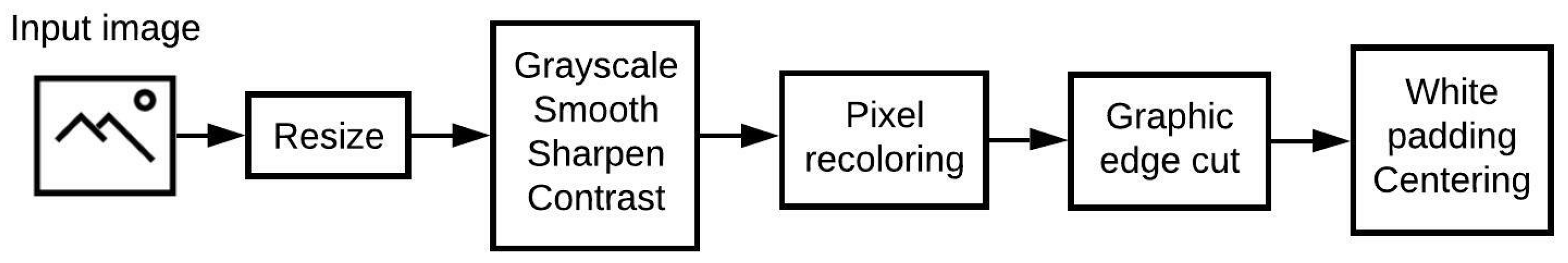
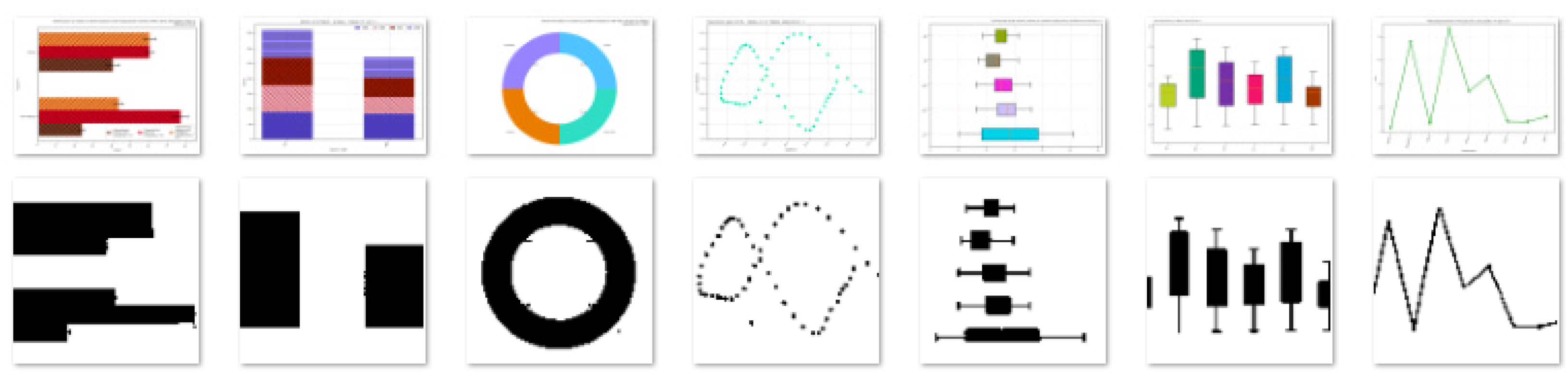
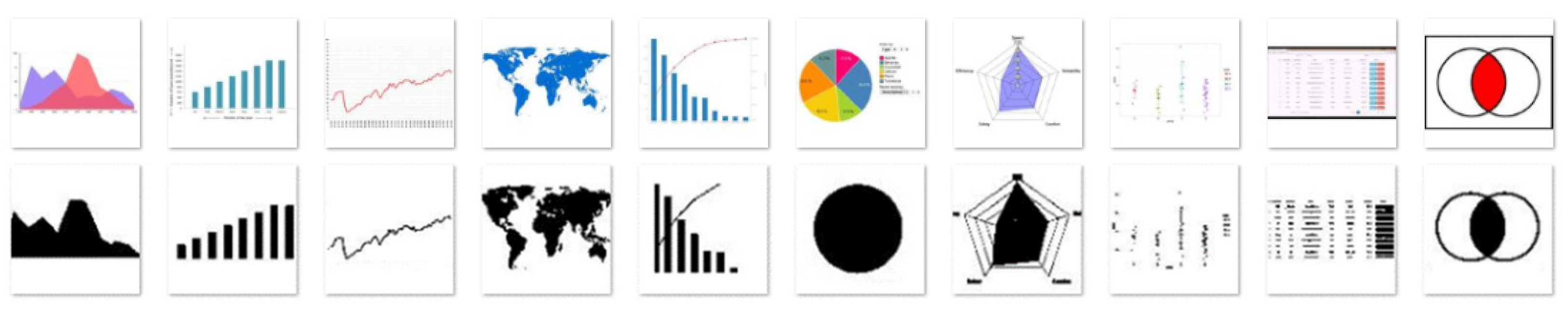
3.1. The Dataset
- AT&T Database of Faces, which consists of 400 images, is divided into 40 classes [31].
3.2. The Architecture
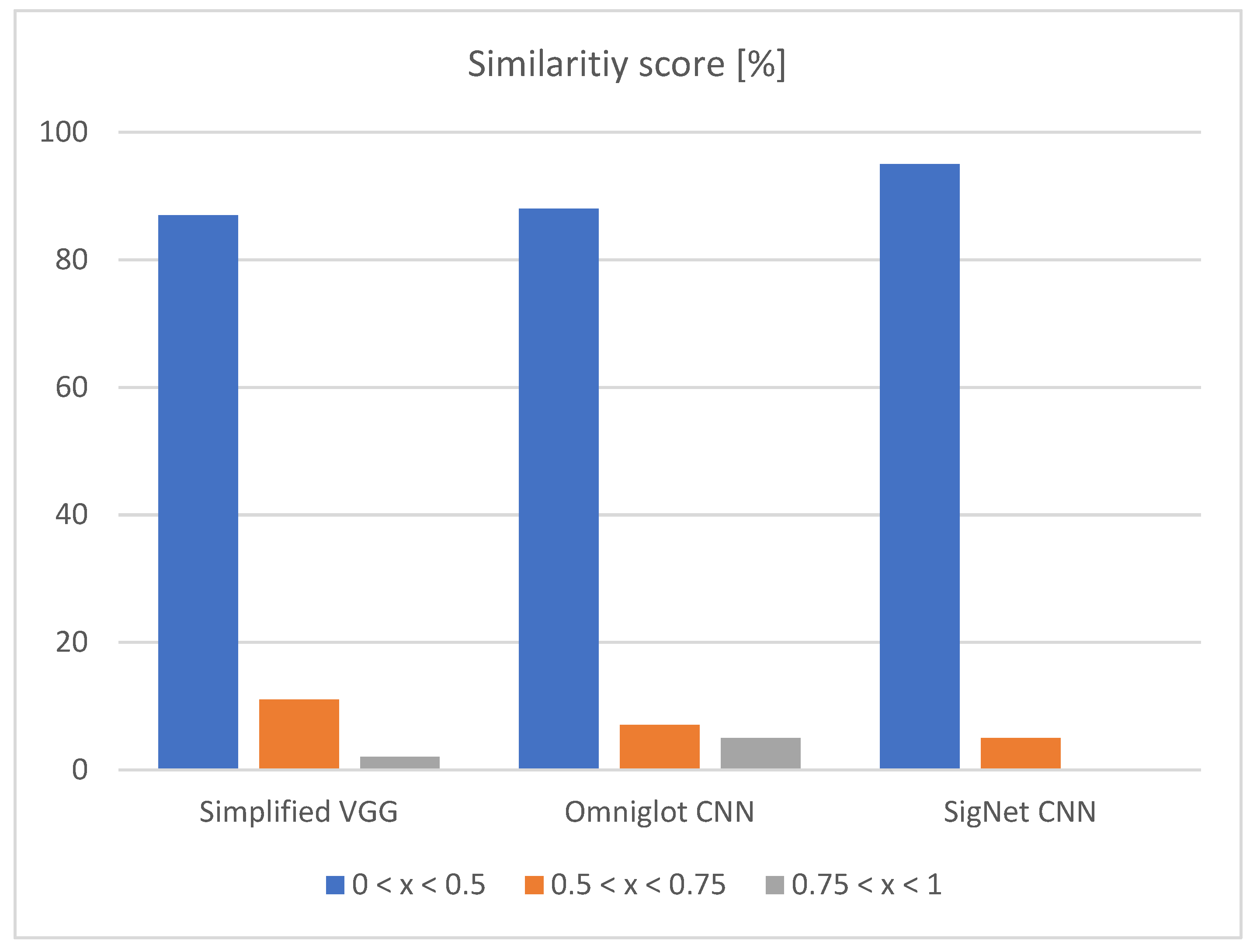
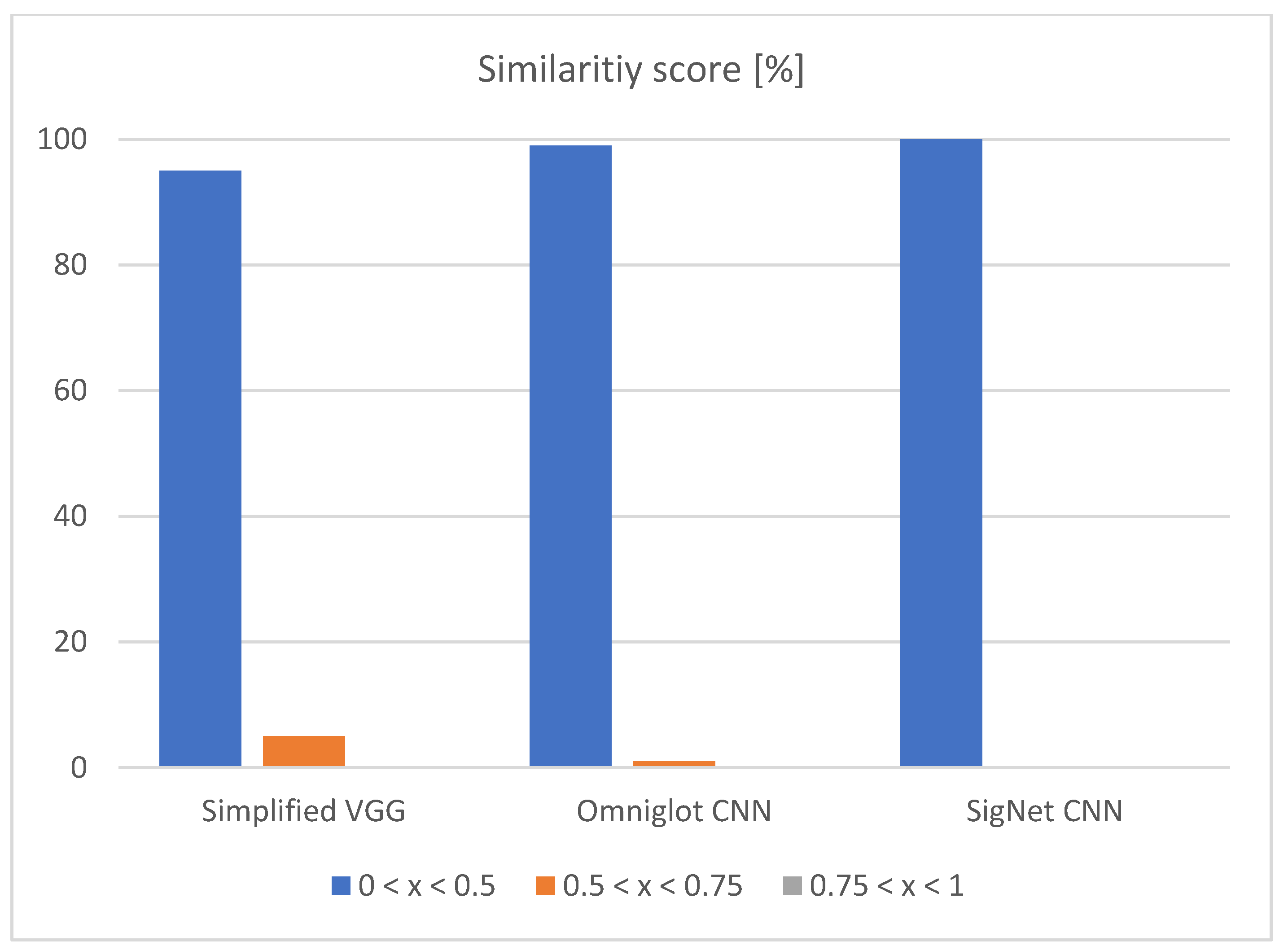
- SigNet CNN—the network used for writer independent offline signature verification. The authors report accuracy ranging from 76% to 100%, depending on the used dataset [26]. The achieved results are for Siamese CNN architecture.
- Omniglot CNN—the network used on the Omniglot dataset for the validation of handwritten characters. The authors report accuracy ranging from 70% to 92%, depending on the used dataset [32]. The achieved results are for Siamese CNN architecture.
3.3. Experiment Setup
4. Experiments
4.1. Verification
4.2. Results
5. Conclusions
Author Contributions
Funding
Institutional Review Board Statement
Informed Consent Statement
Data Availability Statement
Conflicts of Interest
References
- Chen, C.; Härdle, W.; Unwin, A.; Friendly, M. A brief history of data visualization. In Handbook of Data Visualization; Springer: Berlin/Heidelberg, Germany, 2008; pp. 15–56. [Google Scholar]
- Zhou, Y.P.; Tan, C.L. Hough Technique for Bar Charts Detection and Recognition in Document Images. 2000. Available online: https://ieeexplore.ieee.org/abstract/document/899506/ (accessed on 1 May 2020).
- Zhou, Y.P.; Tan, C.L. Bar charts recognition using hough based syntactic segmentation. In Theory and Application of Diagrams; Springer: Berlin/Heidelberg, Germany, 2000; pp. 494–497. [Google Scholar]
- Redeke, I. Image & Graphic Reader. Available online: https://ieeexplore.ieee.org/abstract/document/959168/ (accessed on 1 May 2020).
- Gao, J.; Zhou, Y.; Barner, K.E. View: Visual Information Extraction Widget for Improving Chart Images Accessibility. Available online: https://ieeexplore.ieee.org/abstract/document/6467497/ (accessed on 1 May 2020).
- Battle, L.; Duan, P.; Miranda, Z.; Mukusheva, D.; Chang, R.; Stonebraker, M. Beagle: Automated extraction and interpretation of visualizations from the web. In Proceedings of the Conference on Human Factors in Computing Systems, Montreal, QC, Canada, 21–26 April 2018. [Google Scholar] [CrossRef]
- Mishchenko, A.; Vassilieva, N. Model-Based Recognition and Extraction of Information from Chart Images. Available online: https://pdfs.semanticscholar.org/33c3/2c036fa74d2fe812759e9c3d443767e3fb5b.pdf (accessed on 1 May 2020).
- Mishchenko, A.; Vassilieva, N. Model-Based Chart Image Classification; Lecture Notes in Computer Science (Including subseries Lecture Notes in Artificial Intelligence and Lecture Notes in Bioinformatics); Springer: Berlin/Heidelberg, Germany, 2011; Volume 6939, pp. 476–485. [Google Scholar] [CrossRef]
- Poco, J.; Heer, J. Reverse-engineering visualizations: Recovering visual encodings from chart images. Comput. Graph. Forum 2017, 36, 353–363. [Google Scholar] [CrossRef]
- Savva, M.; Kong, N.; Chhajta, A.; Li, F.F.; Agrawala, M.; Heer, J. ReVision: Automated Classification, Analysis and Redesign of Chart Images. In Proceedings of the UIST’11 24th Annual ACM Symposium on User Interface Software and Technology, Santa Barbara, CA, USA, 16–19 October 2011; pp. 393–402. [Google Scholar] [CrossRef]
- Lin, A.; Ford, J.; Adar, E.; Hecht, B. VizByWiki: Mining Data Visualizations from the Web to Enrich News Articles. Available online: https://dl.acm.org/doi/abs/10.1145/3178876.3186135 (accessed on 1 May 2020).
- Choi, J.; Jung, S.; Park, D.G.; Choo, J.; Elmqvist, N. Visualizing for the Non-visual: Enabling the Visually Impaired to Use Visualization. Comput. Graph. Forum 2019, 38, 249–260. [Google Scholar] [CrossRef]
- Jobin, K.V.; Mondal, A.; Jawahar, C. DocFigure: A Dataset for Scientific Document Figure Classification. Available online: https://researchweb.iiit.ac.in/ (accessed on 1 May 2020).
- Kaur, P.; Kiesel, D. Combining image and caption analysis for classifying charts in biodiversity. In Proceedings of the 15th International Joint Conference on Computer Vision, Imaging and Computer Graphics Theory and Applications—IVAPP, Valletta, Malta, 27–29 February 2020; pp. 157–168. [Google Scholar] [CrossRef]
- Bajić, F.; Job, J.; Nenadić, K. Data visualization classification using simple convolutional neural network model. Int. J. Electr. Comput. Eng. Syst. 2020, 11, 43–51. [Google Scholar] [CrossRef]
- Kosemen, C.; Birant, D. Multi-label classification of line chart images using convolutional neural networks. SN Appl. Sci. 2020, 2, 1250. [Google Scholar] [CrossRef]
- Ishihara, T.; Morita, K.; Shirai, N.C.; Wakabayashi, T.; Ohyama, W. Chart-type classification using convolutional neural network for scholarly figures. In Asian Conference on Pattern Recognition; Springer: Cham, Switzerland, 2019; pp. 252–261. [Google Scholar]
- Dadhich, K.; Daggubati, S.C.; Sreevalsan-Nair, J. BarChartAnalyzer: Digitizing images of bar charts. In Proceedings of the International Conference on Image Processing and Vision Engineering—IMPROVE, Online, 28–30 April 2021. [Google Scholar]
- Zhou, F.; Zhao, Y.; Chen, W.; Tan, Y.; Xu, W.; Chen, Y.; Liu, C.; Zhao, Y. Reverse-engineering bar charts using neural networks. J. Vis. 2021, 24, 419–435. [Google Scholar] [CrossRef]
- Chagas, P.; Freitas, A.; Daisuke, R.; Miranda, B.; Araujo, T.; Santos, C.; Meiguins, B.; Morais, J. Architecture Proposal for Data Extraction of Chart Images Using Convolutional Neural Network. Available online: https://ieeexplore.ieee.org/abstract/document/8107990/ (accessed on 1 May 2020).
- Huang, S. An Image Classification Tool of Wikimedia Commons. Available online: https://edoc.hu-berlin.de/handle/18452/22325 (accessed on 30 August 2020).
- Dai, W.; Wang, M.; Niu, Z.; Zhang, J. Chart decoder: Generating Textual and Numeric Information from Chart Images Automatically. Available online: https://www.sciencedirect.com/science/article/pii/S1045926X18301162 (accessed on 1 May 2020).
- Thiyam, J.; Singh, S.R.; Bora, P.K. Challenges in chart image classification: A comparative study of different deep learning methods. In Proceedings of the 21st ACM Symposium on Document Engineering, Limerick, Ireland, 24–27 August 2021. [Google Scholar]
- Bromley, J.; Guyon, I.; LeCun, Y.; Sackinger, E.; Shash, R. Signature verification using a siamese time delay neural network. Int. J. Pattern Recognit. Artif. Intell. 1993, 7, 669–688. [Google Scholar] [CrossRef] [Green Version]
- Song, L.; Gong, D.; Li, Z.; Liu, C.; Liu, W. Occlusion robust face recognition based on mask learning with pairwise differential siamese network. In Proceedings of the IEEE/CVF International Conference on Computer Vision, Seoul, Korea, 27 October–2 November 2019; pp. 773–782. [Google Scholar]
- Dey, S.; Dutta, A.; Toledo, J.I.; Ghosh, S.K.; Lladós, J.; Pal, U. Signet: Convolutional Siamese network for writer independent offline signature verification. arXiv 2017, arXiv:1707.02131. [Google Scholar]
- Langford, Z.; Eisenbeiser, L.; Vondal, M. Robust signal classification using siamese networks. In Proceedings of the ACM Workshop on Wireless Security and Machine Learning, Miami, FL, USA, 15–17 May 2019; pp. 1–5. [Google Scholar]
- Lian, Z.; Li, Y.; Tao, J.; Huang, J. Speech emotion recognition via contrastive loss under siamese networks. In Proceedings of the Joint Workshop of the 4th Workshop on Affective Social Multimedia Computing and First Multi-Modal Affective Computing of Large-Scale Multimedia Data, Seoul, Korea, 26 October 2018; pp. 21–26. [Google Scholar]
- Bajić, F.; Job, J.; Nenadić, K. Chart classification using simplified VGG model. In Proceedings of the 2019 International Conference on Systems, Signals and Image Processing (IWSSIP), Osijeka, Croatia, 5–7 June 2019. [Google Scholar]
- Tensmeyer, C. Competition on Harvesting Raw Tables (CHART) 2019-Synthetic (CHART2019-S), 1, ID: CHART2019-S_1. Available online: http://tc11.cvc.uab.es/datasets/CHART2019-S_1 (accessed on 15 November 2020).
- AT&T Laboratories Cambridge. The Database of Faces 2002. Available online: http://www.cl.cam.ac.uk/research/dtg/attarchive/facedatabase.html (accessed on 17 November 2020).
- Koch, G.; Zemel, R.; Salakhutdinov, R. Siamese neural networks for one-shot image recognition. In Proceedings of the ICML Deep Learning Workshop, Lille, France, 10–11 July 2015; Volume 2. [Google Scholar]
- Lake, B.M.; Salakhutdinov, R.; Gross, J.; Tenenbaum, J.B. One shot learning of simple visual concepts. In Proceedings of the 33rd Annual Conference of the Cognitive Science Society, Boston, MA, USA, 20–23 July 2011; Volume 172. [Google Scholar]


| Ref. | Year | Method | Results CA—Classification Accuracy DE—Data Extraction | Dataset |
|---|---|---|---|---|
| [2] | 2000 | Modified Probabilistic Hough Transform | Bar reconstruction rate 92.30%. Correlation of bar pattern and text 87.30% | 20 |
| [3] | 2000 | Modified Probabilistic Hough Transform | CA: synthetic bar 90.00%, real images of a bar 87.30%, hand-draw bar 78.00% | 35 |
| [4] | 2001 | Custom algorithm | CA: bar 73.00%, pie 93.00% | 55 |
| [7] | 2011 | Model-based | CA: line 100.00%, area 96.00%, bar 96.00%, 2D pie 74.00%, 3D pie 85.00% | 980 |
| [8] | 2011 | Model-based | CA: line 100.00%, area 96.00%, bar 96.00%, 2D pie 74.00%, 3D pie 85.00% | 980 |
| [10] | 2011 | SVM | CA: area 88.00%, bar 78.00, line 73.00%, map 84.00%, Pareto 85.00%, pie 79.00%, radar 88.00%, scatter 79.00%, Table 86.00%, Venn 75.00%. | 2601 |
| [5] | 2012 | Custom algorithm, SVM | CA: 97.00% (bar, pie, line) | 300 |
| [9] | 2017 | CNN, SVM | CA: area 95.00%, bar 97.00%, line 94.00%, map 96.00%, Pareto 89.00%, pie 98.00%, radar 93.00%, scatter 92.00%, Table 98.00%, Venn 91.00% | 5125 |
| [20] | 2017 | CNN | CA: 70.00% (area, bar, line, map, Pareto, pie, radar, scatter, table, Venn) | 4837 |
| [6] | 2018 | Custom algorithm | CA: from 83.10% to 94.00% | 33,778 |
| [11] | 2018 | CNN | CA: non-dataviz 89.00%, dataviz 93.00% | 755 |
| [22] | 2018 | CNN | CA: 99%. (bar, pie, line, scatter, radar) DE: from 77.00% to 89.00%. | 11,174 |
| [12] | 2019 | CNN | CA: area 96.00%, bar 98.00%, line 99.00%, map 97.00%, Pareto 100.00%, pie 96.00%, radar 94.00%, scatter 98.00%, Table 92.00%, Venn 97.00%. DE: 87.67%. | 2398 |
| [13] | 2019 | CNN | CA: 28 types from 88.96% to 92.90% | 33,000 |
| [14] | 2020 | CNN | CA: ordination 98.00%, map 97.00%, scatter 89.00%, line 91.00%, dendogram 97.00%, column 97.00%, heat map 95.00%, box 96.00%, area 80.00%, network 91.00%, histogram 83.00%, timeseries 84.00%, pie 97.00%, stack area 96.00% | 4073 |
| [15] | 2020 | CNN | Comparison of image preprocessing methods to overall chart classification | 3002 |
| [16] | 2020 | CNN | CA: line 93.75% | 1920 |
| [17] | 2020 | CNN | CA: line 97.00% | 4718 |
| [21] | 2020 | CNN | Comparison of pre-trained and fine-tuned models | 4249 |
| [18] | 2021 | CNN | CA: bar 85% | 1400 |
| [19] | 2021 | CNN | DE: bar 85% | 30,480 |
| [23] | 2021 | CNN | Comparison of deep learning models | 57,097 |
| Dataset 1 | ||
| Chart type | Available | Validation Set |
| Area | 288 | 20 |
| Bar | 301 | 20 |
| Line | 267 | 20 |
| Map | 126 | 20 |
| Pareto | 208 | 20 |
| Pie | 422 | 20 |
| Radar | 381 | 20 |
| Scatter | 268 | 20 |
| Table | 383 | 20 |
| Venn | 158 | 20 |
| Total | 2802 | 200 |
| 3002 | ||
| Dataset 2 | ||
| Chart type | Available | Validation Set |
| Pie | 28,183 | 20 |
| Line | 41,854 | 20 |
| Scatter | 41,683 | 20 |
| Horizontal box | 20,987 | 20 |
| Vertical box | 20,938 | 20 |
| Horizontal bar | 22,284 | 20 |
| Vertical bar | 21,941 | 20 |
| Total | 197,870 | 140 |
| 198,010 | ||
| Image Pair (Class N) | Input Image 1 (New Image) | Input Image 2 (Known Image) | Similarity Score (SS) |
|---|---|---|---|
| 1 |  |  | SS1 |
| 2 |  |  | SS2 |
| 3 |  |  | SS3 |
| 4 |  |  | SS4 |
| 5 |  |  | SS5 |
| 6 |  |  | SS6 |
| 7 |  |  | SS7 |
| 8 |  |  | SS8 |
| 9 |  |  | SS9 |
| 10 |  |  | SS10 |
| Input vs. Random Train Image from Each Class | Input vs. Highest Similarity Image from Each Class | |||||
|---|---|---|---|---|---|---|
| Simplified VGG | Omniglot CNN | SigNet CNN | Simplified VGG | Omniglot CNN | SigNet CNN | |
| Accuracy (%) | 68.00 | 40.00 | 30.00 | 82.00 | 63.00 | 41.00 |
| Precision (%) | 68.00 | 39.50 | 29.50 | 81.50 | 63.00 | 40.50 |
| Recall (%) | 69.36 | 46.32 | 29.83 | 84.24 | 66.67 | 42.34 |
| F-1 score (%) | 67.86 | 39.68 | 29.43 | 81.94 | 63.00 | 40.54 |
| p < 0.05 | H0 | |
|---|---|---|
| input vs. random train image from each class | ||
| Simplified VGG—Omniglot CNN | true | reject |
| Simplified VGG—SigNet CNN | true | reject |
| Omniglot CNN—SigNet CNN | true | reject |
| input vs. highest similaritiy image from each class | ||
| Simplified VGG—Omniglot CNN | true | reject |
| Simplified VGG—SigNet CNN | true | reject |
| Omniglot CNN—SigNet CNN | true | reject |
| Simplified VGG | Seen Classes during Network Training | Unseen Class | Accuracy (%) | |||||||||
|---|---|---|---|---|---|---|---|---|---|---|---|---|
| Area | Bar | Line | Map | Pareto | Pie | Radar | Scatter | Table | Venn | Box | ||
| Area | 15 (16) | 5 (4) | - | - | - | - | - | - | - | - | - | 75 (80) |
| Bar | - | 15 (16) | - | - | 5 (4) | - | - | - | - | - | - | 75 (80) |
| Line | - | - | 16 (16) | - | - | - | - | 4 (4) | - | - | - | 80 (80) |
| Map | 5 (6) | - | - | 10 (14) | - | - | - | - | - | 5 (0) | - | 50 (70) |
| Pareto | - | 3 (3) | 2 (0) | - | 15 (17) | - | - | - | - | - | - | 75 (85) |
| Pie | - | - | - | - | - | 17 (20) | - | - | - | 3 (0) | - | 85 (100) |
| Radar | - | - | 4 (4) | - | - | - | 13 (16) | 3 (0) | - | - | - | 65 (80) |
| Scatter | - | - | 3 (4) | - | - | - | 4 (0) | 11 (16) | 2 (0) | - | - | 55 (80) |
| Table | - | - | - | - | - | - | 5 (0) | 3 (6) | 12 (14) | - | - | 60 (70) |
| Venn | - | - | - | 2 (0) | - | 6 (2) | - | - | - | 12 (18) | - | 60 (90) |
| Box | - | - | 4 (2) | 8 (0) | - | - | 4 (2) | - | - | - | 4 (16) | 20 (80) |
| (a) input vs. random train image from each class | ||||||||||||
| 10—type classification (without box plot) average: | Precision | 68.00% | Recall | 69.36% | F-1 score | 67.86% | Accuracy | 68.00% | ||||
| 11—type classification (with box plot) average: | Precision | 63.64% | Recall | 67.49% | F-1 score | 62.57% | Accuracy | 64.00% | ||||
| (b) input vs. highest similarity image from each class | ||||||||||||
| 10—type classification (without box plot) average: | Precision | 81.50% | Recall | 84.24% | F-1 score | 81.94% | Accuracy | 82.00% | ||||
| 11—type classification (with box plot) average: | Precision | 81.36% | Recall | 84.19% | F-1 score | 81.86% | Accuracy | 81.00% | ||||
| Dataset | Simplified VGG as Siamese CNN | Simplified VGG as Classic CNN | |||||||||||||||
|---|---|---|---|---|---|---|---|---|---|---|---|---|---|---|---|---|---|
| Input vs. Random Image from Each Class | Input vs. Highest Similarity Image from Each Class | ||||||||||||||||
| Image pairs | Time to classify | Accuracy (%) | Precision (%) | Recall (%) | F-1 score (%) | Image pairs (s) | Time to classify | Accuracy (%) | Precision (%) | Recall (%) | F-1 score (%) | Time to classify | Accuracy (%) | Precision (%) | Recall (%) | F-1 score (%) | |
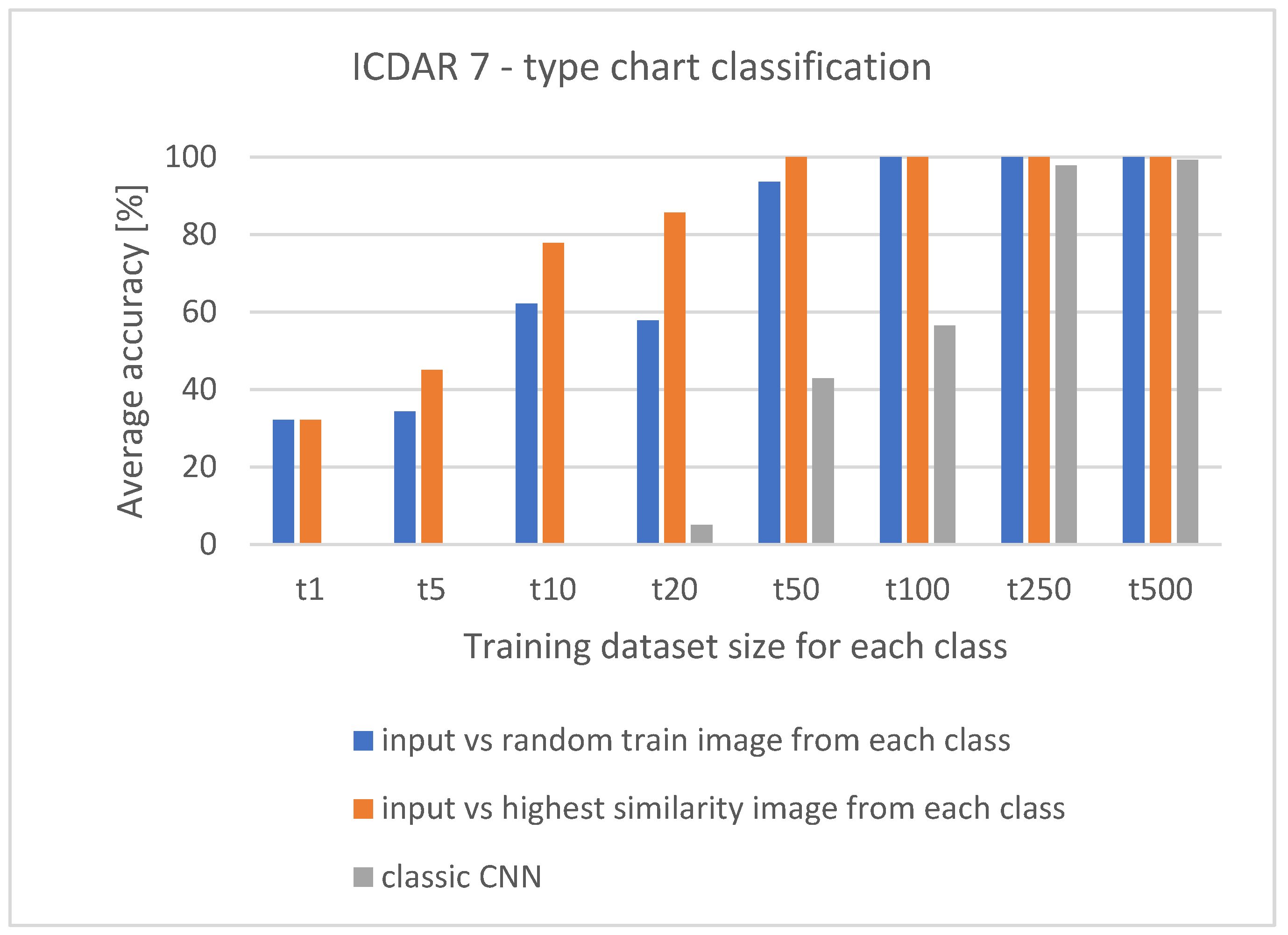
| t1 | 140 | 2 s | 32.14 | 32.14 | 40.46 | 32.45 | 140 | 2 s | 32.14 | 32.14 | 40.46 | 32.45 | 1 s | 0 | 0 | 0 | 0 |
| t5 | 140 | 2 s | 34.28 | 34.28 | 41.47 | 35.36 | 700 | 7 s | 45.00 | 45.00 | 49.30 | 46.10 | 1 s | 0 | 0 | 0 | 0 |
| t10 | 140 | 2 s | 62.14 | 62.14 | 64.39 | 62.53 | 1400 | 15 s | 77.85 | 77.85 | 78.91 | 78.66 | 1 s | 0 | 0 | 0 | 0 |
| t20 | 140 | 2 s | 57.85 | 57.85 | 60.65 | 57.45 | 2800 | 30 s | 85.71 | 85.71 | 86.60 | 85.62 | 1 s | 5.00 | 5.00 | 15.99 | 5.85 |
| t50 | 140 | 2 s | 93.57 | 93.57 | 94.28 | 94.28 | 7000 | 1 m | 100 | 100 | 100 | 100 | 1 s | 42.85 | 42.85 | 48.22 | 44.87 |
| t100 | 140 | 2 s | 100 | 100 | 100 | 100 | 14,000 | 2 m | 100 | 100 | 100 | 100 | 1 s | 56.42 | 56.42 | 57.70 | 56.63 |
| t250 | 140 | 2 s | 100 | 100 | 100 | 100 | 35,000 | 5 m | 100 | 100 | 100 | 100 | 1 s | 97.85 | 97.85 | 98.70 | 98.56 |
| t500 | 140 | 2 s | 100 | 100 | 100 | 100 | 70,000 | 10 m | 100 | 100 | 100 | 100 | 1 s | 99.28 | 99.28 | 99.32 | 99.28 |
| Dataset | Input vs. Random Image from Each Class—Input vs. Highest Similarity Image from Each Class | Input vs. Random Image from Each Class—Classic CNN | Input vs. Highest Similarity Image from Each Class—Classic CNN | |||
|---|---|---|---|---|---|---|
| p < 0.05 | H0 | p < 0.05 | H0 | p < 0.05 | H0 | |
| t1 | false | failed | true | reject | true | reject |
| t5 | true | reject | true | reject | true | reject |
| t10 | true | reject | true | reject | true | reject |
| t20 | true | reject | true | reject | true | reject |
| t50 | true | reject | true | reject | true | reject |
| t100 | false | failed | true | reject | true | reject |
| t250 | false | failed | false | failed | false | failed |
| t500 | false | failed | false | failed | false | failed |
Publisher’s Note: MDPI stays neutral with regard to jurisdictional claims in published maps and institutional affiliations. |
© 2021 by the authors. Licensee MDPI, Basel, Switzerland. This article is an open access article distributed under the terms and conditions of the Creative Commons Attribution (CC BY) license (https://creativecommons.org/licenses/by/4.0/).
Share and Cite
Bajić, F.; Job, J. Chart Classification Using Siamese CNN. J. Imaging 2021, 7, 220. https://doi.org/10.3390/jimaging7110220
Bajić F, Job J. Chart Classification Using Siamese CNN. Journal of Imaging. 2021; 7(11):220. https://doi.org/10.3390/jimaging7110220
Chicago/Turabian StyleBajić, Filip, and Josip Job. 2021. "Chart Classification Using Siamese CNN" Journal of Imaging 7, no. 11: 220. https://doi.org/10.3390/jimaging7110220
APA StyleBajić, F., & Job, J. (2021). Chart Classification Using Siamese CNN. Journal of Imaging, 7(11), 220. https://doi.org/10.3390/jimaging7110220