Breast Density Classification Using Local Quinary Patterns with Various Neighbourhood Topologies †

 ,
, 
Abstract
1. Introduction
- To the best of our knowledge, this is the first study attempting to use local patterns extracted using the LQP operators in the application of breast density classification.
- We investigate the effects of the local pattern information when obtained using different resolutions, various neighbourhood topologies, different orientations and different dominant local patterns.
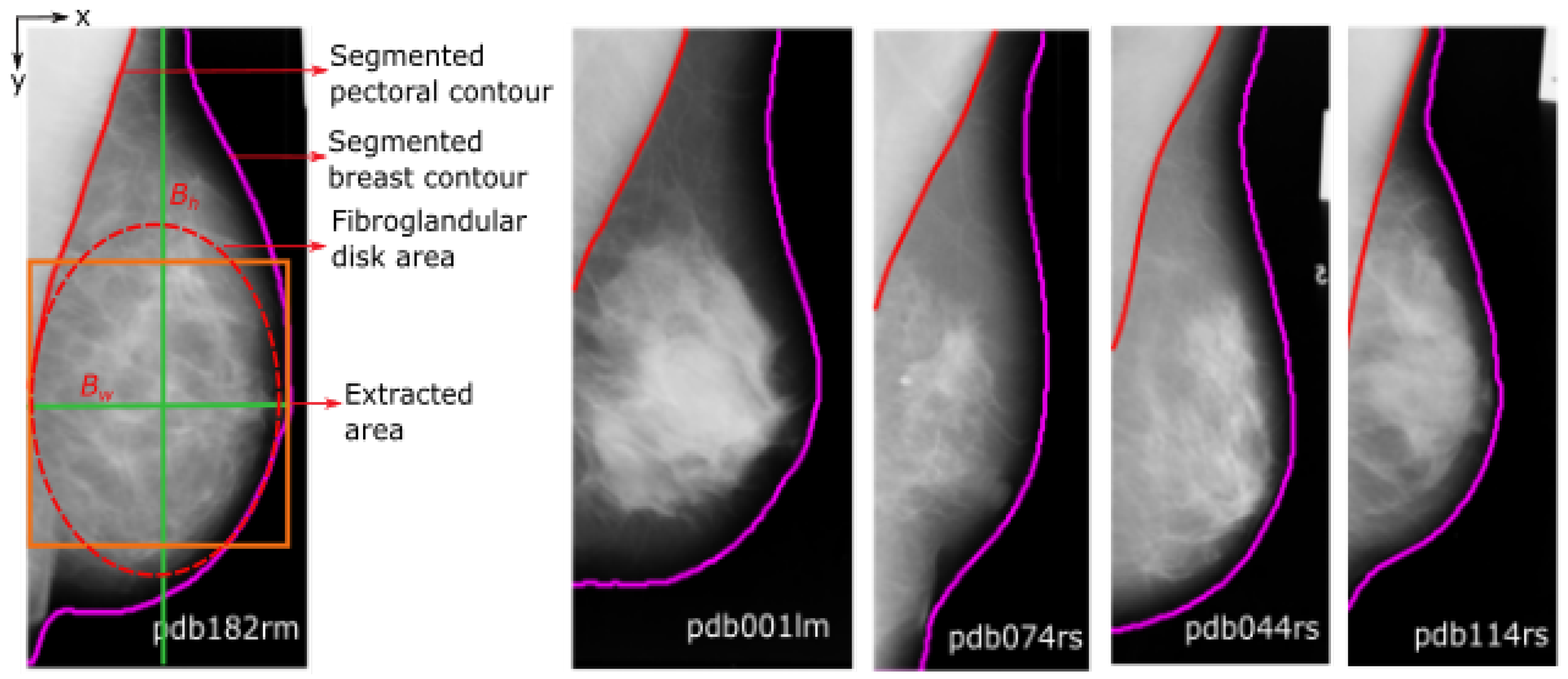
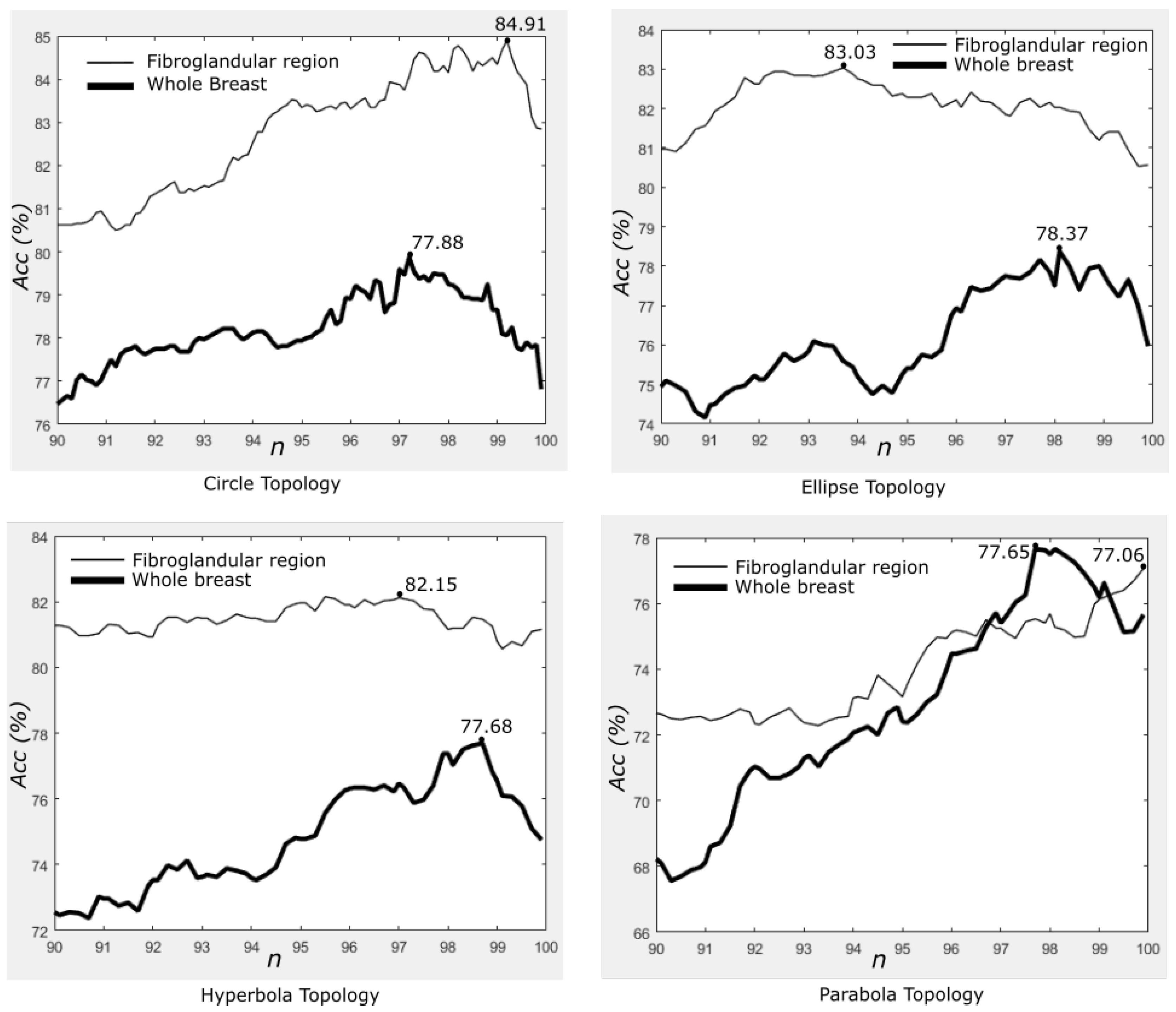
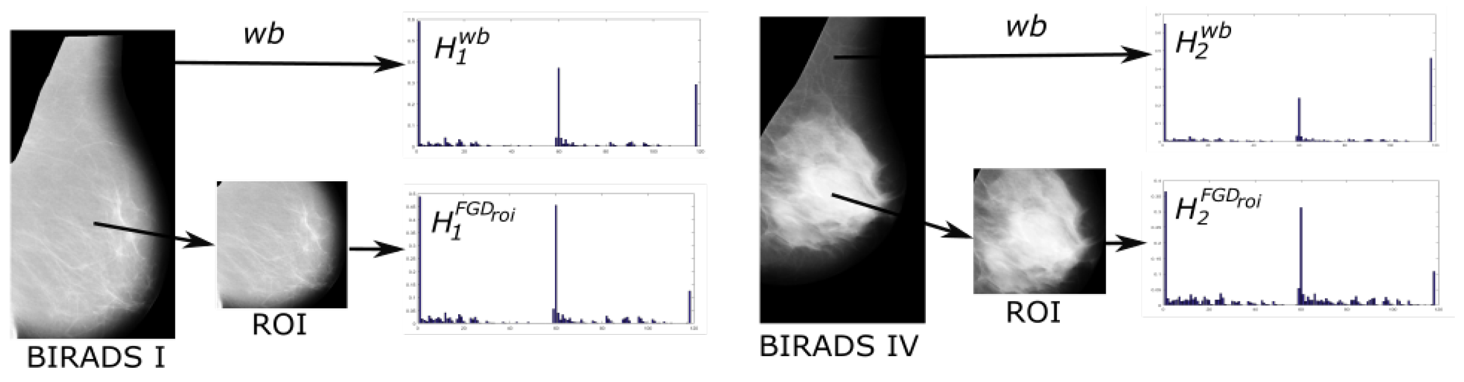
- We show the importance of extracting features from the fibro-glandular region instead of from the whole breast area as all of the current studies in the literature have done.
- We have made a significant extension to the literature review of this study.
- We have extended the evaluation results for the circle topology, which was originally presented in [14] covering different aspects such as parameter selection, orientations and quantitative comparison.
- We investigate the topology aspect of the proposed method such as ellipse, parabola and hyperbola.
- We further evaluated the proposed method on the InBreast [15] dataset.
2. Literature Review
3. Methodology
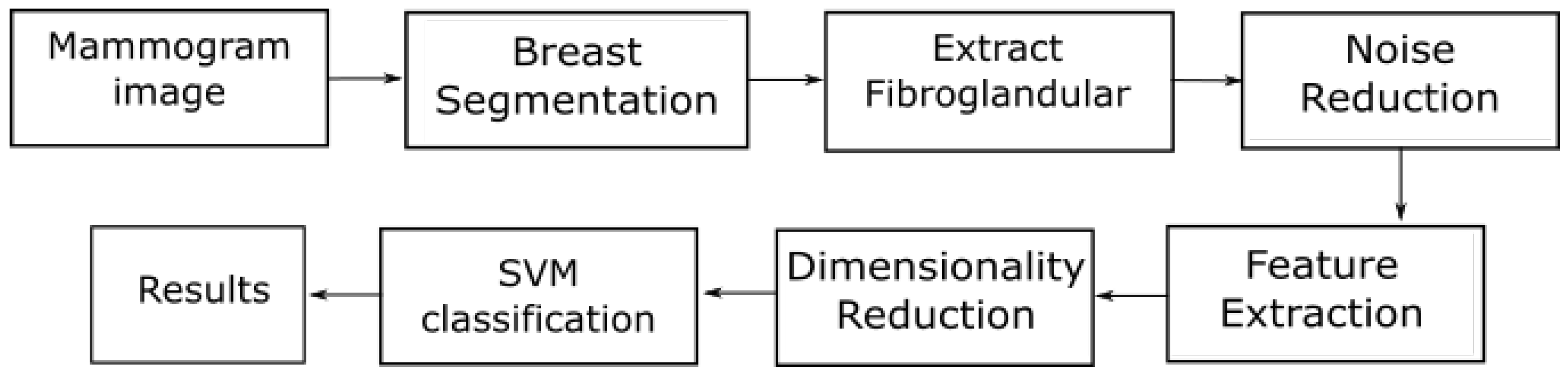
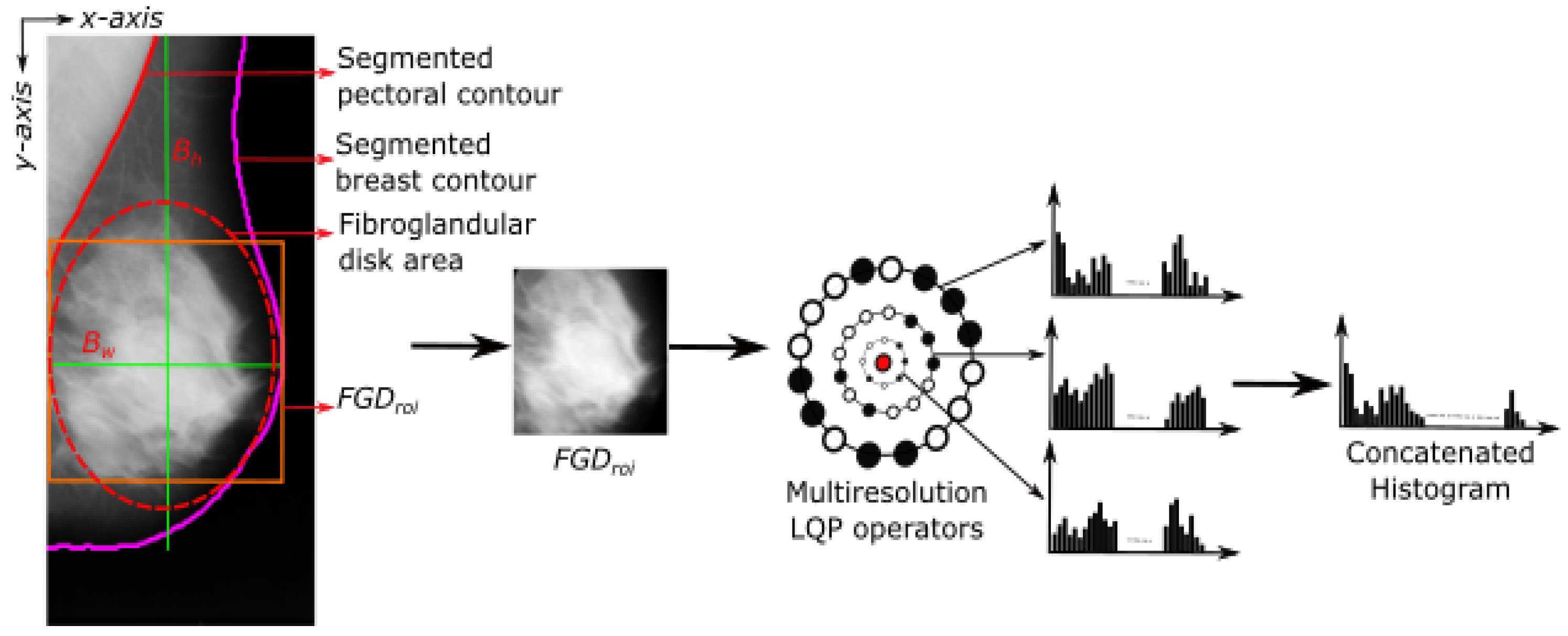
3.1. Pre-Processing
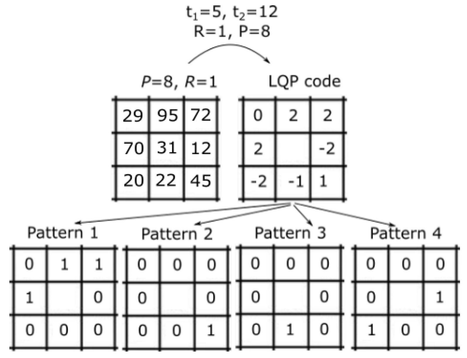
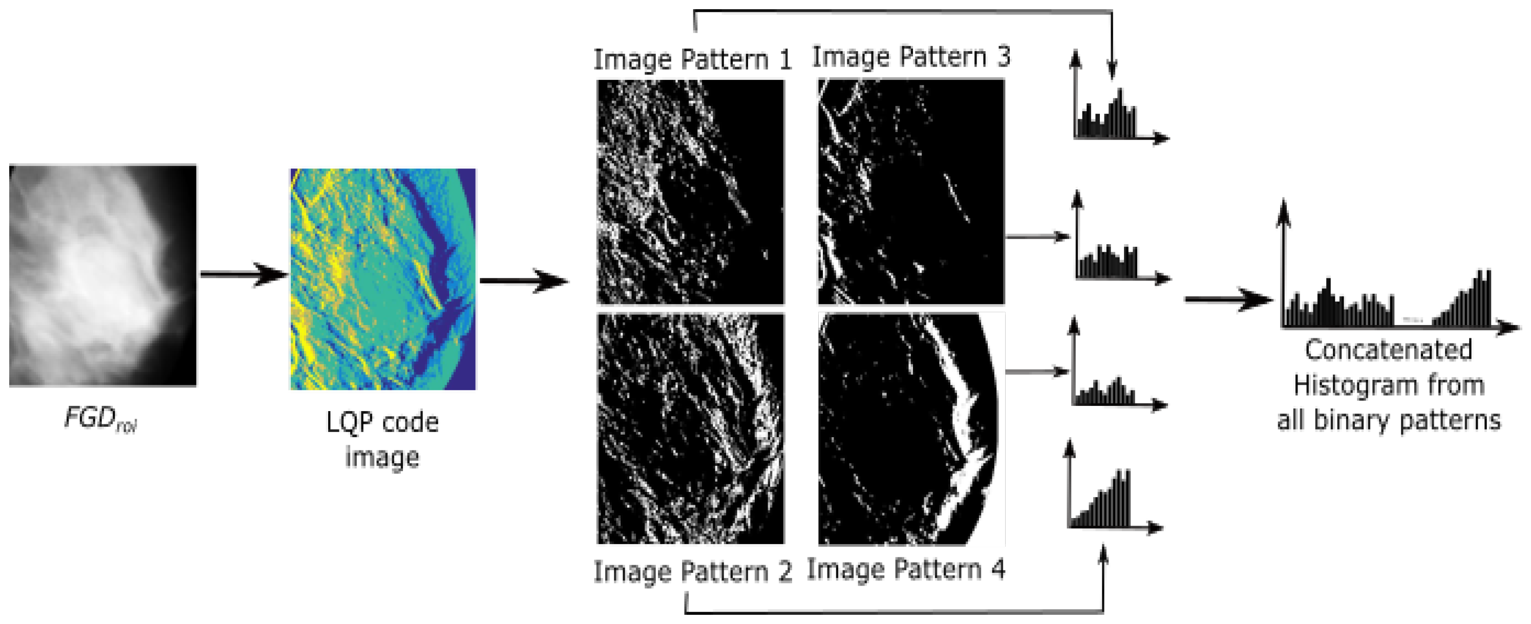
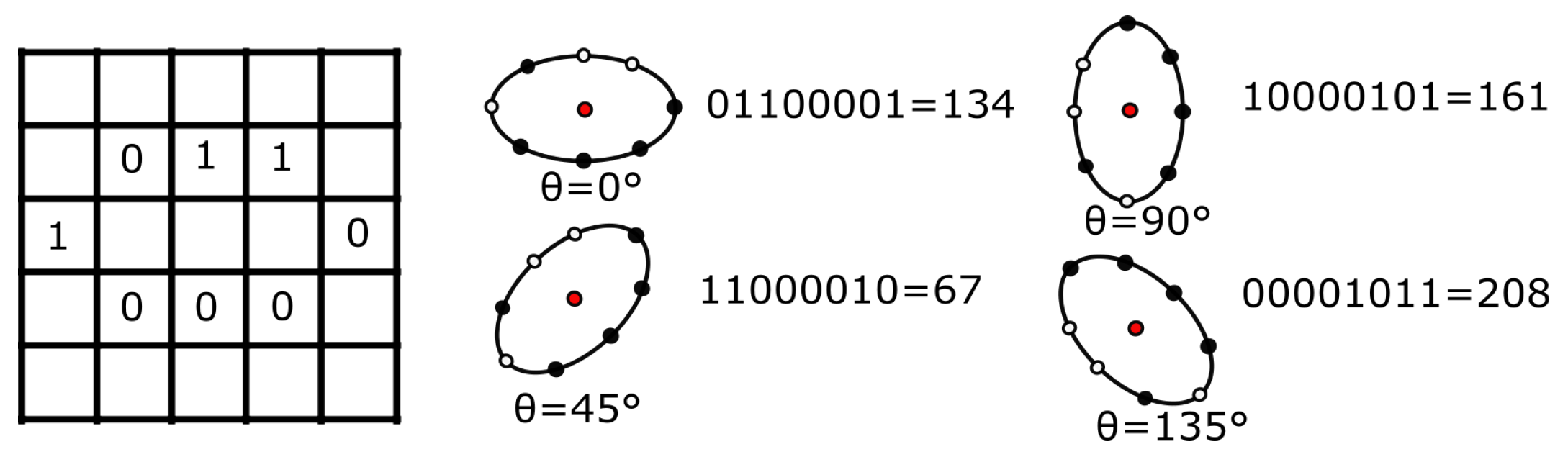
3.2. Feature Extraction
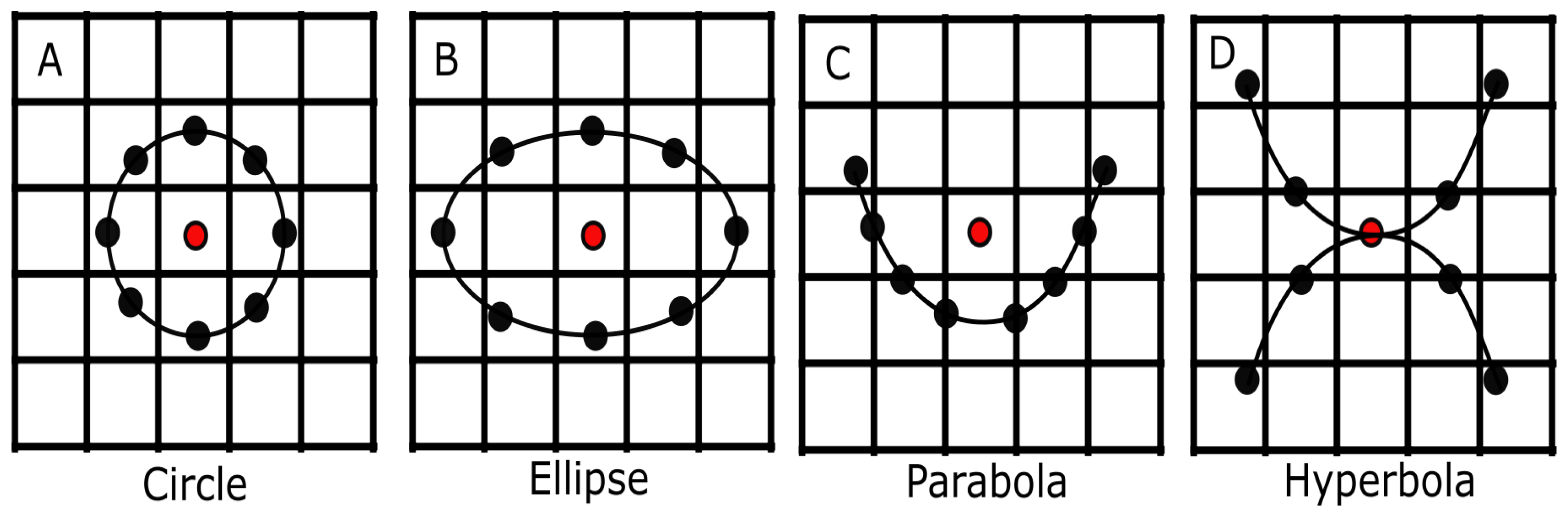
3.3. Neighbourhood Topology
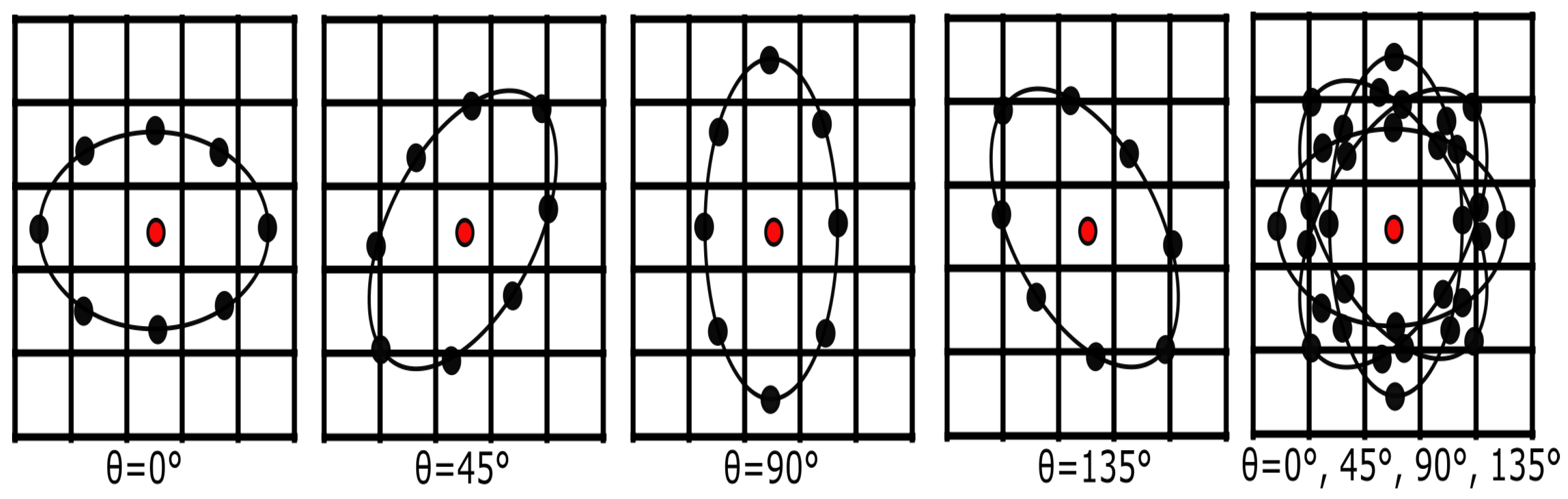
3.4. Topology Orientations
3.5. Dominant Patterns
3.6. Classification
4. Experimental Results
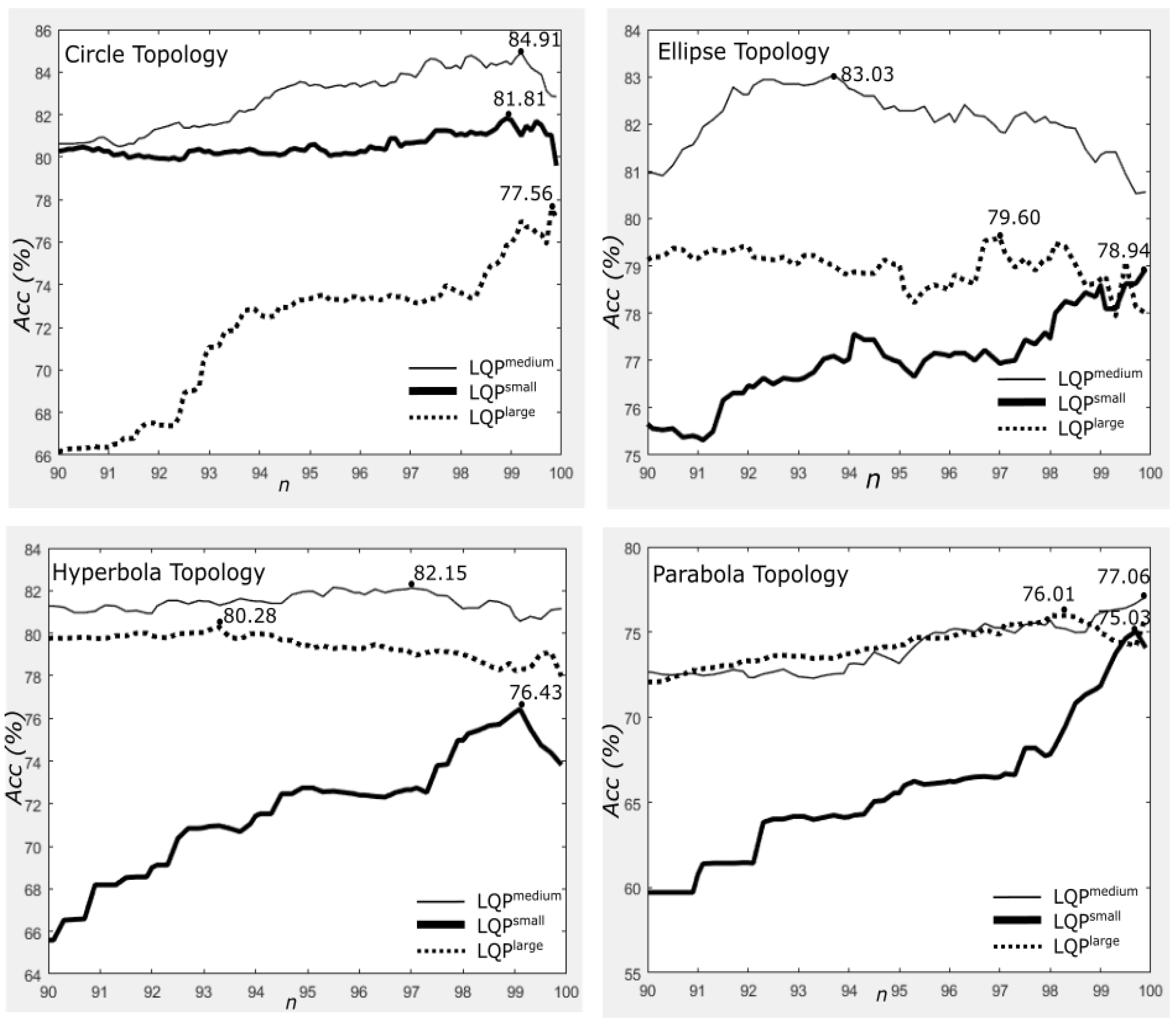
4.1. Results on Different Multiresolutions
- Small multiresolution (),
- Medium multiresolution (),
- Large multiresolution ().
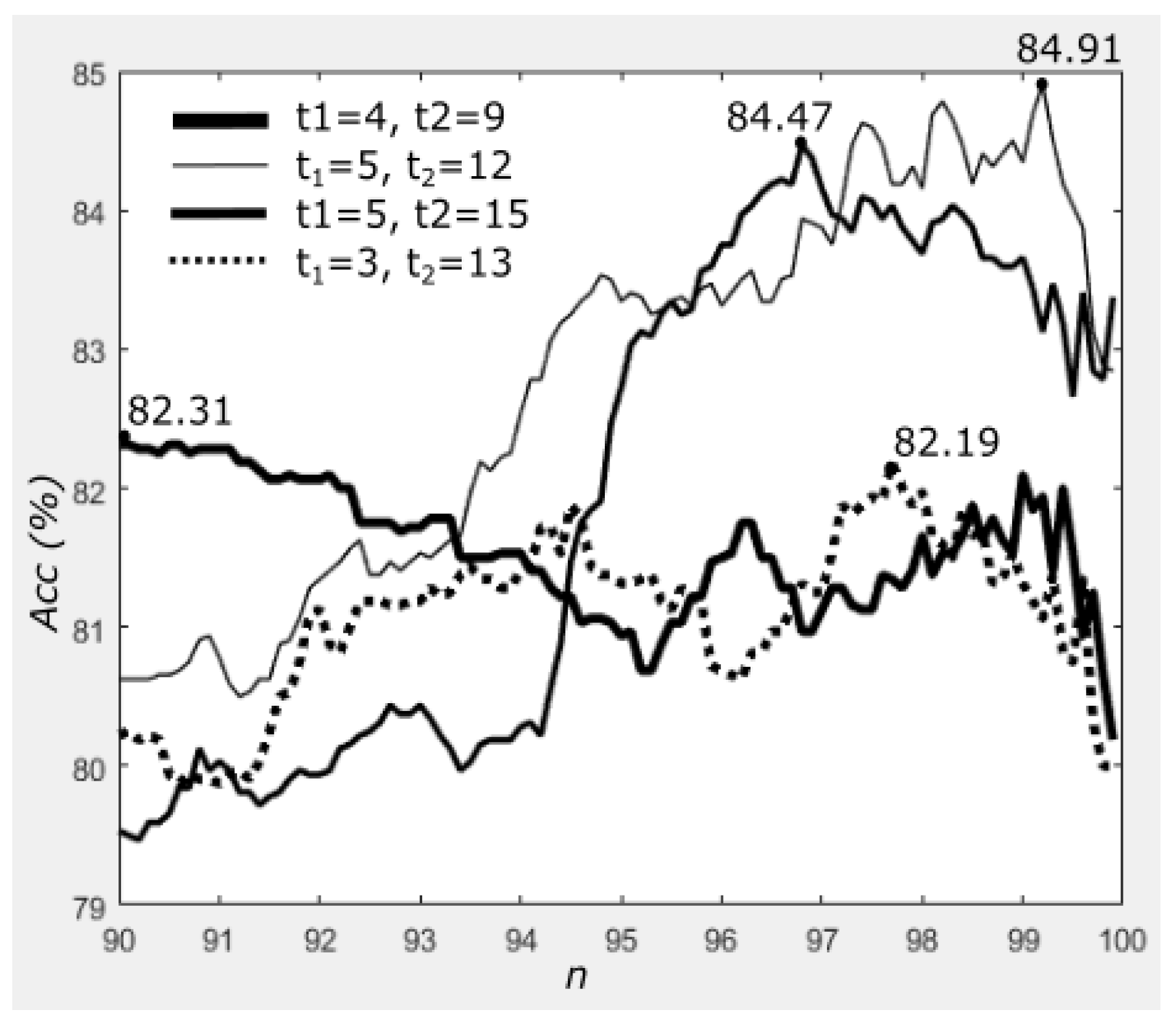
4.2. Results on Different Thresholds
4.3. Fibro-Glandular Region versus Whole Breast Region
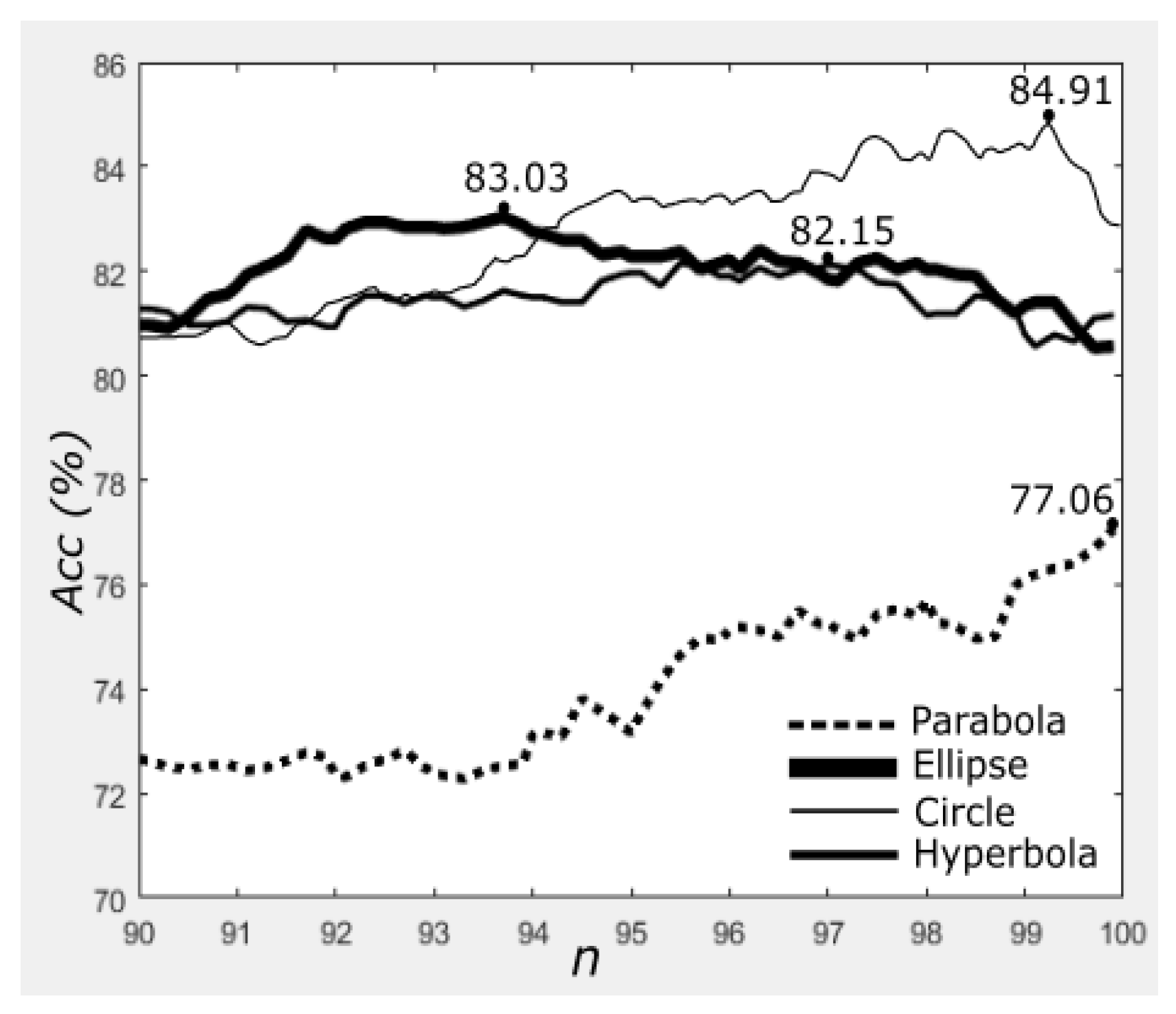
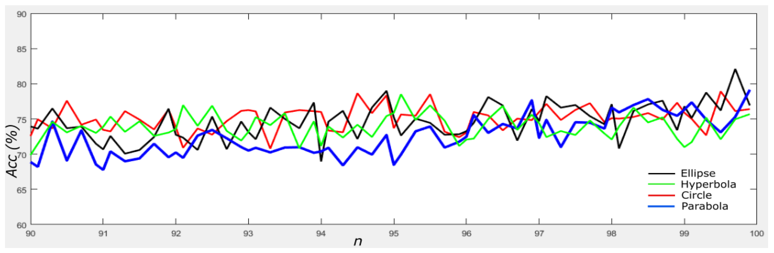
4.4. Results on Different Neighbourhood Topologies
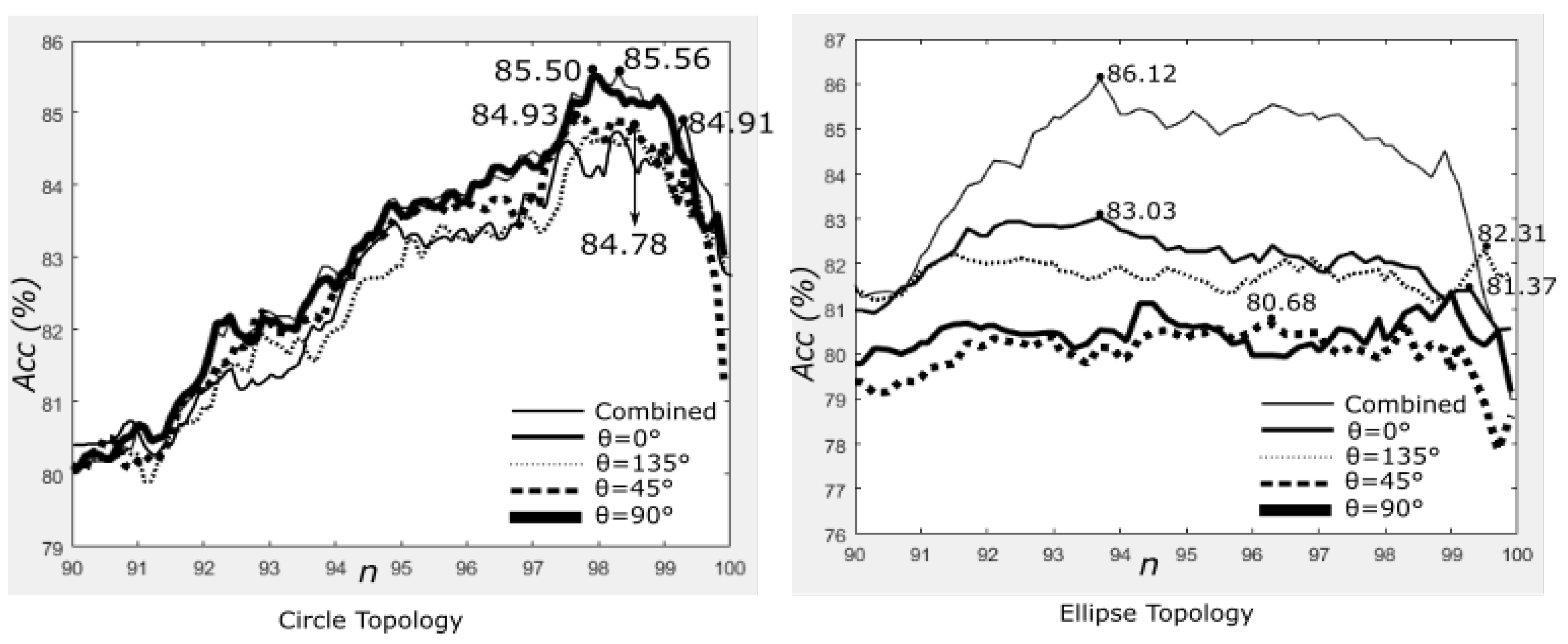
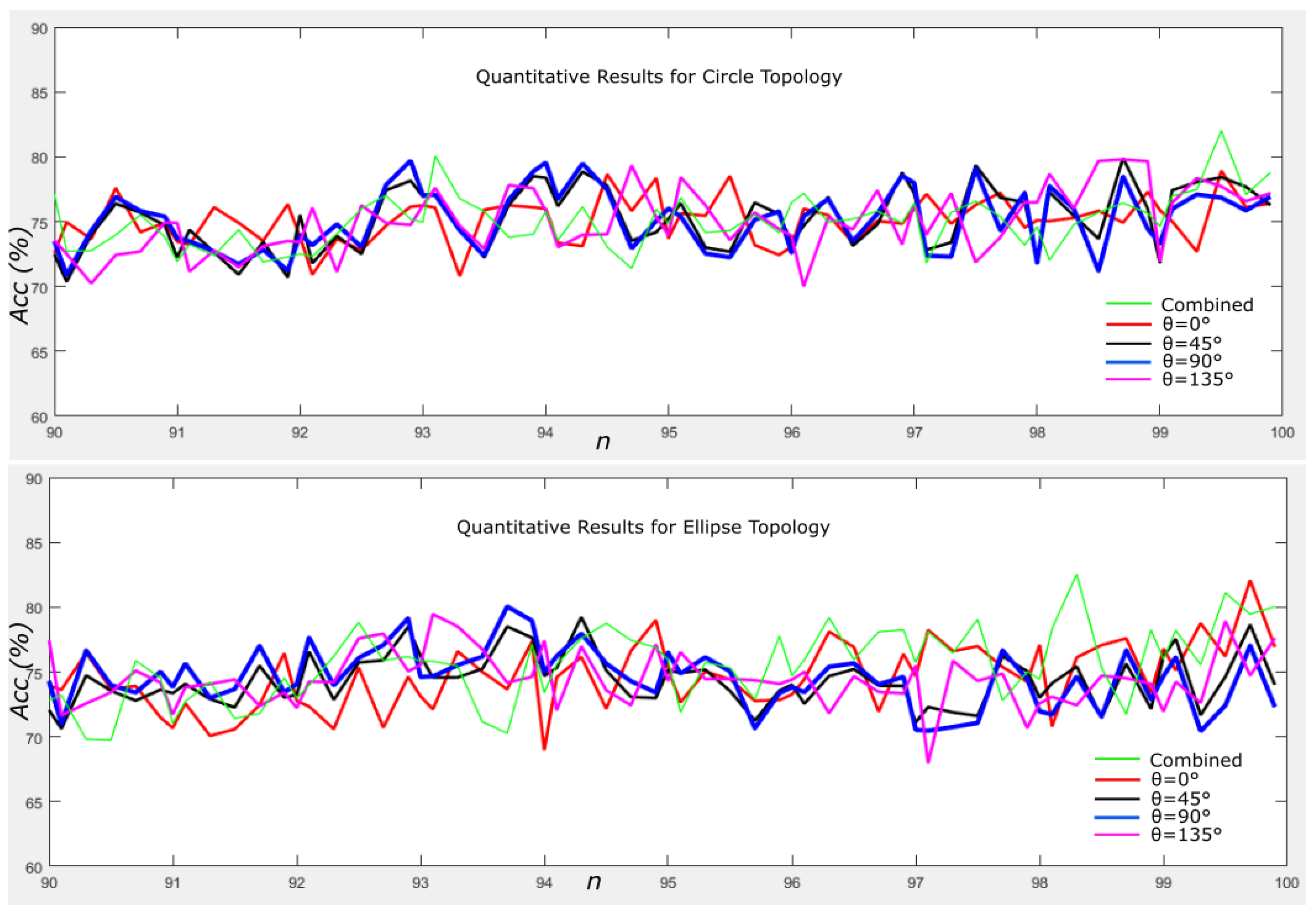
4.5. Results on Different Orientations
4.6. Summary of Quantitative Results
5. Discussion
5.1. Quantitative Comparisons
5.2. Effects of Parameter Selection
5.3. Future Work
6. Conclusions
Acknowledgments
Author Contributions
Conflicts of Interest
Abbreviations
| AUC | Area Under the Curve |
| BIF | Basic Image Features |
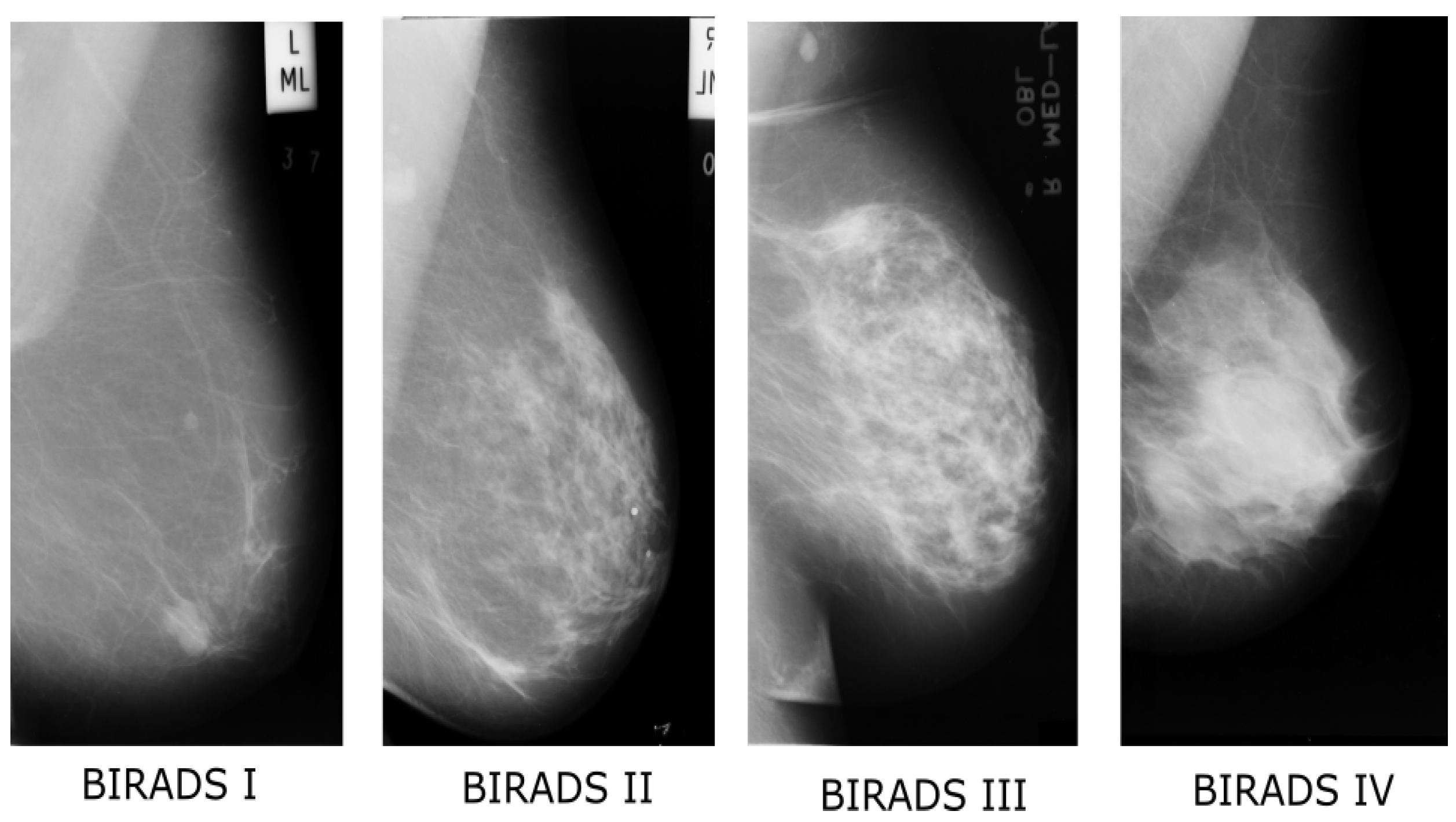
| BI-RADS | Breast Imaging-Reporting and Data System |
| CAD | Computer Aided Diagnosis |
| CNN | Convolutional Neural Network |
| FCM | Fuzzy C-means |
| LBP | Local Binary Pattern |
| LGA | Local Grey-level Appearance |
| LTP | Local Ternary Pattern |
| LQP | Local Quinary Pattern |
| MR8 | Maximum Response 8 filter bank |
| SFS | Sequential Forward Selection |
| SVM | Support Vector Machine |
| Fibro Glandular Region |
References
- Cancer Research UK. Breast cancer statistics. 2014. Available online: http://www.cancerresearchuk.org/health-professional/cancer-statistics/statistics-by-cancer-type/breast-cancer (accessed on 6 January 2017).
- Breast Cancer. U.S. Breast Cancer Statistics. 2016. Available online: http://www.breastcancer.org/symptoms/understand_bc/statistics (accessed on 6 January 2017).
- Oliver, A.; Freixenet, J.; Martí, R.; Pont, J.; Perez, E.; Denton, E.R.E.; Zwiggelaar, R. A Novel Breast Tissue Density Classification Methodology. IEEE Trans. Inf. Technol. Biomed. 2008, 12, 55–65. [Google Scholar] [CrossRef] [PubMed]
- Bovis, K.; Singh, S. Classification of Mammographic Breast Density Using a Combined Classifier Paradigm. In Proceedings of the 4th International Workshop on Digital Mammography, Nijmegen, Netherlands, 7–10 June 2002; pp. 177–180. [Google Scholar]
- Oliver, A.; Tortajada, M.; Lladó, X.; Freixenet, J.; Ganau, S.; Tortajada, L.; Vilagran, M.; Sentś, M.; Martí, R. Breast Density Analysis Using an Automatic Density Segmentation Algorithm. J. Digit. Imaging 2015, 28, 604–612. [Google Scholar] [CrossRef] [PubMed]
- Parthaláin, N.M.; Jensen, R.; Shen, Q.; Zwiggelaar, R. Fuzzy-rough approaches for mammographic risk analysis. Intell. Data Anal. 2010, 14, 225–244. [Google Scholar]
- Chen, Z.; Denton, E.; Zwiggelaar, R. Local feature based mamographic tissue pattern modelling and breast density classification. In Proceedings of the 4th International Conference on Biomedical Engineering and Informatics (BMEI), Shanghai, China, 15–17 October 2011; pp. 351–355. [Google Scholar]
- Bosch, A.; Munoz, X.; Oliver, A.; Martí, J. Modeling and Classifying Breast Tissue Density in Mammograms. In Proceedings of the IEEE Computer Society Conference on Computer Vision and Pattern Recognition (CVPR’06), New York, NY, USA, 17–22 June 2006; pp. 1552–1558. [Google Scholar]
- Chen, Z.; Oliver, A.; Denton, E.; Zwiggelaar, R. Automated Mammographic Risk Classification Based on Breast Density Estimation. In Pattern Recognition and Image Analysis; Volume 7887 of the series Lecture Notes in Computer Science; Springer: Berlin/Heidelberg, Germany, 2013; pp. 237–244. [Google Scholar]
- Wolfe, J.N. Risk for breast cancer development determined by mammographic parenchymal pattern. Cancer 1976, 37, 2486–2492. [Google Scholar] [CrossRef]
- He, W.; Denton, E.; Stafford, K.; Zwiggelaar, R. Mammographic Image Segmentation and Risk Classification Based on Mammographic Parenchymal Patterns and Geometric Moments. Biomed. Signal Process. Control 2011, 6, 321–329. [Google Scholar] [CrossRef]
- Petroudi, S.; Kadir, T.; Brady, M. Automatic Classification of Mammographic Parenchymal Patterns: A Statistical Approach. In Proceedings of the 25th Annual International Conference of the IEEE Engineering in Medicine and Biology Society (IEEE Cat. No.03CH37439), Cancun, Mexico, 17–21 September 2003; Volume 1, pp. 798–801. [Google Scholar]
- Keller, B.M.; Chen, J.; Daye, D.; Conant, E.F.; Kontos, D. Preliminary evaluation of the publicly available Laboratory for Breast Radiodensity Assessment (LIBRA) software tool: Comparison of fully automated area and volumetric density measures in a case-control study with digital mammography. Breast Cancer Res. 2015, 17, 1–17. [Google Scholar] [CrossRef] [PubMed]
- Rampun, A.; Morrow, P.J.; Scotney, B.W.; Winder, R.J. Breast density classification in mammograms using local quinary patterns. In Proceedings of the Annual Conference on Medical Image Understanding and Analysis MIUA 2017: Medical Image Understanding and Analysis, Edinburgh, UK, 11–13 July 2017; pp. 365–376. [Google Scholar]
- Moreira, I.C.; Amaral, I.; Domingues, I.; Cardoso, A.; Cardoso, M.J.; Cardoso, J.S. INbreast: Toward a full-field digital mammographic database. Acad. Radiol. 2011, 19, 236–428. [Google Scholar] [CrossRef] [PubMed]
- Byng, J.W.; Boyd, N.F.; Fishell, E.; Jong, R.A.; Yaffe, M.J. Automated analysis of mammographic densities. Phys. Med. Biol. 1996, 41, 909–923. [Google Scholar] [CrossRef] [PubMed]
- Muštra, M.; Grgić, M.; Delać, K. A Novel Breast Tissue Density Classification Methodology. Breast Density Classification Using Multiple Feature Selection. Automatika 2012, 53, 362–372. [Google Scholar]
- Suckling, J.; Parker, J.; Dance, D.; Astley, S.; Hutt, I.; Boggis, C.; Ricketts, I. The mammographic image analysis society digital mammogram database. Proc. Excerpta Med. Int. Congr. Ser. 1994, 375–378. [Google Scholar]
- Tamrakar, D.; Ahuja, K. Density-Wise Two Stage Mammogram Classification Using Texture Exploiting Descriptors. arXiv, 2017; arXiv:1701.04010. [Google Scholar]
- Ergin, S.; Kilinc, O. A new feature extraction framework based on wavelets for breast cancer diagnosis. Comput. Biol. Med. 2015, 51, 171–182. [Google Scholar] [CrossRef] [PubMed]
- Gedik, N. A new feature extraction method based on multiresolution representations of mammograms. Appl. Soft Comput. 2016, 44, 128–133. [Google Scholar] [CrossRef]
- Kooi, T.; Litjens, G.; van Ginnekena, B.; Gubern-Méridaa, A.; Sánchez, C.I.; Manna, R.; den Heeten, A.; Karssemeijer, N. Large scale deep learning for computer aided detection of mammographic lesions. Med. Image Anal. 2017, 35, 303–312. [Google Scholar] [CrossRef] [PubMed]
- Litjens, G.; Kooi, T.; Bejnordi, B.E.; Setio, A.A.A.; Ciompi, F.; Ghafoorian, M.; van der Laak, J.A.W.M.; van Ginneken, B.; Sánchez, C.I. A survey on deep learning in medical image analysis. Med. Image Anal. 2017, 42, 60–88. [Google Scholar] [CrossRef] [PubMed]
- Kallenberg, M.; Petersen, K.; Nielsen, M.; Ng, A.; Diao, P.; Igel, C.; Vachon, C.; Holland, K.; Karssemeijer, N.; Lillholm, M. Unsupervised deep learning applied to breast density segmentation and mammographic risk scoring. IEEE Trans. Med. Imaging 2016, 35, 1322–1331. [Google Scholar] [CrossRef] [PubMed]
- Ahn, C.K.; Heo, C.; Jin, H.; Kim, J.H. A Novel Deep Learning-based Approach to High Accuracy Breast Density Estimation in Digital Mammography. In Proceedings of the SPIE Medical Imaging 2017: Computer-Aided Diagnosis, Orlando, FL, USA, 3 March 2017; Volume 10134. [Google Scholar]
- Arevalo, J.; González, F.A.; Ramos-Pollán, R.; Oliveira, J.L.; Lopez, M.A.G. Representation learning for mammography mass lesion classification with convolutional neural networks. Comput. Methods Program. Biomed. 2016, 127, 248–257. [Google Scholar]
- Qiu, Y.; Wang, Y.; Yan, S.; Tan, M.; Cheng, S.; Liu, H.; Zheng, B. An initial investigation on developing a new method to predict short-term breast cancer risk based on deep learning technology. In Proceedings of the SPIE Medical Imaging 2016: Computer-Aided Diagnosis, San Diego, CA, USA, 24 March 2016; Volume 9785. [Google Scholar]
- Cheng, J.Z.; Ni, D.; Chou, Y.H.; Qin, J.; Tiu, C.M.; Chang, Y.C.; Huang, C.S.; Shen, D.; Chen, C.M. Computer-Aided Diagnosis with Deep Learning Architecture: Applications to Breast Lesions in US Images and Pulmonary Nodules in CT Scans. Sci. Rep. 2016, 15, 24454. [Google Scholar] [CrossRef] [PubMed]
- Jiao, Z.; Gao, X.; Wang, Y.; Li, J. A deep feature based framework for breast masses classification. Neurocomputing 2016, 197, 221–231. [Google Scholar] [CrossRef]
- Rampun, A.; Morrow, P.J.; Scotney, B.W.; Winder, R.J. Fully Automated Breast Boundary and Pectoral Muscle Segmentation in Mammograms. Artif. Intell. Med. 2017, 79, 28–41. [Google Scholar] [CrossRef] [PubMed]
- Ojala, T.; Pietikainen, M.; Maenpaa, T. Multiresolution gray-scale and rotation invariant texture classification with local binary patterns. IEEE Trans. Pattern Anal. Mach. Intell. 2002, 24, 971–987. [Google Scholar] [CrossRef]
- Hadid, A.; Pietikainen, M.K.; Zhao, G.; Ahonen, T. Computer Vision Using Local Binary Patterns; Springer: London, UK, 2011; pp. 13–47. [Google Scholar]
- Tan, X.; Triggs, B. Enhanced local texture feature sets for face recognition under difficult lighting conditions. In Analysis and Modelling of Faces and Gestures; Springer: Berlin/Heidelberg, Germany, 2007; pp. 168–182. [Google Scholar]
- Rampun, A.; Morrow, P.J.; Scotney, B.W.; Winder, J. A Quantitative Study of Local Ternary Patterns for Risk Assessment in Mammography. In Proceedings of the International Conference on Innovation in Medicine and Healthcare, Vilamoura, Portugal, 21–23 June 2017; pp. 283–286. [Google Scholar]
- Nanni, L.; Luminia, A.; Brahnam, S. Local binary patterns variants as texture descriptors for medical image analysis. Artif. Intell. Med. 2010, 49, 117–125. [Google Scholar] [CrossRef] [PubMed]
- Gio, Y.; Zhao, G.; Pietikäinen, M. Discriminative features for feature description. Pattern Recognit. 2012, 45, 3834–3843. [Google Scholar] [CrossRef]
- Rampun, A.; Wang, L.; Malcolm, P.; Zwiggelaar, R. A quantitative study of texture features across different window sizes in prostate t2-weighted mri. Procedia Comput. Sci. 2016, 90, 74–79. [Google Scholar] [CrossRef]
- Rampun, A.; Tiddeman, B.; Zwiggelaar, R.; Malcolm, P. Computer aided diagnosis of prostate cancer: A texton based approach. Med. Phys. 2016, 43, 5412–5425. [Google Scholar] [CrossRef] [PubMed]
- Rampun, A.; Zheng, L.; Malcolm, P.; Tiddeman, B.; Zwiggelaar, R. Computer-aided detection of prostate cancer in T2-weighted MRI within the peripheral zone. Phys. Med. Biol. 2016, 61, 4796–4825. [Google Scholar] [CrossRef] [PubMed]
- Rampun, A.; Morrow, P.J.; Scotney, B.W.; Winder, R.J. Breast density classification in mammograms using local ternary patterns. In Proceedings of the International Conference Image Analysis and Recognition ICIAR 2017: Image Analysis and Recognition, Montreal, QC, Canada, 5–7 July 2017; pp. 463–470. [Google Scholar]
- Aly, M. Survey on Multiclass Classification Methods. 2005. Available online: http://citeseerx.ist.psu.edu/viewdoc/summary?doi=10.1.1.175.107 (accessed on 4 December 2017).
- Landgrebe, T.C.W.; Duin, R.P.W. Approximating the multiclass ROC by pairwise analysis. Pattern Recognit. Lett. 2007, 28, 1747–1758. [Google Scholar] [CrossRef]


| Topologies | Equations | Parameters |
|---|---|---|
| Circle (ci) | R is the radius of the circle | |
| Ellipse (el) | a and b are the semimajor and semiminor axis lengths, where | |
| Parabola (par) | c is the distance between vertex and focus | |
| Hyperbola (hy) | a and b are the semimajor and semiminor axis lengths |
| Topologies | Multiresolution | Parameters |
|---|---|---|
| Circle | ||
| Ellipse | ||
| Parabola | ||
| Hyperbola | ||
| Topologies | Multiresolution | Parameters |
|---|---|---|
| Circle | ||
| Ellipse |
| Operators | Sen(%) | Spe(%) | Area Under the Curve(%) | Best n |
|---|---|---|---|---|
| 99.3 | ||||
| 97.6 | ||||
| 97.9 | ||||
| 98.5 | ||||
| 98.3 | ||||
| 93.7 | ||||
| 96.2 | ||||
| 99.2 | ||||
| 99.4 | ||||
| 93.7 |
| Oprators | Sen(%) | Spe(%) | AUC(%) | Best n |
|---|---|---|---|---|
| 99.5 | ||||
| 98.7 | ||||
| 92.9 | ||||
| 98.7 | ||||
| 94.5 | ||||
| 99.7 | ||||
| 94.3 | ||||
| 93.7 | ||||
| 93.1 | ||||
| 98.3 |
| Authors | Summary | Accuracy |
|---|---|---|
| Parthaláin et al. [6] | First and second-order statistical features and morphological features extracted from fatty and non-fatty tissues. The Fuzzy C-means (FCM) clustering approach was used to segment fatty and non-fatty tissues. Fuzzy-rough approaches were employed for feature selection and classification. The feature extraction pipeline is the same as the study of Oliver et al. [3]. | 91.4% |
| Our method | The Local Quinary Pattern (LQP) operators were used to extract local features within the fibro-glandular region using multiresolution and multi-orientation approaches. Only dominant patterns were used for classification using the support vector machine classifier. | 86.13% 82.02% |
| Oliver et al. [3] | First and second-order statistical features and morphological features extracted from fatty and non-fatty tissues. The Fuzzy C-means clustering approach was used to segment fatty and non-fatty tissues. This is the same as the study of Parthaláin et al. [3]. Several machine learning algorithms (e.g., k-Nearest Neighbours, decision tree and Bayes classifiers) were combined as a classification approach. | 86% |
| Rampun et al. [40] | The LTP operators were used to extract local features within the fibro-glandular region at different orientations. Feature from all orientations were concatenated to create a long feature vector. Subsequently, the support vector machine (SVM) classifier was employed in the testing phase. | 82.33% |
| Muštra et al. [17] | The first and second order statistical features were extracted at different orientations and resolutions. A combined paradigm of feature selection approach was employed to simplify complexity in the feature space. Finally, the k-Nearest Neighbours and Naive Bayesian classifiers were used to classify unseen cases. | 79.3% |
| Chen et al. [7,9] | Several texture descriptors based on the following feature extraction techniques were tested: the local binary pattern, local grey-level appearance, basic image features and Texton approaches. The k-NN classification approach was used to differentiate unseen cases into four BI-RADS classes. | 59–76% |
| Petroudi et al. [12] | The Maximum Response 8 (MR8) filter bank approach was used to extract the breast local information. Subsequently, the distribution was used to compare each of the resulting histograms from the training set to all the learned histogram models from the training set. | 75.5% |
| Bovis and Singh [4] | Texture features were extracted using Fourier and Discrete Wavelet transforms, and first and second-order statistical features. In the classification phase, a combined classifier paradigm (e.g., the SVM, Random Forest and k-NN) was used as a classification approach. | 71.4% |
| He et al. [4] | Class density was determined based on the relative proportions of the four Tabár building blocks within the whole breast region. | 70% |
© 2018 by the authors. Licensee MDPI, Basel, Switzerland. This article is an open access article distributed under the terms and conditions of the Creative Commons Attribution (CC BY) license (http://creativecommons.org/licenses/by/4.0/).
Share and Cite
Rampun, A.; Scotney, B.W.; Morrow, P.J.; Wang, H.; Winder, J. Breast Density Classification Using Local Quinary Patterns with Various Neighbourhood Topologies. J. Imaging 2018, 4, 14. https://doi.org/10.3390/jimaging4010014
Rampun A, Scotney BW, Morrow PJ, Wang H, Winder J. Breast Density Classification Using Local Quinary Patterns with Various Neighbourhood Topologies. Journal of Imaging. 2018; 4(1):14. https://doi.org/10.3390/jimaging4010014
Chicago/Turabian StyleRampun, Andrik, Bryan William Scotney, Philip John Morrow, Hui Wang, and John Winder. 2018. "Breast Density Classification Using Local Quinary Patterns with Various Neighbourhood Topologies" Journal of Imaging 4, no. 1: 14. https://doi.org/10.3390/jimaging4010014
APA StyleRampun, A., Scotney, B. W., Morrow, P. J., Wang, H., & Winder, J. (2018). Breast Density Classification Using Local Quinary Patterns with Various Neighbourhood Topologies. Journal of Imaging, 4(1), 14. https://doi.org/10.3390/jimaging4010014