A Parametric LFP Battery Degradation Model for Techno-Economic Assessment of European System-Imbalance Services

Abstract

Battery energy storage systems (BESSs) are increasingly deployed by European Balance Responsible Parties (BRPs) to mitigate system-imbalance exposure; yet, techno-economic assessments often represent degradation using fixed-lifetime or equivalent-full-cycle assumptions that obscure the dependence of wear on operating policy and sizing. This study develops a data-driven, parameterised degradation framework for LiFePO₄ (LFP) BESS operating under imbalance duty. Using historical imbalance datasets from five European countries spanning eight transmission system operators (TSOs), annual cycle-induced capacity loss, calendar-induced capacity loss, and total annual capacity loss at 25 °C are mapped as explicit functions of energy-to-power ratio (duration), maximum power rating, depth of discharge, state-of-charge operating bounds, and daily cycling intensity. A degree-2 Ridge specification yields compact, auditable coefficients that transfer across entities (including an out-of-time full-year hold-out for Belgium, 2025). The fitted response surfaces reveal consistent EU-wide operating regimes: cycling-dominant ageing for durations $\le 3$ h, a mixed regime for durations $\approx 3$–6 h, and calendar-dominant ageing for durations $\ge 6$ h, indicating a practical compromise around ≈4–5.5 h. The resulting coefficientised outputs are Techno-Economic Assessment (TEA)-ready and enable risk-aware sizing and state-of-charge policy design for imbalance-focused BESS portfolios.

1. Introduction

1.1. Background

Grid-connected battery energy storage systems (BESSs) are increasingly deployed to manage system imbalance across European transmission networks. In total, 4.9 GW of utility-scale storage was added in 2024, bringing the cumulative EU total above 13 GW [1]. In the European system-imbalance operation, Balancing Responsible Parties (BRPs) are financially responsible for deviations between nominated and realised volumes and may deploy BESS to hedge forecast-error risk. These obligations shape operating patterns, from high-SOC availability to frequent shallow cycling [2,3,4]. Lithium iron phosphate (LFP) is widely adopted for stationary use because of its safety, benign thermal behaviour, and strong cycle life [5]. Battery lifetime depends on both calendar and cycle ageing and is sensitive to temperature and state of charge (SOC), motivating models that represent both mechanisms [6,7].

Consequently, battery lifetime outcomes depend on prequalified grid power ($P_{max}$), the energy-to-power ratio ($E/P$, i.e., duration), the SOC window (upper and lower bounds), depth of discharge (DoD), daily cycling frequency, and temperature. A tractable annualised degradation representation that captures these drivers is needed to inform realistic techno-economic assessments and to guide dispatch and sizing for grid services [8].

Existing lifetime treatments in grid-facing models are often (i) application-agnostic linear throughput costs or fixed replacement schedules; (ii) cycle-only formulations that ignore calendar ageing and high-SOC standby; or (iii) high-fidelity electrochemical models that are too complex for long-horizon planning. Such choices can distort operational decisions and profitability: when degradation is ignored, or mis-specified, ex-post wear costs can overturn seemingly profitable trades, whereas including realistic degradation alters optimal dispatch and improves lifetime economics [9,10,11].

Several studies have explored parametrised ageing models for lithium-ion batteries, although relatively few have been developed in a form that is directly embeddable in techno-economic assessment and dispatch optimisation. Sui et al. conducted a long-term calendar-ageing study on commercial LiFePO₄/graphite cells and fitted degradation parameters across temperature and SOC conditions using a two-step nonlinear regression approach, highlighting the coupled influence of thermal and SOC stressors on capacity fade [12]. Complementary contributions by Birkl and Howey, and later co-workers, used current-pulse testing and electrochemical impedance spectroscopy (EIS) with identification/fitting procedures to estimate dynamic and impedance-model parameters relevant to state-of-health tracking, with an emphasis on dynamic behaviour rather than annualised ageing response surfaces for system-level optimisation [13,14]. More broadly, O’Kane et al. reviewed mechanistic and semi-empirical degradation models and emphasised the practical difficulty of coupling multiple degradation pathways without extensive experimental datasets for parameterisation [15]. While these works demonstrate mature parameter identification and degradation modelling foundations, they typically do not provide reduced-form ageing representations tailored to techno-economic scheduling. Recent work has begun to embed ageing-aware operation directly into profit optimisation of battery energy storage systems, explicitly trading operational revenue against degradation-induced lifetime costs [16]. In this context, the remaining gap was addressed in this work by integrating a semi-empirical LFP ageing formulation within an end-to-end techno-economic framework and by providing auditable regression coefficients that map dispatch-relevant stressors (e.g., energy-to-power ratio, SOC limits, and cycling intensity) to annualised cycle- and calendar-induced capacity loss. In the absence of such a model, techno-economic results can be biassed, and dispatch, sizing, and availability decisions may be systematically suboptimal, particularly under imbalance settlement, thereby constituting a critical gap addressed in this paper. Moreso, directly comparable studies at the intersection of (i) European system-imbalance operation, (ii) scenario-level parameter sweeps, and (iii) coefficientised LFP degradation response surfaces remain scarce. Accordingly, there is a clear need for simplified yet robust degradation models suitable for annual and lifecycle economic analyses of grid-scale storage.

1.2. Study Aim

This study develops and validates a simplified, parameterised, and robust annual degradation framework for LFP batteries operating in European system-imbalance services. The framework quantifies calendar ($Q_{\mathrm{cal}}$), cyclic ($Q_{\mathrm{cyc}}$), and total ($Q_{\mathrm{tot}}$) capacity loss as explicit functions of grid and battery parameters. It is intended to enable regulators to set realistic minimum requirements and lifetime-aware performance metrics; system operators to design dispatch and availability policies that avoid unintended calendar-dominant wear; and project developers to select $P_{max}$, $E/P$, SOC limits, and DoD policies that jointly optimise profitability, compliance, and asset longevity. The resulting improvements in realism strengthen bankability assessments and reduce the risk of early capacity shortfalls.

1.3. Contribution to Knowledge

To the best of our knowledge, this paper provides the first data-driven, parameterised, and operationally interpretable LFP degradation framework explicitly tailored to the management of European system-imbalance portfolios by BRPs. Addressing a critical gap wherein investment planning has typically assumed fixed lifetimes or equivalent-full-cycle (EFC) heuristics, the study learns from historical imbalance data to produce annual $Q_{\mathrm{cyc}}$, $Q_{\mathrm{cal}}$, and $Q_{\mathrm{tot}}$ at 25 °C as explicit functions of $E/P$, $P_{max}$, DoD, $SO{C}_{min}$/$SO{C}_{max}$, and daily cycling intensity. The coefficientised Ridge formulation is compact and auditable, enabling risk-averse techno-economic assessment and dispatch optimisation that internalises degradation rather than assuming it, which is highly pertinent for BRPs mitigating forecast-error exposure in imbalance settlement.

Beyond accuracy and cross-entity validation (nine major European entities, including an external hold-out), the framework contributes a regime map that quantifies when $Q_{\mathrm{tot}}$ is cycle- versus calendar-dominated and shows how $E/P$, $P_{max}$, and DoD shift that boundary. The model thereby identifies actionable levers, notably SOC-window policy and sizing ($E/P$), to balance utilisation and longevity in merchant operation. Overall, the work replaces assumption-based degradation practice with calibrated, TEA-ready parametric surfaces for system-imbalance duty, establishing a transferable basis for portfolio optimisation, investment appraisal, and risk management across European TSOs.

2. Methodology

2.1. Data Collection and Case-Study Overview

To capture a diverse range of European balancing conditions, five countries were selected, each with historical imbalance price and volume data: Belgium, the Netherlands, Germany (reported per TSO control zone), Spain, and Poland. The study covers Belgium (Elia, 2020–2025), the Netherlands (TenneT NL, 2020–2023), Germany—50 Hertz (2022–2025), Germany—Amprion (2022–2025), Germany—TenneT DE (2022–2025), Germany—TransnetBW (2022–2025), Spain (REE, 2022–2025), and Poland (PSE, 2022–2025).

Historical imbalance price and volume data for Belgium were obtained from Elia’s Open Data platform [17,18,19], while the Netherlands data were obtained directly from TenneT NL [20]. For Germany, Spain, and Poland, the datasets were sourced from the ENTSO-E Transparency Platform [21]. All time series were aligned to utc, cleaned for missing or duplicate timestamps to ensure comparability across regions and years. The resulting dataset forms a multi-year, high-resolution record of imbalance conditions across eight European balancing zones, reflecting a wide range of grid dynamics and operational behaviours. Table 1 summarises the global scenarios used in the simulations.

Table 1. Global scenario grid applied in each zone/year.

Parameter	Units	Values	Notes
Strategy	—	Naïve	Always counteracts imbalance; no price-based arbitrage.
Power sweep	MW	$P_{max}\in \{50,100,\dots ,600\}$	Step = 50 MW (12 values).
Duration sweep	h	$E/P\in \{0.5,1,2,4,6,8,10\}$	Seven duration settings.
SOC windows	—	(0.50–0.50, 0.00), (0.45–0.55, 0.10), (0.40–0.60, 0.20), (0.35–0.65, 0.30), (0.30–0.70, 0.40), (0.25–0.75, 0.50), (0.20–0.80, 0.60), (0.15–0.85, 0.70), (0.10–0.90, 0.80), (0.05–0.95, 0.90), (0.00–1.00, 1.00)	Paired ${\mathrm{SOC}}_{min}$–${\mathrm{SOC}}_{max}$ (per-unit), with corresponding $\mathrm{DoD}$ (per-unit).
DoD windows	—	$\{0.0,0.1,\dots ,1.0\}$	$\mathrm{DoD}={\mathrm{SOC}}_{max}-{\mathrm{SOC}}_{min}$.
Ambient temp.	°C	25	Used in calendar-ageing factors.
Time step	min	1	Data up-sampled from ISP to 1 min for integration.
Initial SOC	—	0.50	Mid-point start.

2.2. Battery Simulation Framework

An end-to-end, scenario-based simulation workflow was implemented to translate historical system-imbalance conditions into annual LFP BESS degradation indicators, as summarised in Figure 1. For each entity/year, the framework ingests system-imbalance time series (imbalance volumes and, where applicable, imbalance prices), applies harmonisation and minute-resolution resampling, and evaluates a structured scenario grid spanning power rating $P_{max}$, duration ($E/P$), and SOC-window policies $(SO{C}_{min},SO{C}_{max})$ (hence DoD). For each scenario, a physics-informed BESS operational simulation produces minute-level dispatch and SOC trajectories, including a converter/round-trip efficiency representation and an imbalance-mitigation control strategy. Cycling stress metrics are subsequently derived from the SOC trajectory using half-cycle detection (rainflow-equivalent), yielding DoC-, C-rate-, and full-equivalent-cycle (FEC) sequences. These stress metrics parameterise the semi-empirical Naumann et al. LiFePO₄/graphite ageing model, which is accumulated in discrete time to produce scenario-level annual capacity-loss outputs $Q_{\mathrm{cyc}}$, $Q_{\mathrm{cal}}$, and $Q_{\mathrm{tot}}$. Aggregating results across all scenarios/entities/years yields the regression dataset used to estimate compact degree-2 parametric response surfaces for $Q_{\mathrm{cyc}}$ and $Q_{\mathrm{tot}}$ (with $Q_{\mathrm{cal}}=Q_{\mathrm{tot}}-Q_{\mathrm{cyc}}$), validated via within-entity splits and an external full hold-out (BE/2025). Unless otherwise stated, simulations assume a fixed ambient temperature of 25 °C and an initial SOC of 50%, consistent with controlled utility-scale container operation.

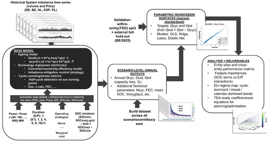
Figure 1. End-to-end framework: Historical system-imbalance datasets define scenario grids and drive minute-resolution BESS dispatch; cycle counting and Naumann-based ageing accumulation yield scenario-level annual losses ($Q_{\mathrm{cyc}}$, $Q_{\mathrm{cal}}$, $Q_{\mathrm{tot}}$), which are then used to fit and validate degree-2 parametric regression surfaces and derive TEA-ready deliverables.

2.2.1. SOC Dynamics and Power Constraints

At discrete minute index t (time step $\Delta t=1\min$), the system imbalance $\mathrm{SI}\left(t\right)$ (MW; positive for surplus, negative for deficit) is mapped to battery power $P_{\mathrm{bat}}\left(t\right)$ (MW; positive for charging, negative for discharging) subject to the converter power limit $P_{max}$ (MW):

$$P_{\mathrm{bat}}\left(t\right)=\left\{\begin{array}{cc}min\{\mathrm{SI}\left(t\right),P_{max}\},\hfill & \mathrm{SI}\left(t\right)>0\left(\mathrm{charge}\right),\hfill \\ max\{-P_{max},\mathrm{SI}\left(t\right)\},\hfill & \mathrm{SI}\left(t\right)<0\left(\mathrm{discharge}\right),\hfill \\ 0,\hfill & \mathrm{SI}\left(t\right)=0,\hfill \end{array}\right.\mathrm{with}\left|P_{\mathrm{bat}}\left(t\right)\right|\le P_{max}.$$

(1)

The state of charge, $\mathrm{SOC}\left(t\right)$, is represented on a normalised scale $[0,1]$ and is advanced each step and bounded to $[{\mathrm{SOC}}_{min},{\mathrm{SOC}}_{max}]$ (both dimensionless):

$$\mathrm{SOC}(t+\Delta t)=\mathrm{SOC}\left(t\right)+{\displaystyle \frac{P_{\mathrm{bat}}\left(t\right)(\Delta t/60)}{E_{\mathrm{bat}}}},$$

(2)

where $E_{\mathrm{bat}}$ is the usable energy capacity (MWh) over the $0–100\%$ SOC range and $\Delta t/60$ converts minutes to hours. For each scenario, the energy capacity is linked to sizing via $E_{\mathrm{bat}}=(E/P)P_{max}$, with $E/P$ expressed in hours. Requests that would breach SOC limits are curtailed; residual imbalance beyond BESS limits is recorded.

2.2.2. Converter Efficiency Model

Round-trip efficiency depends on the instantaneous converter loading $p=100|P_{\mathrm{bat}}\left(t\right)|/P_{max}$ (dimensionless, in %), where $|P_{\mathrm{bat}}\left(t\right)|$ is the absolute battery power and $P_{max}$ is the rated power (MW). A fitted curve ${\eta }_{\mathrm{rt}}\left(p\right)$ (dimensionless fraction in $[0,1]$) represents inverter and internal losses. The round-trip efficiency curve was parameterised from Schimpe et al.’s utility-scale measurements (cell and inverter), then compactly re-fit for the dispatcher [22].

$${\eta }_{\mathrm{rt}}\left(p\right)={\displaystyle \frac{-6.7843\times {10}^{-4}{p}^2+0.02723p+90.983-34.796e^{-0.162p}}{100}},0\le p\le 100,$$

(3)

where e denotes the base of the natural logarithm. Efficiency is applied to energy flows (i.e., the delivered/withdrawn energy associated with $P_{\mathrm{bat}}\left(t\right)$ is adjusted by ${\eta }_{\mathrm{rt}}\left(p\right)$); dispatch remains imbalance-driven.

2.2.3. Degradation Modelling

Total degradation is represented as the superposition of calendar- and cycle-induced ageing contributions for both capacity fade and resistance growth. The functional forms follow the semi-empirical LiFePO₄/graphite ageing model of Naumann et al. [23,24]. The formulation is evaluated in discrete time and annualised at a fixed ambient temperature of 25 °C for the SOC/DoD grids considered in this work.

Calendar-induced capacity fade and resistance growth are expressed as

$$\begin{array}{cccc}\hfill Q_{\mathrm{cal}}(t,s)& =k_T^Q{k}_{\mathrm{SOC}}^Q\left(s\right)\sqrt{t},\hfill & \hfill R_{\mathrm{cal}}(t,s)& =k_T^R{k}_{\mathrm{SOC}}^R\left(s\right)t,\hfill \end{array}$$

(4)

where $Q_{\mathrm{cal}}$ is calendar capacity loss (%), $R_{\mathrm{cal}}$ is calendar resistance growth (%), t is elapsed time (h), and s is the state of charge (SOC; fraction in $[0,1]$). The factors $k_T^Q$ and $k_T^R$ are temperature-dependent rate terms, while $k_{\mathrm{SOC}}^Q\left(s\right)$ and $k_{\mathrm{SOC}}^R\left(s\right)$ are dimensionless SOC modifier functions.

The temperature factors $k_T^Q$ and $k_T^R$ follow Arrhenius scaling:

$$k_T=k_{\mathrm{ref}}exp\left[-{\displaystyle \frac{E_A}{R_g}}\left({\displaystyle \frac{1}{T}}-{\displaystyle \frac{1}{T_{\mathrm{ref}}}}\right)\right],T_{\mathrm{ref}}=298.15\mathrm{K},T=25+273.15\mathrm{K},$$

(5)

where $k_{\mathrm{ref}}$ is the reference rate constant, $E_A$ is the activation energy (J mol⁻¹), $R_g$ is the universal gas constant (J mol⁻¹ K⁻¹), T is the temperature (K), and $T_{\mathrm{ref}}$ is the reference temperature (K). SOC sensitivity is captured via the modifiers

$$\begin{array}{cc}\hfill k_{\mathrm{SOC}}^Q\left(s\right)& =2.8575{(s-0.5)}^3+0.60225,\hfill \end{array}$$

(6)

$$\begin{array}{cc}\hfill k_{\mathrm{SOC}}^R\left(s\right)& =-3.3903{(s-0.5)}^2+1.5604.\hfill \end{array}$$

(7)

These terms impose a higher calendar-ageing rate at elevated SOC, consistent with the underlying empirical calibration reported in [23].

Cycle-induced capacity fade and resistance growth are expressed as

$$\begin{array}{cccc}\hfill Q_{\mathrm{cyc}}(F,c,d)& =k_c^Q\left(c\right)k_d^Q\left(d\right)\sqrt{F},\hfill & \hfill R_{\mathrm{cyc}}(F,c,d)& =k_c^R\left(c\right)k_d^R\left(d\right)F,\hfill \end{array}$$

(8)

where $Q_{\mathrm{cyc}}$ is cyclic capacity loss (%), $R_{\mathrm{cyc}}$ is cyclic resistance growth (%), F is cumulative full-equivalent cycles (FEC; dimensionless), c is the effective C-rate, and d is depth-of-cycle (DoC; fraction in $[0,1]$). The functions $k_c^Q\left(c\right)$ and $k_c^R\left(c\right)$ are dimensionless C-rate modifiers, and $k_d^Q\left(d\right)$ and $k_d^R\left(d\right)$ are dimensionless DoC modifiers. The cycle modifiers are given by

$$\begin{array}{cccc}\hfill k_c^Q\left(c\right)& =0.0630c+0.0971,\hfill & \hfill k_c^R\left(c\right)& =-0.0020c+0.0021,\hfill \end{array}$$

(9)

$$\begin{array}{cccc}\hfill k_d^Q\left(d\right)& =4.0253{(d-0.6)}^3+1.0923,\hfill & \hfill k_d^R\left(d\right)& =6.8477{(d-0.5)}^3+0.91882,\hfill \end{array}$$

(10)

which encode the empirical sensitivities to effective C-rate and cycle depth described in [24]. The square-root dependence of capacity fade on F, and the linear dependence of resistance growth on F, are retained from the original model structure.

The quantities F, c, and d are obtained from the simulated SOC trajectory via half-cycle detection (rainflow-equivalent turning-point identification). For each detected half-cycle, the corresponding DoC and an effective C-rate are computed from the associated SOC excursion and power trajectory, and cumulative FEC is updated accordingly. This procedure yields stepwise increments in F consistent with the occurrence and depth of cycling throughout the imbalance-following operation.

All simulations are performed at 1 min resolution. Let step i have duration $\Delta t$ (h), time $t_i$, SOC $s_i$, and cumulative FEC $F_i$. Calendar increments are accumulated using the following incremental square-root (for $Q_{\mathrm{cal}}$) and linear-time (for $R_{\mathrm{cal}}$) forms:

$$\begin{array}{cccc}\hfill \Delta Q_{\mathrm{cal},i}& =k_T^Q{k}_{\mathrm{SOC}}^Q\left(s_i\right)\left(\sqrt{t_i}-\sqrt{t_{i-1}}\right),\hfill & \hfill \Delta R_{\mathrm{cal},i}& =k_T^R{k}_{\mathrm{SOC}}^R\left(s_i\right)\Delta t.\hfill \end{array}$$

(11)

Cycle increments are evaluated only when F increases between steps (i.e., when cycling is detected), using

$$\begin{array}{cccc}\hfill \Delta Q_{\mathrm{cyc},i}& =k_c^Q\left(c_i\right)k_d^Q\left(d_i\right)\left(\sqrt{F_i}-\sqrt{F_{i-1}}\right),\hfill & \hfill \Delta R_{\mathrm{cyc},i}& =k_c^R\left(c_i\right)k_d^R\left(d_i\right)\left(F_i-F_{i-1}\right),\hfill \end{array}$$

(12)

where $c_i$ and $d_i$ denote the effective C-rate and DoC associated with the detected cycle contribution at step i.

Annual quantities are obtained by summing increments over the full year, yielding $Q_{\mathrm{cal}}$, $Q_{\mathrm{cyc}}$, $R_{\mathrm{cal}}$, and $R_{\mathrm{cyc}}$. Total degradation is then

$$Q_{\mathrm{tot}}=Q_{\mathrm{cal}}+Q_{\mathrm{cyc}},R_{\mathrm{tot}}=R_{\mathrm{cal}}+R_{\mathrm{cyc}},$$

(13)

where $Q_{\mathrm{tot}}$ and $R_{\mathrm{tot}}$ denote total annual capacity loss (%) and total annual resistance growth (%), respectively. The present work focuses on annual capacity loss $(Q_{\mathrm{cal}},Q_{\mathrm{cyc}},Q_{\mathrm{tot}})$ as the degradation outputs used for subsequent regression and techno-economic assessment.

2.2.4. Energy Management Strategy

An imbalance-following control rule is applied at each simulation step to mitigate the realised system imbalance. A requested battery power set-point is formed directly from the imbalance signal: the BESS charges for $\mathrm{SI}\left(t\right)>0$ (surplus) and discharges for $\mathrm{SI}\left(t\right)<0$ (deficit). The request is then enforced subject to the power constraint $|P_{\mathrm{bat}}\left(t\right)|\le P_{max}$ and the SOC operating window $[{\mathrm{SOC}}_{min},{\mathrm{SOC}}_{max}]$, with any infeasible portion curtailed and recorded as residual imbalance (see Equations (1) and (2)). Converter losses are represented via the load-dependent round-trip efficiency model in Equation (3), which is applied to energy flows (SOC evolution) while the dispatch decision remains imbalance-driven. No speculative price arbitrage is performed. Results, therefore, correspond to an ex-post replay of historical imbalance conditions at 1 min resolution.

Although the scenario dataset is generated using this imbalance-following dispatch, the fitted regression model is formulated in terms of operating stress descriptors $(E/P,P_{max},N_{\mathrm{cyc}},\mathrm{DoD},{\mathrm{SOC}}_{min},{\mathrm{SOC}}_{max})$ rather than dispatch logic. Consequently, alternative dispatch strategies (e.g., price-optimised or co-optimised policies) may be evaluated by computing the same descriptors from the realised annual operation and applying the coefficientised model obtained in this work.

2.3. Model Development and Parameterization

A regression modelling framework was constructed using the scenario-level dataset generated by the simulation and degradation workflow described in the preceding section. Each scenario corresponds to one entity/year and one operating-policy realisation on the parameter grid (power rating, duration, SOC window, and resulting cycling statistics). For each scenario, the simulation produces internally consistent annual degradation labels and summary operating descriptors, which are then used to fit compact parametric response surfaces for techno-economic assessment.

2.3.1. Targets

The cyclic and total annual capacity-loss components, $Q_{\mathrm{cyc}}$ and $Q_{\mathrm{tot}}$ (in % per year), are modelled directly. The calendar component is reconstructed as a residual:

$$Q_{\mathrm{tot}}=Q_{\mathrm{cyc}}+Q_{\mathrm{cal}}\Rightarrow Q_{\mathrm{cal}}=Q_{\mathrm{tot}}-Q_{\mathrm{cyc}},$$

(14)

consistent with the additive decomposition of capacity fade in the underlying semi-empirical Naumann et al. ageing formulation and with the simulation outputs, in which $Q_{\mathrm{cal}}$, $Q_{\mathrm{cyc}}$, and $Q_{\mathrm{tot}}$ are computed coherently from the same SOC trajectory. This choice enforces the physical additivity constraint at the regression stage and avoids redundancy that can arise when fitting three separate response surfaces. Because ${\widehat{Q}}_{\mathrm{cal}}$ is obtained by differencing two predictions, its uncertainty reflects the combined prediction errors of ${\widehat{Q}}_{\mathrm{tot}}$ and ${\widehat{Q}}_{\mathrm{cyc}}$; therefore, robustness of the inferred calendar component is supported by the out-of-sample performance of both fitted models (including the external full-year hold-out).

2.3.2. Predictors

For each scenario, the predictor vector $\mathbf{x}\in {\mathbb{R}}^6$ collects the configuration and operating descriptors

$$\mathbf{x}=\left[\begin{array}{c}{x}_1\\ x_2\\ x_3\\ x_4\\ x_5\\ x_6\end{array}\right]=\left[\begin{array}{c}E/P\\ P_{max}\\ N_{\mathrm{cyc}}\\ \mathrm{DoD}\\ {\mathrm{SOC}}_{min}\\ {\mathrm{SOC}}_{max}\end{array}\right],$$

(15)

where $E/P$ is the energy-to-power ratio (h), $P_{max}$ is the rated power (MW), $N_{\mathrm{cyc}}$ is the average cycles-per-day metric derived from the simulated SOC trajectory, $\mathrm{DoD}={\mathrm{SOC}}_{max}-{\mathrm{SOC}}_{min}$ is the depth of discharge, and ${\mathrm{SOC}}_{min},{\mathrm{SOC}}_{max}$ are the lower/upper SOC bounds.

2.3.3. Standardisation and Polynomial Basis

All predictors are z-scored using the training split statistics, i.e., $x_k\leftarrow (x_k-{\mu }_k)/{\sigma }_k$. Polynomial degrees 1–4 were evaluated; degree 2 provided the best balance between complexity, accuracy, and cross-entity transfer.

2.3.4. Quadratic Model

For each target $Q\in \{Q_{\mathrm{cyc}},Q_{\mathrm{tot}}\}$, the degree-2 model is written compactly as

$$\widehat{Q}=a_0+{\mathsf{\beta }}^{\top }\mathbf{x}+{\mathbf{x}}^{\top }\mathbf{H}\mathbf{x},$$

(16)

where $a_0\in \mathbb{R}$ is the intercept, $\mathsf{\beta }\in {\mathbb{R}}^6$ contains linear coefficients, and $\mathbf{H}\in {\mathbb{R}}^{6\times 6}$ is a symmetric matrix capturing quadratic and pairwise interaction effects.

Expanding Equation (16) yields

$$\widehat{Q}=a_0+\sum _{i=1}^6{\beta }_i{x}_i+\sum _{i=1}^6{\gamma }_{ii}{x}_i^2+\sum _{1\le i<j\le 6}{\gamma }_{ij}{x}_i{x}_j,$$

(17)

where ${\gamma }_{ii}$ are quadratic coefficients and ${\gamma }_{ij}$ are interaction coefficients. The mapping to the matrix form is $H_{ii}={\gamma }_{ii}$ and $H_{ij}=H_{ji}={\gamma }_{ij}/2$, so that ${\mathbf{x}}^{\top }\mathbf{H}\mathbf{x}$ produces each interaction term $x_i{x}_j$ once (no double counting).

For each target, the training split contains n scenario observations, collected in the response vector $\mathbf{y}\in {\mathbb{R}}^n$. The corresponding polynomial feature expansion is assembled in the design matrix $\mathsf{\Phi }\in {\mathbb{R}}^{n\times p}$ by concatenating an intercept column, the standardised predictors, their elementwise squares, and all unique pairwise interactions:

$$\mathsf{\Phi }=\left[\mathbf{1}\left|\mathbf{X}\right|{\mathbf{X}}^{\odot 2}|{\left\{x_i{x}_j\right\}}_{i<j}\right],\mathsf{\theta }=\left[a_0;\mathsf{\beta };\left\{{\gamma }_{ii}\right\};\left\{{\gamma }_{ij}\right\}\right],$$

(18)

where $\mathbf{X}\in {\mathbb{R}}^{n\times 6}$ stacks the standardised predictor vectors row-wise, ${\mathbf{X}}^{\odot 2}$ denotes elementwise squaring, and ${\left\{x_i{x}_j\right\}}_{i<j}$ denotes the set of all unique pairwise products. The parameter vector $\mathsf{\theta }\in {\mathbb{R}}^p$ collects the associated intercept, linear, quadratic, and interaction coefficients.

Model parameters are obtained by penalised least squares:

$$\widehat{\mathsf{\theta }}=arg\underset{\mathsf{\theta }}{min}{∥\mathbf{y}-\mathsf{\Phi }\mathsf{\theta }∥}_2^2+\mathcal{P}\left(\mathsf{\theta }\right),$$

(19)

with the intercept left unpenalised; ${\mathsf{\theta }}_{-0}$ denotes $\mathsf{\theta }$ with $a_0$ removed.

2.3.5. Regularised Estimators

The penalty term $\mathcal{P}\left(·\right)$ defines the estimator:

$$\begin{array}{cc}\hfill \mathrm{OLS}:& \mathcal{P}\left(\mathsf{\theta }\right)=0,\hfill \end{array}$$

(20)

$$\begin{array}{cc}\hfill \mathrm{Ridge}:& \mathcal{P}\left(\mathsf{\theta }\right)=\alpha {∥{\mathsf{\theta }}_{-0}∥}_2^2,\alpha ={10}^{-3},\hfill \end{array}$$

(21)

$$\begin{array}{cc}\hfill \mathrm{Lasso}:& \mathcal{P}\left(\mathsf{\theta }\right)=\alpha {∥{\mathsf{\theta }}_{-0}∥}_1,\alpha =0.1,\hfill \end{array}$$

(22)

$$\begin{array}{cc}\hfill \mathrm{Elastic}\mathrm{Net}:& \mathcal{P}\left(\mathsf{\theta }\right)=\alpha \left[\lambda {∥{\mathsf{\theta }}_{-0}∥}_1+(1-\lambda ){∥{\mathsf{\theta }}_{-0}∥}_2^2\right],\alpha =0.1,\lambda =0.5.\hfill \end{array}$$

(23)

Models are fitted separately for $Q_{\mathrm{cyc}}$ and $Q_{\mathrm{tot}}$; $Q_{\mathrm{cal}}$ is subsequently computed using Equation (14).

2.4. Training and Validation

The regression dataset was partitioned on a per-entity basis using an 80/20 random split across scenarios. Here, each observation corresponds to a complete, annualised simulation outcome for a unique operating scenario (i.e., a specific combination of $E/P$, $P_{max}$, $(SO{C}_{min},SO{C}_{max})$ and the associated cycling descriptors), rather than minute-level time-series samples. The split, therefore, separates operating scenarios within each entity and avoids temporal leakage at the time-step level. In addition to the within-entity scenario split, an external out-of-sample test was performed by holding out an entire year of data (Belgium 2025) from training and using it exclusively for testing.

All input variables were standardised, and a second-degree polynomial expansion was applied consistently across models. Each regression model was trained separately for $Q_{\mathrm{tot}}$ and $Q_{\mathrm{cyc}}$, after which $Q_{\mathrm{cal}}$ was reconstructed by difference. Model performance was evaluated using the coefficient of determination ($R^2$), mean absolute error (MAE), and root mean squared error (RMSE).

Comparative assessments across model types and polynomial degrees indicated that degree-2 polynomial models with the specified regularisation parameters achieved the most accurate and robust predictions across all test cases. These configurations were, therefore, selected as the final models for subsequent degradation prediction and feature-importance analysis.

3. Results and Discussion

3.1. Comparative Models: OLS, Lasso, Ridge, and Elastic Net

Table 2 summarises the cross-entity test performance of OLS, Ridge, Lasso, and Elastic Net. Ridge provides the most reliable transfer across entities, delivering the strongest overall generalisation and the highest frequency of high-$R^2$ outcomes while maintaining low error. OLS attains comparable average fit but exhibits weaker stability across entities, consistent with its sensitivity to between-entity covariance shifts in the presence of multicollinearity. In contrast, Lasso and Elastic Net underperform in both accuracy and transferability, indicating that the degradation signal is not sparse but distributed across correlated quadratic and interaction terms. This aligns with the expected behaviour of ${\ell }_2$-regularisation (which stabilises correlated coefficients and improves transfer) versus ${\ell }_1$-based penalties (which tend to suppress correlated yet predictive terms), motivating the selection of Ridge for the final specification.

Table 2. Cross-entity test performance (macro-averages across nine entities).

Model	$\overline{{\mathit{R}}^2}\left({\mathit{Q}}_{\mathbf{cyc}}\right)$	$\mathbf{RMSE}\left({\mathit{Q}}_{\mathbf{cyc}}\right)$	$\overline{{\mathit{R}}^2}\left({\mathit{Q}}_{\mathbf{tot}}\right)$	$\mathbf{RMSE}\left({\mathit{Q}}_{\mathbf{tot}}\right)$	Entities with ${\mathit{R}}^2\ge 0.90$ (${\mathit{Q}}_{\mathbf{cyc}}$ and ${\mathit{Q}}_{\mathbf{tot}}$)
Ridge	0.923	0.140	0.894	0.168	7/9 and 5/9
OLS	0.923	0.140	0.894	0.149	6/9 and 4/9
Elastic Net	0.837	0.208	0.810	0.226	2/9 and 2/9
Lasso	0.777	0.245	0.751	0.262	2/9 and 2/9

Entity-wise numbers are reported in the main metrics tables/plots.

3.2. Ridge Regression: Specification, Validation, and Feature Behaviour

The final parametric Ridge equation (second degree, standardised inputs) is shown in Equation (24). For each target $Q\in \{Q_{\mathrm{cyc}},Q_{\mathrm{tot}}\}$,

$$\begin{array}{cc}\hfill \widehat{Q}=& a_0+a_1(E/P)+a_2{P}_{max}+a_3{N}_{\mathrm{cyc}}+a_4\mathrm{DoD}+a_{5}SO{C}_{min}+a_{6}SO{C}_{max}\hfill \\ \hfill & +a_7{(E/P)}^2+a_{13}{P}_{max}^2+a_{18}{N}_{\mathrm{cyc}}^2+a_{22}{\mathrm{DoD}}^2+a_{25}SO{C}_{min}^2+a_{27}SO{C}_{max}^2\hfill \\ \hfill & +a_8\left((E/P)P_{max}\right)+a_9\left((E/P)N_{\mathrm{cyc}}\right)+a_{10}\left((E/P)\mathrm{DoD}\right)+a_{11}\left((E/P)SO{C}_{min}\right)\hfill \\ \hfill & +a_{12}\left((E/P)SO{C}_{max}\right)+a_{14}\left(P_{max}{N}_{\mathrm{cyc}}\right)+a_{15}\left(P_{max}\mathrm{DoD}\right)+a_{16}\left(P_{max}SO{C}_{min}\right)\hfill \\ \hfill & +a_{17}\left(P_{max}SO{C}_{max}\right)+a_{19}\left(N_{\mathrm{cyc}}\mathrm{DoD}\right)+a_{20}\left(N_{\mathrm{cyc}}SO{C}_{min}\right)+a_{21}\left(N_{\mathrm{cyc}}SO{C}_{max}\right)\hfill \\ \hfill & +a_{23}\left(\mathrm{DoD}SO{C}_{min}\right)+a_{24}\left(\mathrm{DoD}SO{C}_{max}\right)+a_{26}\left(SO{C}_{min}SO{C}_{max}\right).\hfill \end{array}$$

(24)

where $E/P$ [h] is the energy-to-power ratio (an effective C-rate proxy), $P_{max}$ [MW] is the prequalified grid power, $N_{\mathrm{cyc}}$ [cycles/day] is the daily cycling intensity, DoD is the cycle depth, and $SO{C}_{min}$ and $SO{C}_{max}$ are the operating SOC bounds. Complete coefficient sets $\left\{a_k\right\}$ for $Q_{\mathrm{tot}}$ and $Q_{\mathrm{cyc}}$ are given in Appendix A.2 and Appendix A.1, respectively.

Equation (24) is a second-order parametric response-surface model calibrated to the scenario-level simulation dataset. Quadratic and interaction terms are retained to capture nonlinearities and joint effects among operational levers (e.g., SOC-window policy, duration, and power) that improve predictive fidelity and cross-entity transfer. Accordingly, individual coefficients, particularly interaction terms such as $SO{C}_{min}SO{C}_{max}$, should be interpreted as empirical sensitivities within the studied operating domain, rather than as direct electrochemical causal parameters. Interpretation is, therefore, emphasised at the level of predicted response surfaces, regime boundaries, and policy-relevant trends, not coefficient-level mechanistic attribution.

Feature Importance and Behaviour

Normalised importances exhibit a stable hierarchy across targets. SOC-window terms dominate: $SO{C}_{min}^2$ is the strongest contributor ($Q_{\mathrm{cyc}}$: 0.4104; $Q_{\mathrm{tot}}$: 0.4178), followed by $SO{C}_{min}SO{C}_{max}$ (0.1459; 0.1437), the linear bounds ($SO{C}_{min}$: 0.1363 for $Q_{\mathrm{cyc}}$ and 0.1372 for $Q_{\mathrm{tot}}$; $SO{C}_{max}$: 0.1363 for $Q_{\mathrm{cyc}}$ and 0.1372 for $Q_{\mathrm{tot}}$), and $SO{C}_{max}^2$ (0.0756; 0.0757). The next tier comprises $E/P$ and $E/P\times SOC$ terms: $(E/P)SO{C}_{max}$ (0.0334; 0.0322), $E/P$ (0.0243; 0.0229), $(E/P)SO{C}_{min}$ (0.0213; 0.0163), and ${(E/P)}^2$ (0.0044; 0.0043). This indicates that sizing (duration versus power) modulates the effective C-rate and high-voltage dwell. DoD-related effects are present but modest relative to SOC and $E/P$ (e.g., $DoD(\%)SO{C}_{min}$: 0.0061; 0.0064). Overall, the ranking identifies the SOC policy, especially $SO{C}_{min}$ and window width, as the primary operational lever for both $Q_{\mathrm{cyc}}$ and $Q_{\mathrm{tot}}$, with $E/P$ and its SOC interactions providing the next-most influential controls. A table of top feature importances is provided in Appendix B.

3.3. Performance Validation Across Countries/TSOs

Table 3 summarises the test performance of the Ridge model for $Q_{\mathrm{cyc}}$ and $Q_{\mathrm{tot}}$. All reported test/hold-out results compare surrogate predictions against the annual degradation outputs generated by the end-to-end simulation-and-ageing workflow. These refer to the within-entity 20% hold-out set from the 80/20 split across operating scenarios. In addition, BE/2025 is an out-of-sample evaluation year: a full year of Belgian imbalance inputs held out from training and used exclusively for external testing. Overall, the model maintains high explanatory power across most TSOs, with the external Belgian full hold-out (BE/2025) tracking the in-sample level, evidence of transferability. Performance is consistently strong for Belgium, the Netherlands, and Amprion/50 Hertz/TenneT, while Spain, Poland, and TransnetBW exhibit comparatively larger errors but preserve overall trend fidelity. The corresponding parity panels (Figure 2 and Figure 3) visually corroborate the table: predictions cluster tightly around the 45° line, with mild dispersion at higher degradation levels in the more challenging entities. Collectively, Table 3 and Figure 2 and Figure 3 indicate that the Ridge formulation provides robust cross-entity accuracy without systematic bias.

Table 3. Entity-wise test performance for Ridge (degree 2).

Entity	${\mathit{R}}^2\left({\mathit{Q}}_{\mathbf{cyc}}\right)$	$\mathbf{RMSE}\left({\mathit{Q}}_{\mathbf{cyc}}\right)$	${\mathit{R}}^2\left({\mathit{Q}}_{\mathbf{tot}}\right)$	$\mathbf{RMSE}\left({\mathit{Q}}_{\mathbf{tot}}\right)$
BE/2020–2024	0.9812	0.1460	0.9758	0.1660
BE/2025	0.9811	0.1492	0.9734	0.1769
NL	0.9738	0.0984	0.9637	0.1181
DE/Amprion	0.9710	0.0799	0.9385	0.1170
DE/Tennet	0.9432	0.1273	0.8788	0.1909
DE/50 Hertz	0.9419	0.1212	0.9274	0.1365
DE/Transnet	0.9005	0.1201	0.7823	0.1752
PL	0.8432	0.1826	0.7898	0.2168
SP	0.7700	0.2392	0.8201	0.2131

Metrics are computed on the within-entity test split; BE/2025 is an external hold-out. Parity and residual panels are shown in Figure 2 and Figure 3.

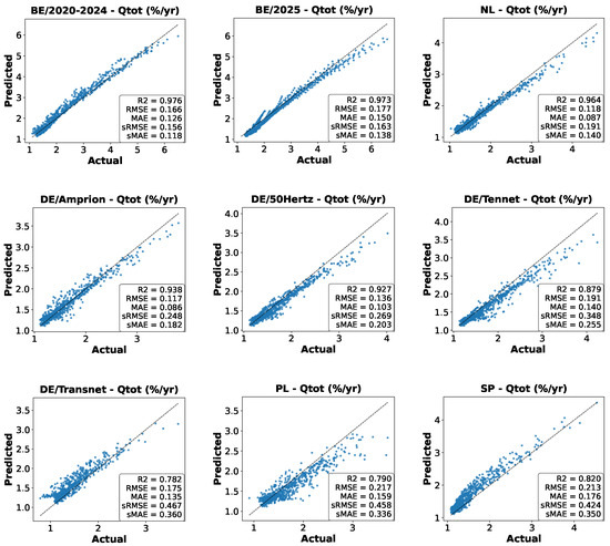
Figure 2. Predicted–actual parity plots for total capacity loss ($Q_{\mathrm{tot}}$) under the Ridge model across all entities. Tight alignment with the 1:1 line indicates strong fidelity and transfer. Belgium, the Netherlands, and Amprion exhibit the closest agreement; TenneT and 50 Hertz remain solid, while Spain and TransnetBW show modest upper-tail dispersion consistent with their higher RMSE. Insets report entity-level $R^2$/MAE/RMSE/sMAE/sRMSE.

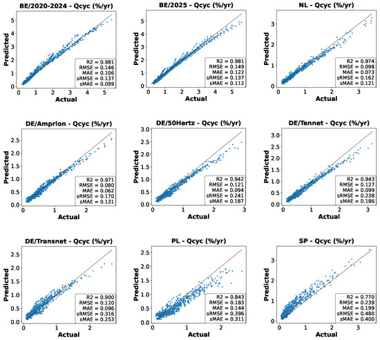
Figure 3. Predicted–actual parity plots for cyclic capacity loss ($Q_{\mathrm{cyc}}$) under the Ridge model across BE (Elia, Belgium), NL (TenneT NL, Netherlands), PL (PSE, Poland), SP (REE, Spain), and the four German TSOs (50 Hertz, Amprion, TenneT DE, TransnetBW). Tight clustering around the 1:1 line indicates strong fidelity. Agreement is closest for Belgium, the Netherlands, and Amprion; 50 Hertz and TenneT DE remain solid, while Spain and Poland (and, to a lesser extent, TransnetBW) exhibit upper-tail dispersion consistent with higher RMSE. Insets report entity-level $R^2$/MAE/RMSE/sMAE/sRMSE.

3.4. Cross-Behaviour Analysis of Degradation and Regime Balance

This section synthesises, for each TSO, the behaviour of the annual cycle and calendar capacity loss, $Q_{\mathrm{cyc}}$ and $Q_{\mathrm{cal}}$, as a function of the $E/P$. Figure 4 compares $Q_{\mathrm{cyc}}$, $Q_{\mathrm{cal}}$, and the total loss $Q_{\mathrm{tot}}$ for system-imbalance portfolio operation across all countries/TSOs as functions of $P_{max}$, DoD, and $E/P$. From the empirical $Q_{\mathrm{cyc}}$–$Q_{\mathrm{cal}}$–$E/P$ panels, three operating bands are delineated: cycle-dominant, mixed/balanced, and calendar-dominant, with the corresponding TSO-level regime boundaries summarised in Table 4. Here, “dominant” denotes a clear separation in magnitude, whereas the mixed band reflects comparable contributions. The reported ranges are approximate and are read from stable visual patterns along the surface perimeters; the accompanying notes summarise how higher DoD and $P_{max}$ shift these thresholds.

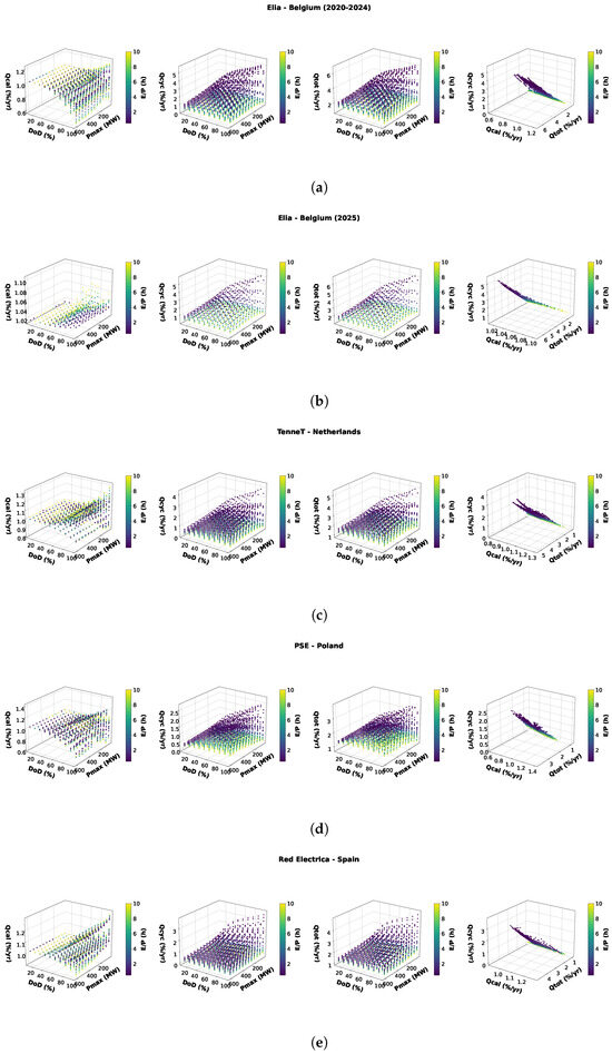
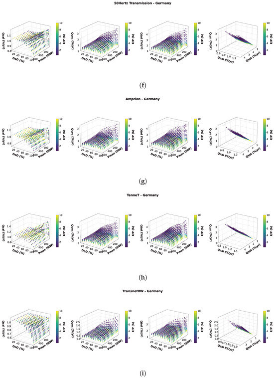
Figure 4. (a–e) Cross-behaviour of $Q_{\mathrm{cal}}$, $Q_{\mathrm{cyc}}$, and $Q_{\mathrm{tot}}$ versus $P_{max}$, depth of discharge (DoD), and $E/P$ (non-German entities). Panels: (a) Belgium—Elia (2020-2024); (b) Belgium—Elia (2025, hold-out); (c) Netherlands—TenneT NL; (d) Poland—PSE; (e) Spain—REE. Each panel shows $Q_{\mathrm{cal}}$, $Q_{\mathrm{cyc}}$, and $Q_{\mathrm{tot}}$ (left to right), with colour indicating $E/P$. (f–i) Cross-behaviour of $Q_{\mathrm{cal}}$, $Q_{\mathrm{cyc}}$, and $Q_{\mathrm{tot}}$ versus $P_{max}$, depth of discharge (DoD), and $E/P$ (German TSOs). Panels: (f) Germany—50 Hertz; (g) Germany—Amprion; (h) Germany—TenneT DE; (i) Germany—TransnetBW.

Table 4. Country/TSO-level balance between cyclic and calendar degradation.

TSO (Country)	${\mathit{Q}}_{\mathbf{cyc}}$-dom. $\mathit{E}/\mathit{P}$ Band	Mixed/ Balanced	${\mathit{Q}}_{\mathbf{cal}}$-dom. $\mathit{E}/\mathit{P}$ Band	Sensitivity (DoD/${\mathit{P}}_{max}$)
Elia (BE)	≤3 h	3–6 h	≥6 h	Higher DoD and $P_{max}$ extend $Q_{\mathrm{cyc}}$ dominance by ∼0.5–1 h.
TenneT NL (NL)	≤3 h	3–6 h	≥6 h	Similarly to BE; the mixed band widens at high DoD.
PSE (PL)	≤3.5–4 h	∼4–6.5 h	≥6.5 h	Most right-shifted thresholds; heavy cycling sustains $Q_{\mathrm{cyc}}$ at larger $E/P$.
REE (ES)	≤3 h	3–6 h	≥6 h	Mixed band broad at high DoD; otherwise near the canonical 3/6 h split.
50 Hertz (DE)	≤3 h	3–6 h	≥6 h	Canonical split; small right shift under high DoD/$P_{max}$.
Amprion (DE)	≤3.5–4 h	∼4–6.5 h	≥6.5 h	Similarly to PL: prolonged $Q_{\mathrm{cyc}}$ dominance to higher $E/P$.
TenneT DE (DE)	≤3 h	3–6 h	≥6 h	Near-canonical; thresholds are slightly elastic with DoD.
TransnetBW (DE)	≤3 h	3–6 h	≥6 h	Near-canonical; minimal shift.

At the European level (all TSOs aggregated), regime boundaries are remarkably consistent, with predictable elasticity under heavier cycling (higher DoD and $P_{max}$). Table 5 condenses the operating bands, typical behaviours, and design implications.

Table 5. EU-level operating bands (all TSOs aggregated).

$\mathit{E}/\mathit{P}$ Band (h)	Dominant	Typical Behaviour
≤3 h (up to ∼3.5–4 h under heavy cycling)	$Q_{\mathrm{cyc}}$	High throughput; $Q_{\mathrm{cyc}}$ is large (≈1.5–4) and $Q_{\mathrm{cal}}$ is low (≈0.9–1.1).
∼3–6 h	Mixed	$Q_{\mathrm{cyc}}$ decreases with $E/P$ while $Q_{\mathrm{cal}}$ increases modestly; magnitudes are comparable (balance region).
≥6 h (≳ 6–6.5 h under heavy cycling)	$Q_{\mathrm{cal}}$	Low cycling; $Q_{\mathrm{cal}}\approx 1.1$–1.3 dominates, while $Q_{\mathrm{cyc}}\approx 0$–1.

Across TSOs, $\mathrm{E}/\mathrm{P}\approx 3\mathrm{h}$ marks the onset of a mixed regime from a $Q_{\mathrm{cyc}}$-dominated one; $\mathrm{E}/\mathrm{P}\approx 6\mathrm{h}$ marks the transition to $Q_{\mathrm{cal}}$-dominated behaviour. Depth of discharge and $P_{max}$ reshape these boundaries: higher DoD and $P_{max}$ (a) raise $Q_{\mathrm{cyc}}$ monotonically, most strongly at low $E/P$ (high effective C-rate), and (b) shift the $E/P$ thresholds right by ∼0.5–1 h (most visible for PL and DE–Amprion), because heavier cycling keeps $Q_{\mathrm{cyc}}$ relevant at longer duration. In contrast, $Q_{\mathrm{cal}}$ is nearly insensitive to $P_{max}$, increases only mildly with DoD, and grows with $E/P$ owing to longer dwell at elevated SOC; thus at $\mathrm{E}/\mathrm{P}\gtrsim 6–8\mathrm{h}$ with DoD $\lesssim 40–50\%$ and moderate $P_{max}$, $Q_{\mathrm{cal}}$ typically exceeds $Q_{\mathrm{cyc}}$.

Quantitatively, three planning envelopes at $25 °\mathrm{C}$ summarise cross-entity behaviour:

(i)

Cycling-leaning $\left(\mathrm{E}/\mathrm{P}\le 3\mathrm{h};\mathrm{DoD}\ge 70\%;P_{max}\mathrm{high}\right)$: $Q_{\mathrm{cal}}\approx 1.0–1.3\%/\mathrm{yr}$, $Q_{\mathrm{cyc}}\approx 2.0–4.0\%/\mathrm{yr}$ (up to ∼$6.5\%/\mathrm{yr}$ in the most severe corner), $Q_{\mathrm{tot}}\approx 3.0–5.0+\%/\mathrm{yr}$.

(ii)

Balanced-regime $\left(\mathrm{E}/\mathrm{P}\approx 4–6\mathrm{h};\mathrm{DoD}\approx 50–70\%\right)$: $Q_{\mathrm{cal}}\approx 1.0–1.4\%/\mathrm{yr}$, $Q_{\mathrm{cyc}}\approx 0.8–1.8\%/\mathrm{yr}$, $Q_{\mathrm{tot}}\approx 1.8–3.2\%/\mathrm{yr}$.

(iii)

Calendar-leaning $\left(\mathrm{E}/\mathrm{P}\mathrm{high};\mathrm{DoD}\mathrm{moderate}/\mathrm{low};P_{max}\mathrm{moderate}\right)$: $Q_{\mathrm{cal}}\approx 1.0–1.5\%/\mathrm{yr}$, $Q_{\mathrm{cyc}}\approx 0.4–1.0\%/\mathrm{yr}$, $Q_{\mathrm{tot}}\approx 1.5–2.5\%/\mathrm{yr}$.

For imbalance management, sizing purely for high availability to cover volatile deviations pushes designs to larger $E/P$, improving coverage but moving assets into calendar-dominated ageing; sizing too small (low $E/P$) maximises cycling opportunity but risks coverage shortfalls and shifts wear towards $Q_{\mathrm{cyc}}$. A portfolio-level compromise of $\mathrm{E}/\mathrm{P}\sim 4–5.5\mathrm{h}$ sits squarely in the EU-wide balance region; operators can then steer the dominant wear mode via operational DoD while maintaining availability without a step change in lifetime drivers.

4. Conclusions and Context-Specific Recommendations

This work develops a compact, coefficientised degradation model for utility-scale LFP BESS operated under European system-imbalance conditions at 25 °C. The principal contribution is an auditable, scenario-parameterised representation of annual capacity loss that yields $Q_{\mathrm{cyc}}$, $Q_{\mathrm{cal}}$, and $Q_{\mathrm{tot}}$ as explicit functions of $E/P$, $P_{max}$, DoD, daily cycling intensity $N_{\mathrm{cyc}}$, and SOC bounds ($SO{C}_{min}$, $SO{C}_{max}$). By expressing degradation in coefficient form, the proposed model is directly usable as a transparent benchmark for system-imbalance techno-economic assessment and planning across EU jurisdictions where detailed electro-thermal telemetry is unavailable.

A second-degree polynomial specification with standardised inputs was evaluated across multiple linear estimators. Ridge regression ($\alpha ={10}^{-3}$) provided the most reliable generalisation across entities, consistent with a degradation signal distributed across correlated quadratic and interaction terms. Cross-entity testing (Table 2) confirms robust transferability across TSOs, and a full-year external hold-out (Belgium, 2025) provides an additional out-of-sample validation of the fitted response surfaces.

Beyond predictive performance, the fitted surfaces reveal consistent regime-level structure across countries and TSOs. Cycling-induced loss $Q_{\mathrm{cyc}}$ intensifies at low $E/P$ (high effective C-rate), higher $P_{max}$, and deeper DoD, whereas calendar-induced loss $Q_{\mathrm{cal}}$ increases with sustained SOC dwell and is therefore promoted by higher $E/P$ and elevated SOC operation. Consequently, $Q_{\mathrm{tot}}$ transitions from cycling-dominant behaviour at low $E/P$ to calendar-dominant behaviour at high $E/P$, with an intermediate mixed regime. At the EU level, this yields a practical sizing interpretation: $E/P\lesssim 3$ h is predominantly cycling-driven, $E/P\approx 3$–6 h is mixed, and $E/P\gtrsim 6$ h is predominantly calendar-driven, with the boundaries shifting with stress intensity (DoD and $P_{max}$).

Actionable Recommendations

(a)

Size within the mixed regime where possible: For stand-alone imbalance duty, $E/P\approx 4$–5.5 h provides a balanced operating region in which availability is improved without a step change toward calendar-dominant ageing. Selections of $E/P\ge 6$ h should be justified by explicit availability requirements, whereas $E/P\le 3$ h should be supported by portfolio-level coverage of large excursions.

(b)

Prioritise disciplined SOC policy: The SOC window is a dominant operational lever. Avoid high-SOC dwell and excessively wide windows; favour mid-SOC parking in the absence of events and maintain a conservative $SO{C}_{min}$ consistent with the required discharge headroom.

(c)

Manage cycling stress under sustained deviations: Limit prolonged deep cycling by constraining effective DoD and moderating $P_{max}$ during extended imbalance events. Where feasible, distribute correction through more frequent shallow actions rather than infrequent deep cycles to reduce $Q_{\mathrm{cyc}}$.

(d)

Use the coefficientised model as a TEA benchmark: Techno-economic studies for imbalance services should represent both cycle and calendar ageing. Where detailed duty-cycle or thermal data are not available, the coefficientised outputs provided here can be applied as a transparent benchmark for annual degradation, using $Q_{\mathrm{cyc}}$, $Q_{\mathrm{tot}}$, and $Q_{\mathrm{cal}}=Q_{\mathrm{tot}}-Q_{\mathrm{cyc}}$.

The framework is TEA-ready: the coefficientised equations support scenario screening, sizing studies, and SOC-policy design for BRP imbalance portfolios, and they can be embedded in optimisation workflows that balance availability, revenue, and lifetime cost. Feature-importance results (Appendix B) confirm SOC-window terms as dominant drivers, followed by $E/P$ and its SOC interactions, with throughput-related interactions becoming more relevant under high-stress operation.

Two scope limitations remain. First, temperature is fixed at 25 °C, reflecting the common assumption that utility-scale, containerised BESS employ thermal-management systems to maintain operation near a nominal setpoint; future work may extend the framework to explicitly quantify deviations from this assumption. Second, while cross-entity generalisation is strong for imbalance duty, validation for other duty types (e.g., peak shaving and reserves) is left for future work. A focused next step is to embed the degradation model in a techno-economic optimisation that jointly prices cycle and calendar ageing and quantifies the marginal cost of availability across historical imbalance traces.

Appendix A.1. Cyclic Loss Model ${\widehat{Q}}_{\mathrm{cyc}}$

Table A1. Ridge coefficients for the cyclic loss model ${\widehat{Q}}_{\mathrm{cyc}}$ (degree-2).

Symbol	Term	Value
$a_0$	Intercept	0.43370504
$a_1$	$E/P$	−0.037743268
$a_2$	$P_{max}$	3.9176498 × 10−5
$a_3$	$N_{\mathrm{cyc}}$	0.001487032
$a_4$	$\mathrm{DoD}$	0.0010598648
$a_5$	$SO{C}_{min}$	−0.21197298
$a_6$	$SO{C}_{max}$	0.21197298
$a_7$	${(E/P)}^2$	0.0068779559
$a_8$	$(E/P)P_{max}$	2.3831506 × 10−5
$a_9$	$(E/P)N_{\mathrm{cyc}}$	−0.00033347328
$a_{10}$	$(E/P)\mathrm{DoD}$	−0.00057625259
$a_{11}$	$(E/P)SO{C}_{min}$	−0.033087238
$a_{12}$	$(E/P)SO{C}_{max}$	−0.052017935
$a_{13}$	$P_{max}^2$	−5.4467615 × 10−7
$a_{14}$	$P_{max}{N}_{\mathrm{cyc}}$	−8.8147812 × 10−7
$a_{15}$	$P_{max}\mathrm{DoD}$	−8.4894949 × 10−8
$a_{16}$	$P_{max}SO{C}_{min}$	0.00015575948
$a_{17}$	$P_{max}SO{C}_{max}$	2.4021368 × 10−5
$a_{18}$	$N_{\mathrm{cyc}}^2$	−1.5267926 × 10−6
$a_{19}$	$N_{\mathrm{cyc}}\mathrm{DoD}$	2.0586156 × 10−5
$a_{20}$	$N_{\mathrm{cyc}}SO{C}_{min}$	0.00321675
$a_{21}$	$N_{\mathrm{cyc}}SO{C}_{max}$	0.0017971117
$a_{22}$	${\mathrm{DoD}}^2$	5.6723442 × 10−6
$a_{23}$	$\mathrm{DoD}SO{C}_{min}$	0.0094170521
$a_{24}$	$\mathrm{DoD}SO{C}_{max}$	0.00079726299
$a_{25}$	$SO{C}_{min}^2$	−0.63844033
$a_{26}$	$SO{C}_{min}SO{C}_{max}$	−0.22689383
$a_{27}$	$SO{C}_{max}^2$	0.11757815

Table A1. Ridge coefficients for the cyclic loss model ${\widehat{Q}}_{\mathrm{cyc}}$ (degree-2).

Symbol	Term	Value
$a_0$	Intercept	0.43370504
$a_1$	$E/P$	−0.037743268
$a_2$	$P_{max}$	3.9176498 × 10−5
$a_3$	$N_{\mathrm{cyc}}$	0.001487032
$a_4$	$\mathrm{DoD}$	0.0010598648
$a_5$	$SO{C}_{min}$	−0.21197298
$a_6$	$SO{C}_{max}$	0.21197298
$a_7$	${(E/P)}^2$	0.0068779559
$a_8$	$(E/P)P_{max}$	2.3831506 × 10−5
$a_9$	$(E/P)N_{\mathrm{cyc}}$	−0.00033347328
$a_{10}$	$(E/P)\mathrm{DoD}$	−0.00057625259
$a_{11}$	$(E/P)SO{C}_{min}$	−0.033087238
$a_{12}$	$(E/P)SO{C}_{max}$	−0.052017935
$a_{13}$	$P_{max}^2$	−5.4467615 × 10−7
$a_{14}$	$P_{max}{N}_{\mathrm{cyc}}$	−8.8147812 × 10−7
$a_{15}$	$P_{max}\mathrm{DoD}$	−8.4894949 × 10−8
$a_{16}$	$P_{max}SO{C}_{min}$	0.00015575948
$a_{17}$	$P_{max}SO{C}_{max}$	2.4021368 × 10−5
$a_{18}$	$N_{\mathrm{cyc}}^2$	−1.5267926 × 10−6
$a_{19}$	$N_{\mathrm{cyc}}\mathrm{DoD}$	2.0586156 × 10−5
$a_{20}$	$N_{\mathrm{cyc}}SO{C}_{min}$	0.00321675
$a_{21}$	$N_{\mathrm{cyc}}SO{C}_{max}$	0.0017971117
$a_{22}$	${\mathrm{DoD}}^2$	5.6723442 × 10−6
$a_{23}$	$\mathrm{DoD}SO{C}_{min}$	0.0094170521
$a_{24}$	$\mathrm{DoD}SO{C}_{max}$	0.00079726299
$a_{25}$	$SO{C}_{min}^2$	−0.63844033
$a_{26}$	$SO{C}_{min}SO{C}_{max}$	−0.22689383
$a_{27}$	$SO{C}_{max}^2$	0.11757815

Appendix A.2. Total Loss Model ${\widehat{Q}}_{\mathrm{tot}}$

Table A2. Ridge coefficients for the total loss model ${\widehat{Q}}_{\mathrm{tot}}$ (degree-2).

Symbol	Term	Value
$b_0$	Intercept	1.417728
$b_1$	$E/P$	−0.035978105
$b_2$	$P_{max}$	6.6073963 × 10−5
$b_3$	$N_{\mathrm{cyc}}$	0.0015216873
$b_4$	$\mathrm{DoD}$	0.0010786251
$b_5$	$SO{C}_{min}$	−0.21572504
$b_6$	$SO{C}_{max}$	0.21572501
$b_7$	${(E/P)}^2$	0.0067200451
$b_8$	$(E/P)P_{max}$	1.8052712 × 10−5
$b_9$	$(E/P)N_{\mathrm{cyc}}$	−0.00038919497
$b_{10}$	$(E/P)\mathrm{DoD}$	−0.00057379236
$b_{11}$	$(E/P)SO{C}_{min}$	−0.025563053
$b_{12}$	$(E/P)SO{C}_{max}$	−0.050574177
$b_{13}$	$P_{max}^2$	−5.9769256 × 10−7
$b_{14}$	$P_{max}{N}_{\mathrm{cyc}}$	−1.0815026 × 10−6
$b_{15}$	$P_{max}\mathrm{DoD}$	1.8252497 × 10−8
$b_{16}$	$P_{max}SO{C}_{min}$	0.00022469141
$b_{17}$	$P_{max}SO{C}_{max}$	4.8399153 × 10−5
$b_{18}$	$N_{\mathrm{cyc}}^2$	−1.58117 × 10−6
$b_{19}$	$N_{\mathrm{cyc}}\mathrm{DoD}$	2.0749117 × 10−5
$b_{20}$	$N_{\mathrm{cyc}}SO{C}_{min}$	0.0035044117
$b_{21}$	$N_{\mathrm{cyc}}SO{C}_{max}$	0.001826607
$b_{22}$	${\mathrm{DoD}}^2$	5.6479658 × 10−6
$b_{23}$	$\mathrm{DoD}SO{C}_{min}$	0.010020273
$b_{24}$	$\mathrm{DoD}SO{C}_{max}$	0.00080428759
$b_{25}$	$SO{C}_{min}^2$	−0.65694676
$b_{26}$	$SO{C}_{min}SO{C}_{max}$	−0.22591869
$b_{27}$	$SO{C}_{max}^2$	0.11900439

Table A2. Ridge coefficients for the total loss model ${\widehat{Q}}_{\mathrm{tot}}$ (degree-2).

Symbol	Term	Value
$b_0$	Intercept	1.417728
$b_1$	$E/P$	−0.035978105
$b_2$	$P_{max}$	6.6073963 × 10−5
$b_3$	$N_{\mathrm{cyc}}$	0.0015216873
$b_4$	$\mathrm{DoD}$	0.0010786251
$b_5$	$SO{C}_{min}$	−0.21572504
$b_6$	$SO{C}_{max}$	0.21572501
$b_7$	${(E/P)}^2$	0.0067200451
$b_8$	$(E/P)P_{max}$	1.8052712 × 10−5
$b_9$	$(E/P)N_{\mathrm{cyc}}$	−0.00038919497
$b_{10}$	$(E/P)\mathrm{DoD}$	−0.00057379236
$b_{11}$	$(E/P)SO{C}_{min}$	−0.025563053
$b_{12}$	$(E/P)SO{C}_{max}$	−0.050574177
$b_{13}$	$P_{max}^2$	−5.9769256 × 10−7
$b_{14}$	$P_{max}{N}_{\mathrm{cyc}}$	−1.0815026 × 10−6
$b_{15}$	$P_{max}\mathrm{DoD}$	1.8252497 × 10−8
$b_{16}$	$P_{max}SO{C}_{min}$	0.00022469141
$b_{17}$	$P_{max}SO{C}_{max}$	4.8399153 × 10−5
$b_{18}$	$N_{\mathrm{cyc}}^2$	−1.58117 × 10−6
$b_{19}$	$N_{\mathrm{cyc}}\mathrm{DoD}$	2.0749117 × 10−5
$b_{20}$	$N_{\mathrm{cyc}}SO{C}_{min}$	0.0035044117
$b_{21}$	$N_{\mathrm{cyc}}SO{C}_{max}$	0.001826607
$b_{22}$	${\mathrm{DoD}}^2$	5.6479658 × 10−6
$b_{23}$	$\mathrm{DoD}SO{C}_{min}$	0.010020273
$b_{24}$	$\mathrm{DoD}SO{C}_{max}$	0.00080428759
$b_{25}$	$SO{C}_{min}^2$	−0.65694676
$b_{26}$	$SO{C}_{min}SO{C}_{max}$	−0.22591869
$b_{27}$	$SO{C}_{max}^2$	0.11900439

References

- European Commission, Directorate-General for Energy. Key Facts on Energy Storage. European Commission—Energy. 2025. Available online: https://energy.ec.europa.eu/topics/research-and-technology/energy-storage/key-facts-energy-storage_en (accessed on 5 August 2025).
- European Parliament and the Council of the European Union. Regulation (EU) 2019/943 of 5 June 2019 on the internal market for electricity (recast). Off. J. Eur. Union 2019, 158, 54–124. [Google Scholar]
- European Commission. Commission Regulation (EU) 2017/2195 of 23 November 2017 establishing a guideline on electricity balancing (EBGL). Off. J. Eur. Union 2017, 312, 6–53. [Google Scholar]
- ENTSO-E; EFET; ebIX. The Harmonised Electricity Market Role Model; Version 2020-01; ENTSO-E: Brussels, Belgium, 2020. [Google Scholar]
- Chen, T.; Li, M.; Bae, J. Recent Advances in Lithium Iron Phosphate Battery Technology: A Comprehensive Review. Batteries 2024, 10, 424. [Google Scholar] [CrossRef]
- Yarimca, G.; Cetkin, E. Review of Cell Level Battery (Calendar and Cycling) Aging Models: Electric Vehicles. Batteries 2024, 10, 374. [Google Scholar] [CrossRef]
- Lam, V.N.; Cui, X.; Stroebl, F.; Uppaluri, M.; Onori, S.; Chueh, W.C. A decade of insights: Delving into calendar aging trends and implications. Joule 2025, 9, 101796. [Google Scholar] [CrossRef]
- García-Miguel, P.L.C.; Alonso-Martínez, J.; Arnaltes Gómez, S.; García Plaza, M.; Asensio, A.P. A review on the degradation implementation for the operation of battery energy storage systems. Batteries 2022, 8, 110. [Google Scholar] [CrossRef]
- Wankmüller, F.; Thimmapuram, P.R.; Gallagher, K.G.; Botterud, A. Impact of battery degradation on energy arbitrage revenue of grid-level energy storage. J. Energy Storage 2017, 10, 56–66. [Google Scholar] [CrossRef]
- Schade, C.; Egging-Bratseth, R. Battery degradation: Impact on economic dispatch. Energy Storage 2024, 6, e588. [Google Scholar] [CrossRef]
- Reniers, J.M.; Mulder, G.; Ober-Blöbaum, S.; Howey, D.A. Improving optimal control of grid-connected lithium-ion batteries through more accurate battery and degradation modelling. arXiv 2018, arXiv:1710.04552v3. [Google Scholar] [CrossRef]
- Sui, H.; Zhang, X.; Qin, Y.; Chen, L.; Liu, L. The degradation behavior of LiFePO4/C batteries during long-term calendar aging. Energies 2021, 14, 1732. [Google Scholar] [CrossRef]
- Birkl, C.R.; Howey, D.A. Model identification and parameter estimation for LiFePO4 batteries. In Proceedings of the IET Hybrid and Electric Vehicles Conference 2013, London, UK, 6–7 November 2013. [Google Scholar] [CrossRef]
- Alavi, B.N.; Birkl, C.R.; Howey, D.A. Time-domain fitting of battery electrochemical impedance models. J. Power Sources 2015, 288, 345–352. [Google Scholar] [CrossRef]
- O’Kane, S.E.J.; Ai, W.; Madabattula, G.; Alonso-Alvarez, D.; Timms, R.; Sulzer, V.; Edge, J.S.; Wu, B.; Offer, G.J.; Marinescu, M. Lithium-ion battery degradation: How to model it. Phys. Chem. Chem. Phys. 2022, 24, 7909–7922. [Google Scholar] [CrossRef] [PubMed]
- Collath, M.; Cornejo, A.; Engwerth, S.; Hesse, H.C.; Jossen, A. Increasing the lifetime profitability of battery energy storage systems through aging aware operation. Appl. Energy 2023, 348, 121531. [Google Scholar] [CrossRef]
- Elia Group. Imbalance Prices per Quarter-Hour (Historical Data—Up to 22/05/2024); Dataset ID: Ods047; Elia Open Data Portal: Brussels, Belgium, 2025. [Google Scholar]
- Elia Group. Imbalance Prices per Quarter-Hour (Historical Data as of 22/05/2024); Dataset ID: Ods134; Elia Open Data Portal: Brussels, Belgium, 2025. [Google Scholar]
- Elia Group. Imbalance Prices per Quarter-Hour (Near Real-Time); Dataset ID: Ods162; Elia Open Data Portal: Brussels, Belgium, 2025. [Google Scholar]
- TenneT TSO B.V. Settlement Prices—Imbalance Prices per Balancing Time Unit (API); TenneT Developer Portal: Arnhem, The Netherlands, 2025. [Google Scholar]
- ENTSO-E Transparency Platform. Balancing → Imbalance (Price and Components; Total Imbalance)—Interactive Data View; ENTSO-E AISBL: Brussels, Belgium, 2025. [Google Scholar]
- Schimpe, M.; Truong, C.N.; Naumann, M.; Jossen, A.; Hesse, H.C.; Reniers, J.M.; Howey, D.A. Marginal costs of battery system operation in energy arbitrage based on energy losses and cell degradation. In Proceedings of the 2018 IEEE PES Innovative Smart Grid Technologies Europe (ISGT-Europe), Sarajevo, Bosnia and Herzegovina, 21–25 October 2018; IEEE: Piscataway, NJ, USA, 2018; pp. 1–6. [Google Scholar]
- Naumann, M.; Schimpe, M.; Keil, P.; Hesse, H.C.; Jossen, A. Analysis and modeling of calendar aging of a commercial LiFePO4/graphite cell. J. Energy Storage 2018, 17, 153–169. [Google Scholar] [CrossRef]
- Naumann, M.; Spingler, F.B.; Jossen, A. Analysis and modeling of cycle aging of a commercial LiFePO4/graphite cell. J. Power Sources 2020, 451, 227666. [Google Scholar] [CrossRef]
Disclaimer/Publisher’s Note: The statements, opinions and data contained in all publications are solely those of the individual author(s) and contributor(s) and not of MDPI and/or the editor(s). MDPI and/or the editor(s) disclaim responsibility for any injury to people or property resulting from any ideas, methods, instructions or products referred to in the content. |
© 2026 by the authors. Licensee MDPI, Basel, Switzerland. This article is an open access article distributed under the terms and conditions of the Creative Commons Attribution (CC BY) license.