Abstract
Proton exchange membrane fuel cells (PEMFCs) are ideal for fuel cell vehicles due to their high specific power, rapid start-up, and low operating temperatures. However, their limited lifespan presents a challenge for large-scale deployment. Accurate assessment of remaining useful life (RUL) is essential for enhancing longevity. Automotive PEMFC systems are complex and nonlinear, making lifespan prediction difficult. Recent studies suggest deep learning approaches hold promise for this task. This study proposes a novel EMD-TCN-GN algorithm, which, for the first time, integrates empirical mode decomposition (EMD), temporal convolutional network (TCN), and group normalization (GN) by using EMD to adaptively decompose non-stationary signals (such as voltage fluctuations), the dilated convolution of TCN to capture long-term dependencies, and combining GN to group-calibrate intrinsic mode function (IMF) features to solve the problems of modal aliasing and training instability. Parametric analysis shows optimal accuracy with the grouping parameter set to 4. Experimental validation, with a voltage lifetime threshold at 96% (3.228 V), shows the predicted degradation closely aligns with actual results. The model predicts voltage threshold times at 809 h and 876 h, compared to actual values of 807 h and 872 h, with a temporal prediction error margin of 0.250–0.460%. These results demonstrate the model’s high prediction fidelity and support proactive health management of PEMFC systems.
1. Introduction
With the extensive production and consumption of fossil fuels, the global climate problem has become increasingly serious [1]. Clean energies such as wind energy, solar energy, wave energy, and other renewable energies are favored by scientists and are widely regarded as effective substitutes for fossil energy. However, the inherent intermittency and volatility of these energies limit their stability and large-scale promotion in energy supply. In this context, hydrogen, as an important clean energy, shows great potential in the energy transition and is considered as one of the important ways to achieve deep decarbonization. Using the abovementioned energies for electrolytic water to produce hydrogen is not only an important hydrogen production method, but it can also deal effectively with the intermittency and volatility problems of renewable energies, thereby further promoting the utilization and development of clean energies [2]. Therefore, hydrogen energy has an undeniable strategic significance in solving the global climate problem and promoting the development of sustainable energy. In the field of hydrogen fuel cells, proton exchange membrane fuel cells (PEMFCs) and solid oxide fuel cells (SOFCs) are very widely used. However, compared with solid oxide fuel cells, proton exchange membrane fuel cells have significant advantages, especially in terms of efficiency, durability, and stability [3]. In terms of efficiency, proton exchange membrane fuel cells operate at lower temperatures (60–80 °C) compared to solid oxide fuel cells (700–1000 °C). This reduces the energy consumption of thermal management and enables the system to start up quickly. In terms of durability and stability, proton exchange membrane fuel cells have the ability to resist carbon corrosion under dynamic operating conditions. In contrast, solid oxide fuel cells suffer from problems such as nickel agglomeration and anode degradation in high-temperature environments. Moreover, proton exchange membrane fuel cells show stronger tolerance to frequent load cycles, which is a key requirement for automotive applications. In terms of service life, the utilization of carbon fuels in proton exchange membrane fuel cells can achieve a voltage retention rate of over 90% within 5000 h, which is better than the benchmark performance of solid oxide fuel cells under comparable conditions. Therefore, due to the abovementioned favorable characteristics, proton exchange membrane fuel cells (PEMFCs) are widely used in various fields such as fuel cell vehicles, railway locomotives, and ships.
However, the lifespan of proton exchange membrane fuel cells (PEMFCs) poses a significant barrier to their widespread application. The key to extending their lifespan lies in the accurate assessment of their remaining useful life (RUL) [4,5]. Current research on lifespan prediction methods for PEMFCs can be primarily categorized into three approaches: physics-based methods, data-driven methods, and hybrid prediction methods [6].
The method of predicting the lifespan of proton exchange membrane fuel cells (PEMFCs) based on physical methods mainly relies on internal mechanism models, empirical models, semi-mechanistic models, or semi-empirical models [7]. The advantages of these methods include requiring less data, high accuracy, and strong universality. Bressel et al. [8] proposed a degradation-based extended Kalman filter observer to estimate the remaining useful life (RUL) by deriving the degradation state of the internal health core of the battery. However, this method is limited to using a single degradation model for life estimation, resulting in a lower robustness of the model. Based on the voltage polarization loss model established in the literature [9], Jouin et al. [10] developed an accurate semi-mechanistic model for the power degradation of proton exchange membrane fuel cells. By integrating experimental data with the mechanistic model, they quantified the dynamic evolution law of key performance indicators (such as voltage decay rate, ohmic impedance rise, etc.) during the aging process, but did not fully consider the concentration polarization loss caused by the anode concentration gradient and the hydrogen loss caused by the cross-leakage of the proton exchange membrane, and this simplification may affect the prediction accuracy of the model under dynamic variable load conditions. Zhang et al. [11] developed a typical semi-empirical and semi-mechanistic model to analyze the design parameters based on the equivalent electrochemical impedance spectroscopy (EIS) equivalent circuit model. Through experimental data and expert knowledge, they established a fuel cell power self-recovery model. This multi-model method ensures a lower computational workload and improved prediction accuracy. In general, the model-based methods fully consider the influence of internal aging factors and external state variables on the output performance of PEMFCs and have the advantages of low data dependence and strong universality. However, they need to establish an accurate mechanism model, which requires an in-depth exploration of the aging mechanism of fuel cells. This significantly increases the complexity of the modeling process.
Data-driven methods do not require the construction of internal degradation models. Instead, they use historical data to build suitable behavior models for fault diagnosis and lifespan prediction. The advantages of this approach include its ability to handle various nonlinear relationships, flexibility in model construction, and high prediction accuracy [12]. However, such methods still face the “black-box” problem regarding PEMFC aging mechanisms and state changes, meaning they cannot reveal the relationships between internal parameters or provide useful insights for subsequent development and maintenance. Common types of data-driven methods in current research include statistical modeling, machine learning, deep learning, and hybrid learning [13]. Data-driven methods are based on statistical learning or machine learning (ML) algorithms to extract degradation pattern representations from massive fuel cell aging data, and then construct data-driven prediction models to achieve quantitative prediction of aging trends [14,15]. Literature [16] introduces a series of machine learning methods, including the linear regression model (LR), support vector regression model (SVR), decision tree regression (DT), and a multi-layer perceptron model (MLP). It also conducts a comparative analysis of their advantages and disadvantages in predicting capacitance, offering a new approach for the application of machine learning in materials. Deep learning, as an important branch of ML, has a strong learning ability and adaptability, and it has broad application prospects in the field of fuel cell degradation prediction [17]. Morando et al. [18] use the echo state network (ESN), combined with the prior knowledge of fault tolerance (FT) technology to estimate the remaining useful life (RUL). Li et al. [19] designed an RUL prediction method based on GRU, which generally performs better than conventional methods. He et al. [20] extract health indicators from the degradation voltage and use the long short-term memory network (LSTM) to predict future health indicators. Yi et al. [21] proposed an improved model of matrix long short-term memory (M-LSTM), which can enhance the global modeling ability of LSTM in complex nonlinear feature learning and long sequence data processing. Zhou et al. [22] applied convolutional neural network–bidirectional gated recurrent unit with attention mechanism (CNN-BiGRU-AM) for fuel cell fault prediction. The proposed method has a good performance in the remaining useful life prediction. Compared with the traditional machine learning prediction model, the short-term prediction performance of this fusion model has been significantly improved. Although the existing methods have good prediction accuracy, the accuracy of their prediction results depends on a large amount of high-quality data and effective prediction methods.
Since both physics-based and data-driven methods have their advantages and limitations, hybrid model prediction approaches combine the interpretability of internal parameters in physics-based models with the flexibility of data-driven methods to address unclear physical mechanisms. This hybridization allows for the treatment of ambiguous aspects of the system, making subsequent predictions more feasible. By integrating the strengths of both approaches, hybrid models improve the overall prediction accuracy. In existing research, three primary hybridization strategies have been identified: model-data hybrid-driven, data-data hybrid-driven, and multi-data-multi-model hybrid-driven modes. Mao et al. [23] developed a sensitivity and noise-resistant model to select the optimal sensor measurement combinations. These combinations were then used as inputs for an adaptive neuro-fuzzy inference system (ANFIS) to estimate voltage degradation in PEMFCs, thus investigating their performance decline. The data-data hybrid mode involves fitting the data and using this dimension of information in another data model for prediction, thereby improving prediction accuracy and robustness. Zhu et al. [24] proposed a B-GRU hybrid model by combining Bayesian theory and self-attention mechanisms. They first employed a random forest model to extract key feature parameters and then introduced these features into the B-GRU model, yielding favorable accuracy. Li et al. [25] extracted aging features from the polarization curve of the battery using a degradation empirical model, while simultaneously identifying aging features from the electrochemical impedance spectroscopy (EIS) data through a backpropagation neural network. By performing similarity analysis on these aging features, they improved results and reduced random errors. The final fusion of aging features was then incorporated into the model to accurately predict the aging state of PEMFCs. From a review of existing studies, it is clear that hybrid-driven approaches offer superior prediction accuracy compared to solely model-based or data-driven methods. However, this comes with the trade-offs of more complex models and longer computational times.
To address the challenges of high noise and instability in fuel cell data caused by complex operating conditions and electromagnetic interference, this study proposes an EMD-TCN hybrid framework that integrates empirical mode decomposition (EMD) and temporal convolutional network (TCN). This framework achieves high-precision lifetime prediction through three key innovations: (1) EMD separates high-frequency noise (e.g., transient load fluctuations) from low-frequency degradation trends (e.g., catalyst aging) to achieve adaptive multi-scale signal modeling; (2) group normalization (GN) calibrates multi-channel intrinsic mode function (IMF) features, suppresses mode mixing, and enhances the interpretability of degradation mechanisms (voltage attenuation, flow channel blockage); (3) the optimized group convolution in TCN improves computational efficiency while maintaining long-term dependency modeling based on dilated convolution. Mainstream models such as RNN, LSTM, and TCN are selected as the benchmark models for prediction. These models can effectively model the time dependence of the battery degradation process (such as the long-term trend of voltage attenuation and the short-term fluctuations of start–stop events) and the vanishing gradient problem, thereby maintaining their robustness in long time-series. They are classic models widely used in the current field. Taking these models as a benchmark provides a technical reference for the performance comparison of the new method (such as EMD-TCN) proposed in this paper. At the same time, its computational efficiency (single-step complexity) and the support of a mature toolchain ensure the engineering feasibility.
The structure of the remaining sections of this paper is as follows: Section 2 discusses the characteristics of steady-state and dynamic cycling conditions and performs filtering and smoothing of several strongly correlated feature parameters for denoising and reconstruction. Section 3 presents prediction models based on RNN, LSTM, TCN, and the EMD-based TCN model. In Section 4, a comparative analysis and summary of the predictions from different models are provided. Section 5 concludes the paper and offers perspectives for future research.
2. Data Source and Preprocessing
2.1. Data Source
In the research process, due to the consistency of the durability tests, the sealing of the fuel cell stack, and the relatively slow aging process of internal components such as the proton exchange membrane and the bipolar plates, it is difficult to select reasonable performance indicators for monitoring from within the stack. Therefore, external indicators are chosen to characterize the state [26]. To accurately predict the aging trend and lifespan status of proton exchange membrane fuel cells (PEMFCs), the team utilized the publicly available durability test dataset from the 2014 IEEE PHM Data [27] for model training and testing, the test bench is shown in Figure 1.
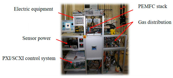
Figure 1.
2014 IEEE PHM Data Challenge Durability Test Bench [26].
Two sets of comparative durability experiments were designed in the text: ① group FC1 corresponds to the steady-state operation mode, with constant operating condition parameters (current density of 0.7 A/cm2, load current of 70 A) set. The experiment maintains constant conditions throughout the entire process, with a monitoring duration of 1154 h. ② Group FC2 applies dynamic disturbance conditions; in addition to the basic current density of (0.7 ± 0.07) A/cm2, a 5 kHz high-frequency triangular wave pulsating current is superimposed to simulate a complex electromagnetic environment. Based on the research goal of predicting the steady-state life of the fuel cell, the experimental data of Group FC1 is preferentially selected as the analysis basis. Table 1 details the stack structure parameters, and the monitoring indicator system covers gas path parameters (hydrogen/air flow and pressure), thermal management parameters (coolant temperature), and electrical parameters (output voltage, current, and voltage of each cell). By periodically collecting the polarization curve data of the two sets of stacks (Figure 2), it is found that under the same current condition, the voltage of the PEMFC decreases with the increase of the test time, indicating the aging of the proton exchange membrane fuel cell (PEMFCs). Based on the above phenomenon, the study selects the output voltage of the stack as the key parameter to characterize the health status of the PEMFC, which is used to construct the remaining useful life (RUL) prediction model.

Table 1.
FCL experimental fuel cell stack parameters.
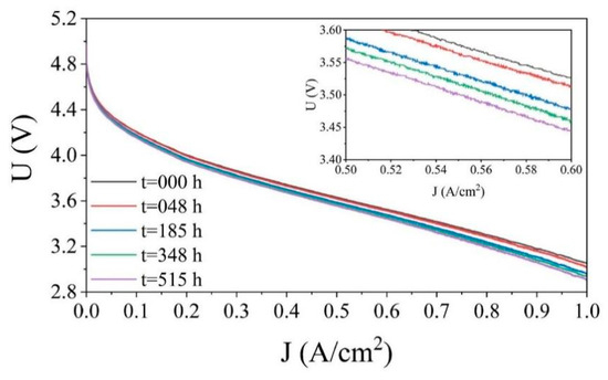
Figure 2.
Polarization curves of FC1.
2.2. Data Preprocessing
2.2.1. Data Processing Methods
Empirical Mode Decomposition (EMD)
Empirical mode decomposition (EMD) is a statistical analysis method that decomposes complex, variable, and irregular digital signals into several independent intrinsic mode functions (IMFs) and extracts data features from them, without the need to predefine basis functions or filters. EMD has wide applications in signal processing, time-series analysis, image processing, and other fields [27].
The IMF components reflect the variations in the local frequency and amplitude of the signal. Each decomposed IMF component must satisfy two characteristics. First, in the global data, the number of local maxima and local minima must be equal or differ by at most one, meaning the difference between the number of zero-crossings and extrema points is no greater than one [28]. Second, at any given time point, the average value of the signal—the average of the upper and lower envelopes, formed by the maxima and minima points—is zero. IMFs are adaptive and can automatically adjust to and extract important information based on the characteristics of the signal, making them well-suited for the analysis of nonlinear and nonstationary signals.
For the original time-series data, the EMD decomposition steps are:
First: extract extremum points and fit envelope curves. Extract all extremum points of x(t) and use interpolation methods (such as spline interpolation) to connect the local maxima and local minima, thereby obtaining the upper and lower envelope curves of the signal. These envelope curves represent the overall trend of the signal.
Second: calculate the local mean and intermediate signal. The local mean m(t) is the average of the upper and lower envelope curves. It is used to remove the overall trend of the signal, revealing the signal’s details. The intermediate signal r(t) is the difference between the original data and the local mean, which can be expressed as follows:
Third: determine whether the intermediate signal r(t) satisfies the aforementioned characteristics of an intrinsic mode function (IMF) component. If it does, record its values; if not, repeat the first and second steps until the component characteristics are met.
Reconstruct the signal: first, calculate the residual component u1(t), which is the difference between the original data and the first high-frequency component extracted during decomposition. This can be expressed as follows:
The signal u1(t), obtained from the initial decomposition, represents a low-frequency component relative to r1(t). Treating u1(t) as a new input signal, the decomposition process continues to generate subsequent components u2(t) and r2(t), until the residual component becomes either monotonic or constant. The EMD decomposition process terminates at this point. By summing all the intrinsic mode functions (IMFs) and adding back the removed local mean, the original signal can be reconstructed. This can be mathematically expressed as follows:
In the equation, uk(t) can be considered as the mean of the signal x(t), while rk(t) represents the IMF component, which refers to the high-frequency to low-frequency components of the original time-series data.
The performance degradation signals of fuel cells (such as voltage, current, temperature, etc.) have significant non-stationarity and nonlinearity. Traditional frequency-domain methods (such as Fourier transform and Wavelet transform) rely on preset basis functions or stationarity assumptions, making it difficult to effectively separate noise, working condition disturbances, and the real degradation trend. Empirical mode decomposition (EMD) decomposes the original signal into multiple intrinsic mode functions (IMFs) through an adaptive decomposition mechanism without the need for a priori basis function selection, which naturally fits the characteristics of the dynamic degradation data of fuel cells and greatly improves the prediction accuracy.
Discrete Wavelet Transform (DWT)
In the proton exchange membrane fuel cell (PEMFC) system, experimental data often exhibit non-stationary characteristics due to high-frequency oscillations. In this study, one-dimensional discrete wavelet transform (DWT) is used for signal denoising: the original signal is regarded as the highest scale, and through multi-scale decomposition, the scale function is used to approximate the low-frequency trend, while the wavelet function is introduced to characterize the high-frequency detail differences to achieve signal reconstruction. Compared with the Fourier transform, DWT suppresses noise interference based on the time-frequency localized window. Its core advantage lies in the adaptive separation of high-frequency oscillations (sub-scale resolution analysis) and low-frequency slowly varying features (frequency-domain compression representation) through scale scaling and translation operations, thereby accurately extracting the local dynamic characteristics of the data [29].
The wavelet is defined as a family of functions obtained by translating and scaling the mother wavelet and .
Thus, the wavelet is expressed as follows:
In the equation, a is the scaling factor, and b is the translation factor. Together, they allow the wavelet function to move along the time axis. The wavelet basis has finite energy and exhibits oscillatory characteristics, which enable it to maintain a specific shape within a finite time and decay rapidly outside that time interval. The wavelet transform is a method of transforming an analog signal into a representation accumulated using wavelet basis functions. The mathematical formula for the wavelet transform is given by the following equation:
In the equation, and are complex conjugates of each other.
The one-dimensional discrete wavelet transform (DWT) is used to discretize the continuous wavelet transform by introducing discrete translation and scaling parameters. It can be represented as follows:
In the equation, both a and b are multiples of 2j, .
The data processing methods are shown in Table 2.
Table 2.
Comparison of data processing methods.
2.2.2. The Specific Data Processing Process
The dataset collected by FC1 group consists of 3 files. After combining them, there are approximately 140,000 time-series data points. The voltage data are shown in Figure 3a. Due to the complexity and large volume of the data, directly inputting it into the model would significantly increase the computational load, reduce computational efficiency, and lead to potential overfitting during the computation process. Therefore, it is necessary to process the dataset [30]. First, interval sampling is performed, with the output voltage sampled every 70 s, resulting in 2000 sample sequences, as shown in Figure 3b. However, interval sampling causes the data to exhibit abrupt changes. To reduce the impact of noise and improve prediction accuracy, discrete wavelet transform (DWT) is used to smooth the interval-sampled data. The processed output voltage data are shown in Figure 3c. From the figure, it can be observed that after the denoising process, the voltage information retains the original voltage curve’s trend, the abnormal data are reduced, and the overall data are smoother, making it easier for subsequent model predictions.
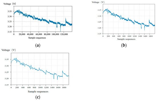
Figure 3.
FC1 voltage dataset preprocessing results: (a) original FC1 voltage data; (b) interval-sampled voltage data; (c) denoised and smoothed voltage data.
The preprocessed 2000 voltage time-series data points are divided into sliding windows. The sequence length (sequence_length) is set to 200, meaning that consecutive 200 data points are used as a training sample. The first 100 data points of each sample serve as the input data for the prediction model, while the last 100 data points are the true labels with predicted values. In total, 1900 training datasets and 1900 prediction datasets are accumulated. To explore the applicability of various prediction algorithms for PEMFC lifetime prediction, the dataset is divided into training and testing sets with ratios of 4:6, 6:4, and 8:2.
3. Lifetime Prediction Model Design
3.1. Voltage Prediction Algorithm Process
The voltage prediction experiment is shown in Figure 4 and consists of three parts: data preprocessing, model training, and model testing. The dataset used is the IEEE PHM Data Challenge durability testing public dataset mentioned earlier.
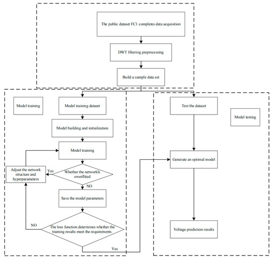
Figure 4.
PEMFC system voltage prediction process.
In the data preprocessing phase, the raw voltage data are first processed using DWT or EMD. Then, the data are divided into different proportions based on a preset ratio. In the model training phase, various deep learning models are constructed and initialized. The training set is fed into these models for training, and after each training session, the results are quantitatively evaluated. The model structure and hyperparameters are adjusted and optimized to obtain the best prediction model. In the model testing phase, the test set is fed into the optimal prediction model to compute the voltage prediction results. The efficiency and accuracy of the models are compared under different prediction methods.
Under the steady-state conditions in this study, the research team established a comprehensive evaluation index system. It mainly uses parameters such as the root mean square error (RMSE), the coefficient of determination (R2), and the difference between the predicted time and the actual time when the voltage reaches the decline threshold to construct a combined analysis index. In this way, it can evaluate the fitting degree of the model’s voltage trajectory (RMSE) and measure the model’s ability to explain voltage changes (R2) overall and capture the error at the critical node of the late stage of voltage attenuation locally. The calculation formulas for RMSE and R2 are as follows:
In the equation, the following is true:
: The i-th predicted value.
: The i-th true value.
n: The number of samples.
In the equation, the following is true:
: The i-th predicted value.
: The i-th true value.
: The mean of the true values.
n: The number of samples.
3.2. Environment Configuration
This training experiment uses the Python programming language, with the software environment set to VS Code and the optimizer set to Adam. The experimental environment configuration is shown in Table 3. To facilitate the comparison of prediction results across models, the number of iterations, hidden layer size, and sequence length are kept consistent. At the same time, to ensure the reliability of the prediction results and minimize random errors, each model undergoes three prediction runs. The RMSE, R2, and other evaluation metrics are calculated by averaging the results from the three predictions.
Table 3.
Experimental environment configuration.
3.3. Lifetime Prediction Model Based on Recurrent Neural Networks (RNNs)
Recurrent neural networks (RNNs) are capable of capturing sequential information and transmitting it through one or more cycles. The basic structure of an RNN includes one or more recurrent units, which repeat over time steps. At each time step, the RNN receives an input vector and a hidden state and outputs an output vector and an updated hidden state. The hidden state is updated at each time step based on the current input and the hidden state from the previous time step. Through cyclic connections, the RNN can propagate prior information to subsequent time steps, allowing it to retain and transfer important contextual information in the sequence. The basic structure of the RNN is shown in Figure 5.
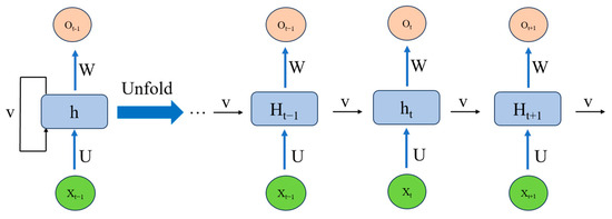
Figure 5.
RNN network structure.
In the model development stage, to suppress the overfitting tendency in the model prediction process, the dropout regularization technique [31] is introduced. This technique implements dynamic network structure optimization by randomly masking a specific proportion (such as 40%) of neuron nodes and their associated weights during the training stage. Through the dynamic random inactivation strategy in each training cycle, it realizes the implicit integration of multiple groups of sparse sub-networks, thereby avoiding repeated optimization of the fixed network architecture and effectively improving the generalization performance of the model for new samples. Its working mechanism is shown in Figure 6.
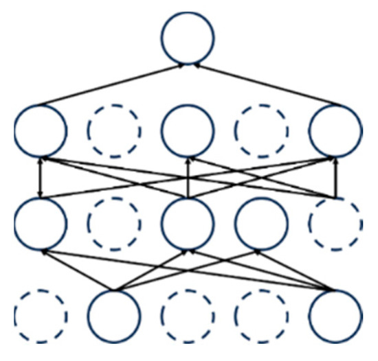
Figure 6.
Dropout technique diagram.
To ensure that the learning rate η can adaptively adjust while maintaining the adaptability and stability of each parameter, the Adam optimizer was chosen. The other configurations are as follows: the number of neurons in the hidden layers is 150, the dropout probability is 0.4, the activation function is ReLU, the number of iterations is 2000, and to balance training speed and generalization ability, the batch size is set to 64 for each iteration. The number of iterations is experimentally determined using the early stopping method, that is, the training stops when the performance of the model on the validation set no longer improves, and the final number is selected as 2000 iterations; parameters such as batch size are set according to the computer configuration. The prediction results are shown in Figure 7, and the model evaluation metrics are presented in Table 4.
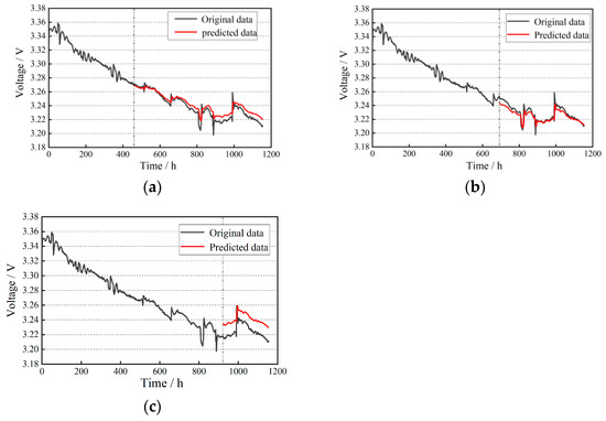
Figure 7.
RNN life prediction results: (a) training set ratio of 40%; (b) training set ratio of 60%; (c) training set ratio of 80%.
Table 4.
RNN life prediction evaluation metrics.
The analysis shows that with 80% of the data used for training, the RMSE of the RNN model decreased by 52.7% compared to 40%, and by 14.4% compared to 60%, while the R2 values increased by 64.3% and 45.5%, respectively. This indicates that a larger training dataset leads to better extraction of machine learning information, resulting in more accurate trend predictions. As seen in Figure 7b,c the training results exhibit slight gradient explosion, with the predictions gradually deviating from the normal values over time. This suggests inherent limitations of traditional RNN models, which are not easily parallelizable and are prone to gradient vanishing or explosion.
3.4. LSTM-Based Life Prediction Model
LSTM (long short-term memory) is an enhanced type of recurrent neural network (RNN) that incorporates a gating mechanism to handle complex data with strong temporal dependencies. This innovation addresses the weakness of traditional RNNs in dealing with long-term sequential dependencies. Through its gating mechanism, LSTM can effectively control the flow of information, enabling it to better capture and transmit long-term dependencies [32,33]. This makes LSTM highly effective in tasks such as language modeling, machine translation, and text generation in sequence data. The gating mechanism of LSTM includes the forget gate, input gate, and output gate, which autonomously learn and adjust the weights of input data to better control the flow of information and preserve important contextual information. The structure of its unit is shown in Figure 8 [34].
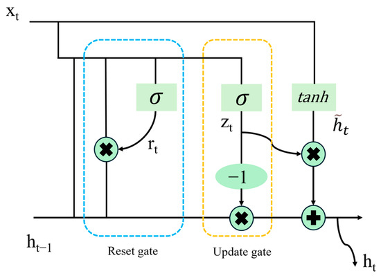
Figure 8.
LSTM unit structure.
On the basis of the LSTM algorithm architecture, to prevent overfitting in predictions, the dropout technique is also introduced. According to the conclusions of Bin et al. [35], a learning rate η = 0.01 and a dropout random deletion probability of 0.4 were selected to train the network. The number of neurons in the LSTM hidden layer is 150, the number of iterations is 2000, the learning rate decays every 50 epochs, and the learning rate decay rate is 0.2. The final prediction results are shown in Figure 9, and the model evaluation metrics are presented in Table 5.
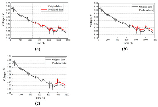
Figure 9.
LSTM life prediction results: (a) training set ratio of 40%; (b) training set ratio of 60%; (c) training set ratio of 80%.
Table 5.
LSTM life prediction evaluation metrics.
Analysis indicates that when the training set accounts for 80% of the data, the RMSE of the LSTM model decreases by 16.4% compared to 40%, while it slightly increases by 1.9% compared to 60%. The R2 value shows no significant difference, suggesting that the fitting capability of the LSTM model is less affected by the proportion of the training set. In the prediction phase, the voltage error gradually increases over time, which can be attributed to the lack of model-based correction of the prediction results, leading to the accumulation of errors.
3.5. Life Prediction Model Based on Temporal Convolutional Network (TCN)
Temporal convolutional network (TCN) is a neural network technique capable of effectively processing time-series data and transforming it into a predictive model. The TCN model is composed of multiple stacked 1D convolutional layers. The 1D convolution operation efficiently captures both global and local information from time-series data, offering higher parallelism and computational efficiency [36,37]. The structural unit of the TCN is shown in Figure 10.
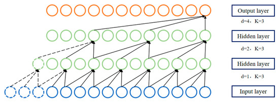
Figure 10.
TCN dilated convolutional structural unit.
The input and output of the convolutional layer are one-dimensional feature vector sequences of time-series data, where the features at each time step are obtained by performing convolution operations on local regions of the input sequence. An activation function is then applied to introduce nonlinearity. Typically, a global average pooling layer or a global max pooling layer is added at the end to extract the overall features of the time-series data. Subsequently, the extracted features are mapped to the final output through a fully connected layer.
Considering the length of the training dataset, the number of neurons in the TCN encoder input layer is set to 32, the number of neurons in the hidden layer is set to 64, and the size of the 1D convolutional kernel is set to 3. The number of neurons in the feedforward neural network is set to 128. The final prediction results are shown in Figure 11, and the model evaluation metrics are presented in Table 6.
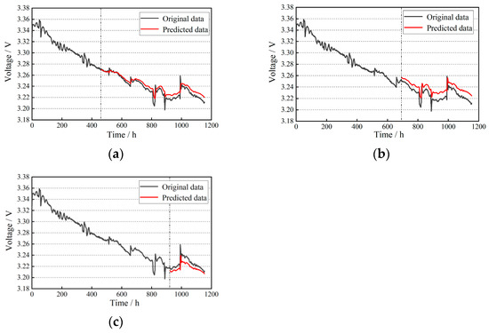
Figure 11.
TCN life prediction results: (a) training set ratio of 40%; (b) training set ratio of 60%; (c) training set ratio of 80%.
Table 6.
TCN life prediction evaluation metrics.
Analysis shows that when the training set accounts for 80% of the data, the RMSE of the TCN model decreased by 60.8% compared to 40%, and by 35.1% compared to 60%. The R2 values increased by 97.3% and 71.3%, respectively. In applications such as predicting fuel cell lifespan and other long-term time-series forecasting, the TCN model processes training data faster, offers more adjustable hyperparameters, and exhibits stronger adaptability and generalization ability.
3.6. Lifespan Prediction Model Based on EMD-TCN
To further improve the prediction accuracy of long-term time-series data for the PEMFC system, a novel data processing scheme based on empirical mode decomposition (EMD) is proposed. This approach demonstrates stronger adaptability when processing nonlinear and non-stationary signals. Therefore, an EMD-TCN fuel cell lifespan prediction model is introduced, with improvements made to the normalization layer of the TCN.
In the basic structure of the TCN model, the unit residual block consists of two identical internal convolutional units and a residual connection. The logical sequence processed by a single convolutional unit is as follows: causal convolution layer, normalization layer, activation function, and dropout layer. There are several types of normalization methods, including weight normalization (WN), group normalization (GN), batch normalization (BN), and instance normalization (IN) [38,39]. Compared to BN and IN, GN has lower computational complexity, and it more accurately shares statistical information within groups with fewer channels, thereby reducing the risk of overfitting and enhancing the model’s generalization ability. Therefore, in this experiment, the group normalization (GN) method is employed to improve the TCN, with the commonly used activation function of exponential linear unit (ReLU). The prediction process of the PEMFC lifespan based on the EMD-TCN (GN) model is shown in Figure 12.
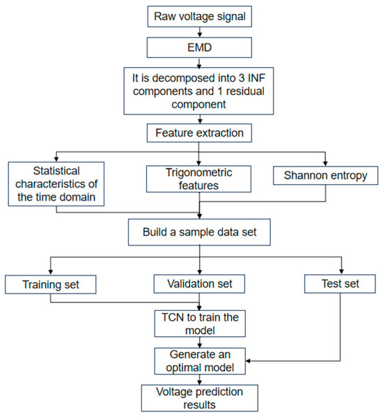
Figure 12.
PEMFC Prediction Process Based on EMD-TCN Model.
The specific steps for the prediction are as follows:
Classical modal decomposition: The original voltage data are decomposed into three intrinsic mode function (IMF) components and one residual component using empirical mode decomposition (EMD) with three layers. According to the previous experiments, to determine the number of decomposition layers, too few layers will lead to lower prediction accuracy, and too many layers will increase the computational complexity and also introduce unnecessary noise or false components.
Feature extraction: Seven statistical features are calculated for each of the four components, resulting in a 28-dimensional feature dataset.
TCN model: The features from the training set are normalized using min-max normalization. The normalized results are then used as inputs to the model, with the remaining lifetime percentage PPP (percentage of remaining performance) as the training label. The Adam optimizer is employed for model training. A random 20% of the data are used as a validation set to enhance the model’s generalization capability.
Test set validation: The trained optimal model is used to predict the remaining lifetime percentage based on the test set.
Following these steps, the preprocessed 2000 voltage time-series data are divided into a training set and a test set with a 6:4 ratio. The training set is used as input for the EMD decomposition, ultimately producing three IMF components and 1 residual component (res.).
The TCN (GN) model has a neuron count of 64, 32, 16, 8, and 1 in the residual connections from the first to the last layer. The design decreases the number of neurons (64 → 32 → 16 → 8 → 1). The first layer with 64 neurons captures the high-frequency details of the original voltage signal (such as millisecond-level load fluctuations), retains rich information through a wide number of channels, and achieves spatial dimension compression (reducing the risk of overfitting) and key feature enhancement (highlighting low-frequency patterns such as attenuation trends) by halving the number of neurons layer by layer. Finally, the output of one neuron (voltage prediction) meets the task requirements. With dilation rates of 1, 2, 4, 8, and 16, respectively. The expansion rate shows exponential growth (1 → 2 → 4 → 8 → 16). The underlying expansion rate of 1 (equivalent to conventional convolution) captures the influence of local fluctuations (such as start-stop impacts). The exponential expansion layer by layer makes the receptive field grow geometrically, matching the overall attenuation period. The convolution kernel size is 3, the activation function used is ReLU, and the batch size is 32. Compared with a small batch, the training stability is higher, and the convergence rate increases significantly; compared with a batch size of 64, its overfitting risk is smaller. A step size that is too short will result in the TCN model failing to learn sufficient data information, while a step size that is too long will increase the computational load, thereby reducing efficiency. Based on literature [40,41], the step size is set to 16. To evaluate the applicability of the TCN (GN) model in predicting the lifespan of PEMFC, TCN (WN) and TCN (BN) are used as control groups for experimental comparison. The prediction results are shown in Figure 13.
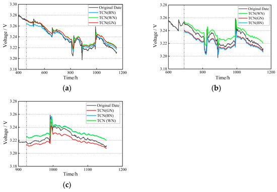
Figure 13.
TCN (WN), TCN (BN), TCN (GN) life prediction results: (a) training set ratio of 40%; (b) training set ratio of 60%; (c) training set ratio of 80%.
As can be seen from the figure, under different training conditions, the TCN (GN) model slightly outperforms TCN (WN) and TCN (BN) in terms of overall prediction accuracy across the entire prediction interval, yielding a more ideal fitting effect. Through quantitative analysis of model evaluation metrics, as shown in Table 7, the RMSE of TCN (GN) is consistently smaller than that of the other two models, and its R2 value is superior to that of the other two, further demonstrating that TCN (GN) can accurately share statistical information with fewer intra-group channels, has a lower risk of overfitting, and possesses stronger model generalization capabilities. This suggests that TCN (GN) is more capable of meeting the accuracy requirements for lifespan prediction.
Table 7.
TCN (WN), TCN (BN), TCN (GN) life prediction evaluation metrics.
In further research, the internal structural parameters of the TCN model were deeply explored, particularly focusing on the selection of normalization layers. However, based on the normalization features in the TCN group, suitable grouped convolutions can increase the network’s nonlinearity expression ability, help reduce the number of parameters, and improve computational accuracy. Depending on the dataset length, the grouping parameters were initially selected as 2, 4, and 8, referred to as TCN (GN-2), TCN (GN-4), and TCN (GN-8), respectively. Through experiments and cross-validation, the optimal grouping parameter combination was determined.
The data after modal decomposition were imported into each TCN model, and RMSE and R2 were calculated, with the prediction results shown in Table 8 and Figure 14. For the output voltage prediction results based on the EMD-improved TCN (GN-X) model, EMD-TCN (GN-4) outperforms TCN (GN-2) and TCN (GN-8) in 40%, 60%, and 80% training data proportions. When compared to the prediction results in literature [35], which used a similar method, that study demonstrated the best prediction performance when the grouping parameter was 2 (i.e., using the TCN (GN-2) model). This conclusion is inconsistent with the findings in this paper. Upon analysis, it is found that the voltage data used in this paper are an order of magnitude smaller than the bearing lifespan data in that study. With smaller datasets, smaller grouping parameters lead to higher variance. As the calculation of mean and variance is smaller, the normalization effect is not as effective as that of larger grouping parameters. Therefore, when using the TCN-based normalization model, it is important to select appropriate grouping parameters according to the specific application scenario and dataset characteristics in order to achieve the best normalization effect and computational efficiency.
Table 8.
The evaluation metrics of TCN with different GN.
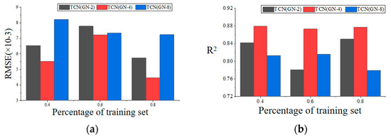
Figure 14.
Visualization comparison of prediction results across multiple models: (a) comparison of RMSE results; (b) comparison of R2 results.
4. Results and Discussion
To evaluate the performance of the proposed EMD-TCN voltage prediction model, a comparative analysis is conducted across various models, including traditional RNN, LSTM, as well as TCN (WN), TCN (BN), and TCN (GN-X) without grouped parameters. The datasets and experimental settings are consistent across all comparison experiments. The prediction results, shown in Figure 15, indicate through qualitative analysis that the TCN (GN-4) model, after EMD modal decomposition, achieves the highest prediction accuracy, significantly outperforming the traditional RNN and LSTM models. Because the IMF learning components after EMD decomposition can enhance the identifiability of features, it can reduce the dependence on data in practical applications. Combined with the parallel computing characteristics of TCN based on dilated convolution, it has a very high computing speed under the acceleration of GPU. The accuracy comparison between TCN (GN-8), TCN (GN-4), and TCN (GN-2) is not significantly distinct, warranting further quantitative analysis [42].
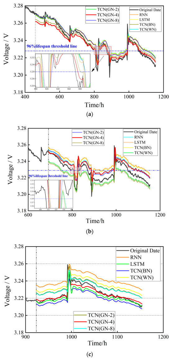
Figure 15.
Prediction results of multiple models for lifespan: (a) training set ratio of 40%; (b) training set ratio of 60%; (c) training set ratio of 80%.
Since the dataset did not reach the 90% lifespan failure threshold by the end of testing [43], a voltage lifespan threshold of 96% of the standard voltage value, i.e., 3.228 V, was adopted, The selection of this threshold avoids the early high noise interference corresponding to the 95% threshold, and fully utilizes the steady-state data in the 96–91% attenuation interval to reduce the uncertainty of extrapolation. In Figure 15a, the actual times when the voltage first and second reached the threshold were 807 h and 872 h, respectively. The EMD-TCN (GN-4) model predicted these times as 809 h and 876 h, respectively. In Figure 15b, the EMD-TCN (GN-4) model predicted the threshold-reaching times as 810 h and 886 h. Both prediction times were the closest to the actual values among all models, demonstrating that the model can accurately predict the steady-state lifespan of PEMFC.
Table 9.
Evaluation metrics of multiple model predictions: (a) Model prediction accuracy indicators; (b) Model prediction speed.
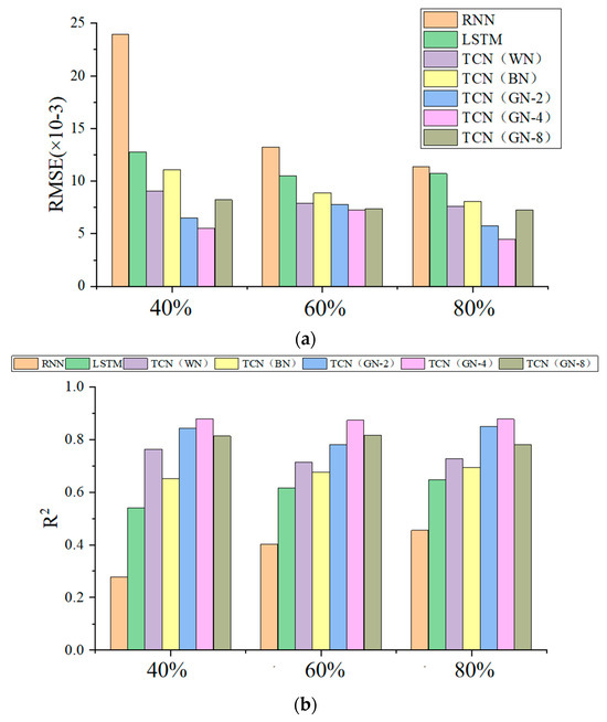
Figure 16.
Prediction results of multiple models. (a) comparison of RMSE results; (b) comparison of R2 results.
Analysis of the above figure and table shows the following:
(1) When the training set accounts for 40%, 60%, and 80% of the data respectively, the root mean square error (RMSE) value of the time convolutional network (TCN) (GN-4) prediction model based on empirical mode decomposition (EMD) is the smallest among the corresponding comparison groups. This indicates that the deviation between the predicted values and the actual values of this model is the smallest, thus demonstrating the best prediction performance. Its coefficient of determination (R2) value is also the highest in the same group, which means that this model can most effectively explain the variance of the voltage data and achieve the highest goodness-of-fit. Moreover, as the data volume increases, the RMSE shows a downward trend and R2 tends to be stable, indicating that the model has no risk of overfitting as the data volume increases. The dilated convolution structure of TCN can capture long-term time dependencies. Combined with the decomposition ability of EMD for non-stationary signals, the model can more accurately extract the core features of voltage attenuation when the data volume is sufficient.
(2) Comparative analysis shows that the time convolutional network (TCN) model based on empirical mode decomposition (EMD) significantly outperforms the traditional recurrent neural network (RNN) and long short-term memory network (LSTM) in prediction performance. When the training set data accounts for 40%, the root mean square error (RMSE) of the TCN (GN-4) model reaches 0.0055 V, a 76.96% reduction compared with the RNN baseline model (0.239 V). At the same time, its coefficient of determination (R2) increases to 0.879, a 217.3% increase compared with RNN (0.277), and the prediction accuracy and generalization ability are significantly improved. This confirms the powerful ability of EMD in extracting key information and its excellent adaptability to the analysis of nonlinear and non-stationary signals.
(3) A horizontal comparison of the prediction results of EMD-TCN (GN-4) under different training set ratios reveals that the fluctuation of the results is extremely small. This indicates that the TCN (GN) model has excellent learning ability, enabling it to effectively learn data features from a small dataset and make accurate predictions. There are no problems such as overfitting when the data volume increases, showing strong robustness to the data volume.
(4) Research on normalization methods shows that the group normalization TCN model can more accurately share statistical information, reducing the risk of overfitting, and significantly outperforms batch normalization, weight normalization, and traditional neural network models in terms of generalization ability. Under different training set sizes, the two evaluation indicators of group normalization, R2 and RMSE, perform well. Further research on the number of channels reveals that the model accuracy is highest when the number of channels is 4. The main reason is that when the data volume is small, using a smaller grouping parameter will result in a larger variance, and the calculation amount of the mean and variance is small, so the normalization effect is not as good as that of a larger grouping parameter. However, an excessively large grouping parameter will cause gradient competition among too many groups of parameters during back-propagation, leading to training instability and thus reducing the prediction accuracy
In recent years, models based on the Transformer architecture or the attention mechanism have also received widespread attention. By comparing the latest research results, this study shows that the proposed EMD-TCN(GN) model has significant advantages in terms of prediction accuracy and engineering applicability. The RMSE value of the RCLMA model (integrating residual convolution blocks, LSTM units, and multi-head self-attention layers) developed by scholars such as Sun [44] on the same test dataset is 0.01785, which is significantly higher than 0.00447 of this study; Although the transfer learning-Transformer hybrid model proposed by the Tang [45] team has a better scene transfer ability (it only needs to fine-tune parameters to adapt to different prediction scenarios), its RMSE value of 0.00598 is still 34.3% higher than that of this model. In general, the EMD-TCN(GN) model can extract features from each IMF component and residual of empirical mode decomposition, expanding the data dimension, and the model can train and learn feature information more effectively. The real-time state update mechanism accurately captures the reversible voltage recovery effect, overcoming the over-simplification defect of the life prediction model listed in the introduction. And compared with the Transformer model or the attention mechanism, its computational efficiency is higher, saves computing power, and is more convenient for embedded deployment, and the effect of the Transformer highly depends on high-quality historical data. If the data have noise or are missing, it may affect the prediction accuracy of the model, so a more complex data preprocessing process is required.
In order to deeply explore the prediction accuracy and model generalization of the EMD-TCN model in different prediction scenarios, the team introduces a new dataset for prediction. The data come from the cumulative results of 96 CLTC cycle working conditions on the 60 kW fuel cell test platform in the laboratory (as shown in Figure 17). If all the data are used for life prediction, it is very easy to have a gradient explosion and a huge amount of calculation, and the feasibility is low. Therefore, the high-speed interval data that have a greater impact on the performance degradation of the PEMFC is selected for prediction, and a total of 20,784 data points are screened out. On this basis, the equidistant window is selected, and one group of high-speed interval voltage data are taken for every four groups of cycles, totaling 24 groups. The voltage values are combined into a continuous dataset according to the test sequence, and finally 5196 original voltage time-series data points are obtained. In the data preprocessing process, the EMD method is used to process the voltage data to obtain five IMF components and one residual (res.). Compared with the decomposition of three IMF components in the steady-state working condition, this is mainly because the quality of the original data in the dynamic working condition is poor; there are extremely complex noises and outliers, resulting in excessive decomposition times, and the results are not ideal, which may affect subsequent prediction. Since the calculation amount of the dynamic voltage dataset and the steady-state voltage dataset is similar, according to the previous conclusion, the improved TCN (GN-4) model is selected for prediction. At the same time, in order to verify the applicability of the EMD-TCN model to the prediction of dynamic working conditions, the prediction results of the RNN and LSTM models are compared. R2 and RMSE are mainly selected as the model evaluation indicators. These two indicators can accurately reflect the overall goodness-of-fit of the model and the average deviation between the predicted values and the actual values. The experimental environment configuration and the proportion of the training set are consistent with the previous ones. The final prediction results are shown in Table 10.
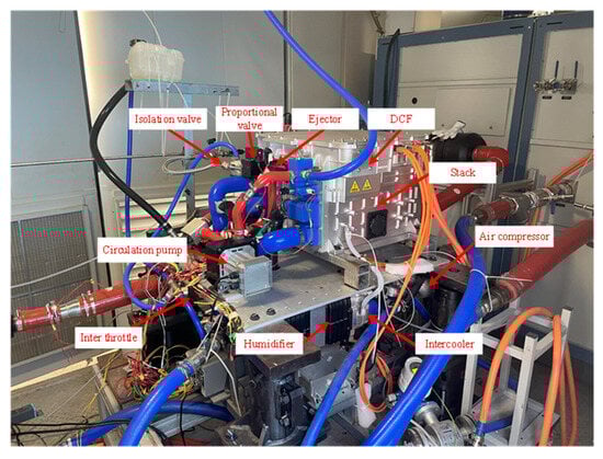
Figure 17.
The 60 kW fuel cell test bench [46].
Table 10.
RNN, LSTM, and EMD-TCN model prediction evaluation indicators.
Analysis shows that the EMD-TCN model achieves the highest R2 value of 0.712 and the lowest RMSE of 4.88 in predictions. These metrics are slightly worse than the steady-state prediction results under an 80% training set proportion (R2 = 0.877, RMSE = 4.47). This indicates that the discrepancies between predicted and actual values are relatively small under both dynamic and steady-state operating conditions, demonstrating strong prediction accuracy and robust model performance. However, the reduced R2 value suggests higher variability in predictions, implying that the model is sensitive to noise and outliers in dynamic scenarios. To address this, enhanced data preprocessing—such as incorporating unsupervised CGAN models for data reconstruction—should be prioritized in dynamic experiments to mitigate the impact of dataset biases and improve prediction stability.
5. Conclusions and Future Outlook
This paper proposes a PEMFC long-term lifespan prediction scheme based on EMD-TCN. The model consists of two identical internal convolution units and a residual connection structure. The logical sequence processed by a single convolution unit is as follows: causal convolution layer, normalization layer, activation function, and dropout layer. An in-depth study of the normalization layer was conducted. Compared to batch normalization and instance normalization, group normalization (GN) has lower computational complexity. Additionally, GN more accurately shares statistical information with fewer channels within a group, thereby reducing the risk of overfitting and improving the model’s generalization ability. To validate the model, the FCI dataset was first processed, then sliced and input into the model for prediction. RMSE and R2 were selected as evaluation metrics for prediction validation. The main conclusions are as follows:
The prediction results of RNN, LSTM, and TCN models were analyzed, and the prediction performance was found to be unsatisfactory, with the maximum R2 value only reaching 0.663. Therefore, an EMD-TCN prediction model was proposed, and its normalization layer was further analyzed. The RMSE of the TCN with group normalization (GN) was lower than that of TCN with weight normalization and batch normalization, and the R2 value was superior to those of the other two methods. This further demonstrates that TCN (GN) can accurately share statistical information within groups with fewer channels, reducing the risk of overfitting, and improving the model’s generalization ability. Moreover, further research on TCN group normalization features showed that appropriate grouped convolutions can increase the network’s nonlinear expression ability, reduce the number of parameters, and improve computational accuracy. The results indicated that for training set proportions of 40%, 60%, and 80%, the EMD-based TCN (GN-4) prediction model had the smallest RMSE value among the comparison groups, suggesting that the model’s predicted values were closest to the actual values and achieved the best prediction performance. Its R2 value was also the highest in the group, meaning the model explained the most variance in voltage data and had the best fit. For lifetime prediction, using a voltage threshold of 3.228 V (96% of the standard voltage value), the real values reached the threshold at 807 h and 872 h for the first and second times, respectively. The EMD-TCN (GN-4) model predicted the threshold reach times at 810 h and 886 h, respectively. This demonstrates that the model can accurately predict the lifetime of PEMFCs.
Compared to traditional RNN, LSTM, and TCN models, the proposed EMD-TCN model offers higher prediction accuracy. The in-depth study of its normalization layer reduces computational load, lowers overfitting risks, and enhances the model’s generalization ability. This research is significant for improving the accuracy, reliability, and stability of PEMFC lifetime prediction.
Although our study shows that EMD-TCN outperforms conventional models, it primarily demonstrates its precision in steady-state output conditions. In the future, we plan to apply it to different devices and more complex scenarios to improve computational speed and prediction accuracy, enabling more accurate lifetime predictions and faster fault diagnosis, thereby promoting the large-scale application of fuel cells.
Author Contributions
Conceptualization, C.Z., C.D., J.Z., Y.Z., J.S. and J.H.; methodology, C.Z., C.D., J.Z. and Y.Z.; software, C.Z., J.Z., Y.Z. and J.H.; validation, C.Z., J.Z., Y.Z. and J.H.; formal analysis, C.D. and J.S.; investigation, Y.Z. and C.Z.; resources, C.Z., C.D., Y.Z. and J.S.; data curation, C.Z., C.D., J.Z. and Y.Z.; writing—original draft preparation, C.Z., J.Z. and Y.Z.; writing—review and editing, C.Z., C.D., J.Z., J.S. and J.H.; visualization, C.Z., C.D., J.Z., Y.Z., J.S. and J.H.; supervision, C.D. and J.S.; project administration, C.D. and J.S.; funding acquisition, C.D. All authors have read and agreed to the published version of the manuscript.
Funding
This work was supported by the Foshan Xianhu Laboratory of the Advanced Energy Science and Technology Guangdong Laboratory (XHRD2024-11233100-01) and the Key R&D project of Hubei Province, China (2021AAA006).
Data Availability Statement
The dataset is available on request from the authors.
Conflicts of Interest
The author, Yiming Zhang, is an employee of Dongfeng Motor Corporation Research & Development Institute. The other authors declare no conflicts of interest.
References
- Jia, C.; He, H.; Zhou, J.; Li, J.; Wei, Z.; Li, K. Learning-based model predictive energy management for fuel cell hybrid electric bus with health-aware control. Appl. Energy 2024, 355, 122228. [Google Scholar] [CrossRef]
- Li, X.; Ye, T.; Meng, X.; He, D.; Li, L.; Song, K.; Jiang, J.; Sun, C. Advances in the Application of Sulfonated Poly(Ether Ether Ketone) (SPEEK) and Its Organic Composite Membranes for Proton Exchange Membrane Fuel Cells (PEMFCs). Polymers 2024, 16, 2840. [Google Scholar] [CrossRef] [PubMed]
- Alenazey, F.; Alyousef, Y.; AlOtaibi, B.; Almutairi, G.; Minakshi, M.; Cheng, C.K.; Vo, D.-V.N. Degradation Behaviors of Solid Oxide Fuel Cell Stacks in Steady-State and Cycling Conditions. Energy Fuels 2020, 34, 14864–14873. [Google Scholar] [CrossRef]
- Hua, Z.; Zheng, Z.; Pahon, E.; Péra, M.-C.; Gao, F. A review on lifetime pre-diction of proton exchange membrane fuel cells system. J. Power Sources 2022, 529, 231256. [Google Scholar] [CrossRef]
- Jia, C.; He, H.; Zhou, J.; Li, K.; Li, J.; Wei, Z. A performance degradation prediction model for PEMFC based on bi-directional long short-term memory and multi-head self-attention mechanism. Int. J. Hydrogen Energy 2024, 60, 133–146. [Google Scholar] [CrossRef]
- Zhou, D.; Wu, Y.; Gao, F.; Breaz, E.; Ravey, A.; Miraoui, A. Degradation Prediction of PEM Fuel Cell Stack Based on Multi-Physical Aging Model with Particle Filter Approach. IEEE Trans. Ind. Appl. 2017, 53, 4041–4042. [Google Scholar] [CrossRef]
- Hu, Z. Research on Durability Modeling and State Estimation of Automotive Fuel Cell Systems; Tsinghua University: Beijing, China, 2019; p. 33. [Google Scholar]
- Bressel, M.; Hilairet, M.; Hissel, D.; Bouamama, B.O. Extended Kalman Filter for prognostic of Proton Exchange Membrane Fuel Cell. Appl. Energy 2016, 164, 220–227. [Google Scholar] [CrossRef]
- Sharaf, O.Z.; Orhan, M.F. An overview of fuel cell technology: Fundamentals and applications. Renew. Sustain. Energy Rev. 2014, 32, 810–853. [Google Scholar] [CrossRef]
- Jouin, M.; Gouriveau, R.; Hissel, D.; Péra, M.-C.; Zerhouni, N. Degradations analysis and modeling for health assessment and prognostics of PEMFC. Raliability Eng. Syst. Saf. 2016, 148, 78–95. [Google Scholar] [CrossRef]
- Zhang, D.; Cadet, C.; Yousfi-Steiner, N. Some improvments of Particle Filtering Based Prognosis for PEM Fuel Cell. IFAC-PapersOnline 2016, 49, 162–167. [Google Scholar] [CrossRef]
- Zhang, J.; Yan, F.; Du, C.; Zhang, Y.; Zheng, C.; Wang, J.; Chen, B. A Multi-Feature Fusion Method for Life Prediction of Automotive Proton Exchange Membrane Fuel Cell Based on TCN-GRU. Materials 2024, 17, 4713. [Google Scholar] [CrossRef] [PubMed]
- Liu, J. Research on Data-Driven Fault Diagnosis and Life Prediction Methods for PEMFC Power Generation Systems; Southwest Jiaotong University: Chengdu, China, 2020. [Google Scholar]
- Lv, J.; Yu, Z.; Zhang, H.; Sun, G.; Muhl, P.; Liu, J. Transformer Based Long-Term Prognostics for Dynamic Operating PEM Fuel Cells. IEEE Trans. Transp. Electrif. 2024, 10, 1747–1757. [Google Scholar] [CrossRef]
- Zhou, J.; Zhang, J.; Yi, F.; Feng, C.; Wu, G.; Li, Y.; Zhang, C.; Wang, C. A real-time prediction method for PEMFC life under actual operating conditions. Sustain. Energy Technol. Assess. 2024, 70, 103949. [Google Scholar] [CrossRef]
- Kethaki Pabasara Wickramaarachchi, W.A.M.; Minakshi, M.; Gao, X.; Dabare, R.; Wong, K.W. Hierarchical porous carbon from mango seed husk for electro-chemical energy storage. Chem. Eng. J. Adv. 2021, 8, 100158. [Google Scholar] [CrossRef]
- Wu, Y.; Breaz, E.; Gao, F.; Miraoui, A. A modified relevance vector machine for PEM fuel-cell stack aging prediction. IEEE Trans. Ind. Appl. 2016, 52, 2573–2581. [Google Scholar] [CrossRef]
- Morando, S.; Jemei, S.; Gourivrau, R.; Zerhouni, N.; Hissel, D. Fuel Cells Remaining Useful Lifetime forecasting using Echo State Network. In Proceeding of the IEEE Vehicle Power and Propulsion Conference, Coimbra, Portugal, 27–30 October 2014. [Google Scholar]
- Li, L.; Zhao, Z.; Zhao, X.; Lin, K.-Y. Gated recurrent unit networks for remaininguseful life prediction. IFAC-PapersOnLine 2020, 53, 10498–10504. [Google Scholar] [CrossRef]
- He, K.; Liu, Z.; Sun, Y.; Mao, L.; Lu, S. Degradation prediction of proton exchange membrane fuel cell using auto-encoder based health indicator and long short-term memory network. Int. J. Hydrogen Energy 2022, 47, 35055–35067. [Google Scholar] [CrossRef]
- Yi, F.; Shu, X.; Zhou, J.; Zhang, J.; Feng, C.; Gong, H.; Zhang, C.; Yu, W. Remaining useful life prediction of PEMFC based on matrix long short-term memory. Int. J. Hydrogen Energy 2025, 111, 228–237. [Google Scholar] [CrossRef]
- Zhou, J.; Shu, X.; Zhang, J.; Yi, F.; Jia, C.; Zhang, C.; Kong, X.; Zhang, J.; Wu, G. A deep learning method based on CNN-BiGRU and attention mechanism for proton exchange membrane fuel cell performance degradation prediction. Int. J. Hydrogen Energy 2024, 94, 394–405. [Google Scholar] [CrossRef]
- Mao, L.; Jackson, L. Selection of optimal sensors for predicting performance of polymer electrolyte membrane fuel cell. J. Power Sources 2016, 328, 151–160. [Google Scholar] [CrossRef]
- Zhu, W.; Guo, B.; Li, Y.; Yang, Y.; Xie, C.; Jin, J.; Gooi, H.B. Uncertainty quantification of proton-exchange-membrane fuel cells degradation prediction based on Bayesian-Gated Recurrent Unit. eTransportation 2023, 16, 100230. [Google Scholar] [CrossRef]
- Li, Q.; Gao, Z. A Similarity-based prognostics approach for full cells state of health. In Proceeding of the Prognostics and System Health Management Conference, Zhangjiajie, China, 28–31 May 2024. [Google Scholar]
- IEEE PHM Society. “PHM 2014 Data Challenge Dataset”, 2014. Available online: https://search-data.ubfc.fr/FR-18008901306731-2021-07-19_IEEE-PHM-Data-Challenge-2014.html (accessed on 25 May 2025).
- Chen, K.; Laghrouche, S.; Djerdir, A. Degradation prediction of proton exchange membrane fuel cell based on grey neural model and particle swarm optimization. Energy Convers. Manag. 2019, 195, 810–818. [Google Scholar] [CrossRef]
- Cheng, J.; Yu, D.; Yang, Y. Research on the intrinsic mode function (IMF) criterion in EMD method. Mech. Syst. Signal Process. 2006, 20, 817–824. [Google Scholar]
- Pang, H.; Gao, F.; Cheng, G.; Luo, H.; Chen, J.; Wen, Y. Time-of-use modeling and prediction of daily power transmission based on empirical mode decomposition and extreme learning machine. Smart Power 2021, 49, 63–69. [Google Scholar]
- Li, P. Life Prediction Technology of Hydrogen Fuel Cell Based on Cyclic Neural Network; University of Electronic Science and Technology of China: Chengdu, China, 2021. [Google Scholar]
- Salva, J.A.; Iranzo, A.; Rosa, F.; Tapia, E.; Lopez, E.; Isorna, F. Optimization of a PEM fuel cell operating conditions: Obtaining the maximum performance polarization curve. Int. J. Hydrogen Energy 2016, 41, 19713–19723. [Google Scholar] [CrossRef]
- Wu, Y.; Yuan, M.; Dong, S.; Lin, L.; Liu, Y. Remaining useful life estimation of engineered systems using vanilla LSTM neural networks. Neurocomputing 2018, 275, 167–179. [Google Scholar] [CrossRef]
- Liu, J.; Li, Q.; Chen, W.; Yan, Y.; Qiu, Y.; Cao, T. Remaining useful life prediction of PEMFC based on long short-term memory recurrent neural networks. Int. J. Hydrogen Energy 2019, 44, 5470–5480. [Google Scholar] [CrossRef]
- Xu, S.; Niu, R. Displacement prediction of Baijiabao landslide based on empirical mode decomposition and long short-term memory neural network in Three Gorges area, China. Comput. Geosci. 2018, 111, 87–96. [Google Scholar] [CrossRef]
- Cabrera, D.; Guamán, A.; Zhang, S.; Cerrada, M.; Sánchez, R.-V.; Cevallos, J.; Long, J.; Li, C. Bayesian approach and time series dimensionality reduction to LSTM-based model-building for fault diagnosis of a reciprocating compressor. Neurocomputing 2020, 380, 51–66. [Google Scholar] [CrossRef]
- Zuo, B.; Cheng, J.; Zhang, Z. Degradation prediction model for proton exchange membrane fuel cells based on long short-term memory neural network and Savitzky-Golay filter. Int. J. Hydrogen Energy 2021, 46, 15928–15937. [Google Scholar] [CrossRef]
- Pei, P.; Chen, H. Main factors affecting the lifetime of Proton Exchange Membrane fuel cells in vehicle applications: A review. Appl. Energy 2014, 125, 60–75. [Google Scholar] [CrossRef]
- Ulyanov, D.; Vedaldi, A.; Lempitsky, V. Improved Texture Networks: Maximizing Quality and Diversity in Feed-Forward Stylization and Texture Synthesis. In Proceedings of the 2017 IEEE Conference on Computer Vision and Pattern Recognition (CVPR), Honolulu, HI, USA, 21–26 July 2017; pp. 4105–4113. [Google Scholar]
- Tu, C.; Zhou, F.; Pan, M. A model with high-precision on proton exchange membrane fuel cell performance degradation prediction based on temporal convolutional network-long short-term memory. Int. J. Hydrogen Energy 2024, 74, 414–422. [Google Scholar] [CrossRef]
- Zhang, F.; Shen, Z.; Xu, M.; Xie, Q.; Fu, Q.; Ma, R. Remaining useful life prediction of lithium-ion batteries based on TCN-DCN fusion model combined with IRRS filtering. J. Energy Storage 2023, 72 Part D, 108586. [Google Scholar] [CrossRef]
- Nguyen, K.T.P.; Medjaher, K. A new dynamic predictive maintenance framework using deep learning for failure prognostics. Reliab. Eng. Syst. Saf. 2019, 188, 251–262. [Google Scholar] [CrossRef]
- Li, Z.; Outbib, R.; Hissel, D.; Giurgea, S. Data-driven diagnosis of PEM fuel cell: A comparative study. Control Eng. Pract. 2014, 28, 1–12. [Google Scholar] [CrossRef]
- Ma, R.; Yang, T.; Breaz, E.; Li, Z.; Briois, P.; Gao, F. Data-driven proton exchange membrane fuel cell degradation predication through deep learning method. Appl. Energy 2018, 231, 102–115. [Google Scholar] [CrossRef]
- Sun, X.; Xie, M.; Fu, J.; Zhou, F.; Liu, J. An improved neural network model for predicting the remaining useful life of proton exchange membrane fuel cells. Int. J. Hydrogen Energy 2023, 48, 25499–25511. [Google Scholar] [CrossRef]
- Tang, X.; Qin, X.; Wei, K.; Xu, S. A novel online degradation model for proton exchange membrane fuel cell based on online transfer learning. Hydrog. Energy 2023, 48, 13617–13632. [Google Scholar] [CrossRef]
- Li, X.; Wei, H.; Du, C.; Shi, C.; Zhang, J. Control strategy for the anode gas supply system in a proton exchange membrane fuel cell system. Energy Rep. 2023, 10, 4342–4358. [Google Scholar] [CrossRef]
Disclaimer/Publisher’s Note: The statements, opinions and data contained in all publications are solely those of the individual author(s) and contributor(s) and not of MDPI and/or the editor(s). MDPI and/or the editor(s) disclaim responsibility for any injury to people or property resulting from any ideas, methods, instructions or products referred to in the content. |
© 2025 by the authors. Licensee MDPI, Basel, Switzerland. This article is an open access article distributed under the terms and conditions of the Creative Commons Attribution (CC BY) license (https://creativecommons.org/licenses/by/4.0/).