The Effect of Domain Length and Initialization Noise on Direct Numerical Simulation of Shear Stratified Turbulence

Abstract

Direct numerical simulation (DNS) has been employed with success in a variety of oceanographic applications, particularly for investigating the internal dynamics of Kelvin–Helmholtz (KH) billows. However, it is difficult to relate these results directly with observations of ocean turbulence due to the significant scale differences involved (ocean shear layers are typically on the order of tens to hundreds of meters in thickness, compared to DNS studies, with layers on the order of one to tens of centimeters). As efforts continue to inform our understanding of geophysical-scale turbulence by extrapolating DNS results, it is important to understand the impact of model setup and initial conditions on the resulting turbulent quantities. Given that geophysical-scale measurements, whether through microstructures or other techniques, can only provide estimates of averaged TKE quantities (e.g., TKE dissipation or buoyancy flux), it may be necessary to compare mean turbulent quantities derived from DNS (i.e., across one or more complete billow evolutions) with ocean measurements. In this study, we analyze the effect of domain length and initial velocity noise on resulting turbulent quantities. Domain length is important, as dimensions that are not integer multiples of the natural KH billow wavelength may compress or stretch the billows and impact their energetics. The addition of random noise in the initial velocity field is often used to trigger turbulence and suppress secondary instabilities; however, the impact of noise on the resulting turbulent energetics is largely unknown. In this study, we conclude that domain lengths on the order of 1.5 times the natural wavelength or less can affect the resulting turbulent energetics by a factor of two or more. We also conclude that increasing the amplitude of random initial velocity noise decreases the resulting turbulent energetics, but that different realizations of the random noise field may have an even greater impact than amplitude. These results should be considered when designing a DNS experiment.

1. Introduction

The transition of stratified shear flow to turbulence is one of the classical problems of fluid mechanics and is often attributed to processes driven by Kelvin–Helmholtz or similar instabilities [1,2,3]. Kelvin–Helmholtz (K-H) billow formation and its resulting instabilities have been extensively studied in the laboratory [4,5], in field observations [6,7,8], through theoretical methods [9,10], and, recently, by high-resolution numerical simulations [11,12,13].

Typically, field observations cannot provide a comprehensive assessment of the formation and evolution of K-H billows (e.g., [14,15]). There have been analytical studies to define billow structure, but these have been unable to result in stable solutions [16,17,18]. Recently, with increasing computational power, 3D models of K-H instabilities have been used to evaluate K-H evolution and the resulting changes in density and velocity profiles [12,19,20].

1.1. Stratified Shear Turbulence

The Reynolds and Richardson numbers are two important parameters to characterize stratified shear flow. The Reynolds number is expressed as $Re={\displaystyle \frac{u_0{h}_0}{\nu }}$, where $u_0$ is the velocity difference between two layers, $h_0$ is the shear layer thickness, and $\nu$ is the kinematic viscosity. The Reynolds number represents the relative strength of inertial forces to viscous forces.

The Richardson number $Ri$ is defined as $Ri={\displaystyle \frac{g\mathsf{\Delta }\rho h_0}{{\rho }_0{u}_0^2}}$, where g is gravity, $\mathsf{\Delta }\rho$ is the difference in density between two flowing layers, and ${\rho }_0$ is the density of the heavier fluid. The Richardson number represents the stability of the flow, with $Ri<{\displaystyle \frac{1}{4}}$ a necessary condition for velocity shear to overcome stratification and generate turbulence [21,22]. If $Ri$ is large, it usually suppresses turbulent mixing [23].

Within a numerical domain utilizing periodic boundary conditions in x and y and no-flux boundaries in z, terms representing the transport of turbulent kinetic energy (TKE) are equal to zero when averaged over the whole domain. Then, the TKE equation for a homogeneous turbulent field becomes [24]:

$${\displaystyle \frac{dE}{dt}}=P-B-ϵ$$

(1)

where P is the shear production of TKE, B is the buoyancy flux, and $ϵ$ is the dissipation rate (the reader is referred to [25] for additional information on the equations presented here, including their derivation). Here, P is given by

$$P=-\overline{u^{\prime }{w}^{\prime }}{\displaystyle \frac{\partial \overline{u}}{\partial z}}$$

(2)

where primes represent fluctuations from the horizontal mean. To evaluate the terms in Equation (1) we use the spatial means.

Over most time scales, the momentum flux $\overline{u^{\prime }{w}^{\prime }}$ is, by definition, of opposite sign of the mean shear, resulting in a positive contribution to the TKE, although recent DNS studies [26] have shown that production can briefly act as a sink of TKE (i.e., forcing the mean flow) during Kelvin–Helmholtz evolution.

The buoyancy flux can be a source or sink term depending on the sign of $\overline{w^{\prime }{\rho }^{\prime }}$. In most stable stratified fluids, B is negative and acts as a sink of TKE over longer timescales; however, the sign may fluctuate during K-H evolution depending on the phase of billow development and during brief periods of unstable stratification during billow roll-up. Buoyancy flux is given by

$$B=-{\displaystyle \frac{g}{{\rho }_0}}\overline{w^{\prime }{\rho }^{\prime }}$$

(3)

The viscous dissipation $\epsilon$ is the conversion of TKE into heat. This process occurs at the smallest turbulence scales, known as the Kolmogorov length scales: $\eta ={({\nu }^3/ϵ)}^{1/4}$. Here, $ϵ$ is the average rate of dissipation of turbulence kinetic energy per unit mass.

$$ϵ=-2\nu \overline{e_{ij}{e}_{ij}}$$

(4)

where $e_{ij}={\displaystyle \frac{1}{2}}({\displaystyle \frac{\partial u_i^{\prime }}{\partial x_j}}+{\displaystyle \frac{\partial u_j^{\prime }}{\partial x_i}})$

Given the need for spatial resolution approaching the Kolmogorov scales, the overall domain size of most DNS runs must be constrained to meet computational limits: generally constraining DNS runs to low-$Re$ flows, consistent with laboratory scales.

1.2. Direct Numerical Simulation (DNS) Solution

Turbulence is an extremely complex system, with no satisfying analytical solution for even the simplest turbulent flows. It must be numerically solved by a solution of Navier–Stokes equations at small scales or parameterized in larger-scale ocean models, e.g., [27]. In recent years, with significant computational advancement, DNS solutions to turbulent flows have become available for some problems. In DNS, the smallest spatial and temporal scales of turbulence, i.e., the energy dissipating or Kolmogorov scales, are resolved, and with increasing computational power, it may be possible to solve higher-$Re$ flows.

Although many studies have been successful at obtaining DNS solutions to stratified turbulent flows relevant to the ocean, e.g., [11,12,28,29,30,31,32,33,34], the $Re$ is relatively low compared to typical oceanic values of ${10}^6$ to ${10}^7$. Even the high-$Re$ flows in the DNS literature are still on the order of ${10}^4$ and thus are not much beyond the typical realm of laboratory flows [35]. The scales associated with typical oceanic turbulent flows are extremely difficult, if not impossible, to resolve in DNS runs due to computational limitations. Nevertheless, there are important considerations when setting up DNS runs for such applications, including initial and boundary conditions, including the introduction of noise, which are discussed next.

1.2.1. Initial and Boundary Conditions

The domain size and spatial resolution of a DNS run depend on the largest and smallest scales that need to be resolved. Resolution should be capable of representing the Kolmogorov length scale, while the numerical timestep should resolve the Kolmogorov time scale, $\tau ={\left({\displaystyle \frac{\nu }{ϵ}}\right)}^{1/2}$. Initial conditions such as the mean flow velocity profiles, mean density profiles, and other flow characteristics are important parameters that may have a significant impact on the overall simulation. Some researchers also use initial noise or a perturbation velocity in their simulations.

Different initial conditions, including the magnitude of “noise” imposed on the initial velocity field, as well as the overall domain length can change the resulting turbulent quantities: P, B, and $\epsilon$. However, the detailed impact of these initial conditions has not yet been investigated.

1.2.2. Previous DNS Efforts and Utilization of Noise

In many cases, previous studies have included an initial noise field or perturbation [36] to trigger the generation of overturns and suppress secondary instabilities, which can help the Kelvin–Helmholtz billow to transition to fully developed turbulence [37]. This noise is typically added to the initial velocity field, but the impact of the noise on the final turbulent quantities has not been fully investigated.

Smyth [11] added a vorticity perturbation to the initial conditions to simulate primary and pairing instabilities. The growth of secondary vortices on braids of separating Kelvin–Helmholtz billows was investigated. The Reynolds number was varied from 1000 to 6000, while the Richardson number was varied from 0.04 to 0.16. To obtain fully turbulent flow, a perturbation was also added to the streamwise velocity in [36]. Their results suggest that the small-scale structure is independent of the initial or boundary conditions. The impact of perturbation intensity was more recently investigated by Kaminski and Smyth [38], who found a marked decrease in turbulence generation and less clearly defined billows for large-amplitude perturbations.

To excite three-dimensional secondary instabilities, a cross-sectional velocity was added as random noise in [39]. Here, DNS was used with $Re$ values ranging from 1500 to 5000 and $R{i}_B$ values from 0.08 to 0.16 to model ocean stratified-shear-flow-induced turbulence resulting from a pair of unstable Kelvin–Helmholtz-induced billows.

A wide variety of secondary instabilities have been investigated using DNS [12]. In these simulations, incompressible white noise is added to the velocity and white noise of zero mean is added to the density. Caulfield and Peltier [40] used a perturbation in their simulations, which was imposed on the background flow, and a small-amplitude isotropic noise field was applied to the streamwise velocity in the initialization, with $Re=750$ and $R{i}_B$ ranging from 0 to 0.1. Despite the wide application of initial conditions such as noise, little effort has been made to quantify the effect of these parameters on the resulting turbulence.

1.2.3. Oceanographic Implications

To date, DNS has been employed with limited success for oceanographic applications. Most DNS studies, such as those discussed above, have focused on the internal dynamics of turbulence, and it is often difficult to relate these results directly to observations of ocean turbulence. Given the vast scale difference and the inability to observe individual billows in the field with sufficient detail, comparisons of averaged turbulent quantities would be the primary approach to compare DNS results with field data. As noted above, many previous studies use initial perturbations or noise or a combination of both to excite turbulence or suppress secondary instabilities.

In addition, DNS studies often utilize a fixed domain length (x-direction), which is typically established by approximation of the natural K-H billow wavelength but is sometimes compressed to reduce the domain size and computational time. Due to the standard assumption of periodicity in the streamwise direction, an arbitrary domain length may have the unintended effect of compressing or stretching the natural wavelength of resulting K-H billows, which may significantly impact their energetics, particularly in a domain-averaged sense. Adding additional energy in the form of noise may also significantly change the mean turbulent quantities. Identifying the impact of these initial choices is essential for the application of future DNS research attempting to extrapolate overall turbulence quantities to larger scales and to enable stronger connections between DNS and observations. In this study, we investigate the impact of varying both domain length and initial noise in the velocity field.

In Section 2, the model setup is presented with a description of initial and boundary conditions. The approach for varying the domain length and noise amplitude is also explained. In Section 3, we present the impacts of domain length on the formation of billows, their wavelengths, and the resulting turbulence. Section 4 is focused on the noise analysis and is presented in two parts: one focusing on varying noise amplitude using a constant random field and the other on the impact of different random fields using a constant amplitude. Section 5 concludes with a brief discussion and summary.

2. Governing Equations and Numerical Methods

The DNS results were obtained using the NGA flow solver [41], which solves the variable density, low Mach number Naiver–Stokes equations. The governing equations include conservation of mass:

$${\displaystyle \frac{\partial \rho }{\partial t}}+\nabla ·\left(\rho \mathbf{u}\right)=0$$

(5)

and conservation of momentum:

$${\displaystyle \frac{\partial \left(\rho \mathbf{u}\right)}{\partial t}}+\nabla ·\left(\rho \mathbf{u}\mathbf{u}\right)=-\nabla p+\nabla ·\sigma +\rho \mathbf{g}$$

(6)

where p is the pressure, $\mathbf{g}$ is the gravitational acceleration, and $\sigma$ is the stress tensor given by

$$\sigma =\mu \left(\nabla \mathbf{u}+{\nabla }^T\mathbf{u}\right)-{\displaystyle \frac{2}{3}}\nabla ·\left(\mathbf{uI}\right)$$

(7)

Here, $\mu$ is the dynamic viscosity, and $\mathbf{I}$ is the identity tensor.

Density is determined from a conserved scalar Z that represents mixing, which is governed by the following transport equation:

$${\displaystyle \frac{\partial \left(\rho Z\right)}{\partial t}}+\nabla ·\left(\rho \mathbf{u}Z\right)=\nabla ·\left(\rho D_Z\nabla Z\right)$$

(8)

where $D_Z$ denotes the diffusivity coefficient.

The numerical methods of NGA have been detailed in [41] and are only briefly described here: Time advancement is done by the semi-implicit second-order Crank–Nicolson scheme of Pierce and Moin [42]. Using the classical fractional step approach [43], this iterative time advancement scheme uses staggering in time between the momentum field and the scalar (including density) fields. The scalars are advanced first, the density field is updated, and the momentum equation is then advanced [41]. A combination of a spectral method and Krylov-based methods [44] is used to solve the pressure Poisson equation. For numerical stability, the timestep $\mathsf{\Delta }t$ is constrained by various restrictions, including the Courant–Friedrichs–Lewy (CFL) condition applied to explicit numerical schemes [45]. The CFL condition requires the maximum of ${\displaystyle \frac{u\mathsf{\Delta }t}{\mathsf{\Delta }x}}$, ${\displaystyle \frac{v\mathsf{\Delta }t}{\mathsf{\Delta }y}}$, ${\displaystyle \frac{w\mathsf{\Delta }t}{\mathsf{\Delta }z}}$ to be less than unity, where $\mathsf{\Delta }x,\mathsf{\Delta }y,\mathsf{\Delta }z$ denote the grid size in each direction.

Figure 1 shows an example domain and an initial density profile. Here, x is the streamwise direction, y is the lateral direction, and z is the vertical direction aligned with gravity. The lengths of the domain in the x, y, and z directions are $L_x$, $L_y$, and $L_z$. We used various $L_x$ values in our simulations, while $L_y$ and $L_z$ were held constant. The number of grid points in the x-direction varied from 200 to 1104, and there were 64 and 256 grid points in the y- and z-directions, respectively. The grid resolution is reported in Table 1. At $z=0$ and $z=L_z$ of the 3D domain, an impermeable free slip condition is applied. The boundaries at $x=0$ and $x=L_x$ are periodic.

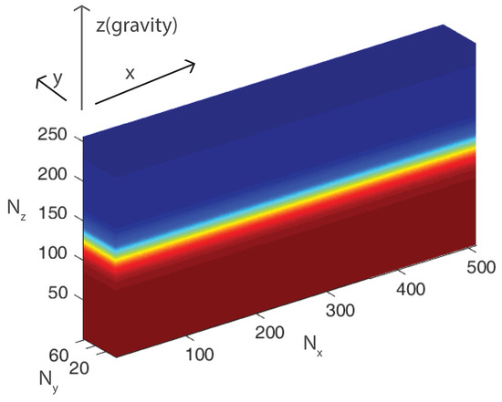
Figure 1. The 3D domain of the density field shown for $Lx=5.24$ m, $L_y=0.64$ m, and $L_z=2.62$ m.

Table 1. Main parameters used in the domain length analysis runs, with $Re=3610,Ri=0.12,L_y=0.64$ m, and $L_z$ = 2.62 m.

${\mathit{L}}_{\mathit{x}}\left(\mathit{m}\right)$	$\frac{{\mathit{L}}_{\mathit{x}}}{{\mathit{L}}_{\mathit{KH}}}$	$\frac{{\mathit{L}}_{\mathit{x}}}{{\mathit{L}}_{\mathit{KH}}^{*}}$	${\mathit{N}}_{\mathit{x}}$	$\mathsf{\Delta }\mathit{x}\left(\mathit{m}\right)$
2	0.67	0.40	200	0.01
2.49	0.84	0.50	256	0.0097
3.25	1.09	0.65	318	0.0102
3.98	1.33	0.80	392	0.0101
4.22	1.42	0.85	416	0.0101
4.48	1.50	0.90	448	0.01
4.97	1.67	1.00	488	0.0102
5.24	1.76	1.05	512	0.0102
6.21	2.08	1.25	600	0.0104
7.46	2.50	1.50	736	0.0101
8.7	2.92	1.75	848	0.0103
9.94	3.33	2.00	968	0.0103
11.18	3.75	2.25	1104	0.0101

The initial conditions were adopted from [36], with the major difference being that no perturbation was used here. The following initial velocity profile was imposed:

$$\overline{u}\left(z\right)={\displaystyle \frac{u_0}{2}}\tanh {\displaystyle \frac{2z}{h_0}}$$

(9)

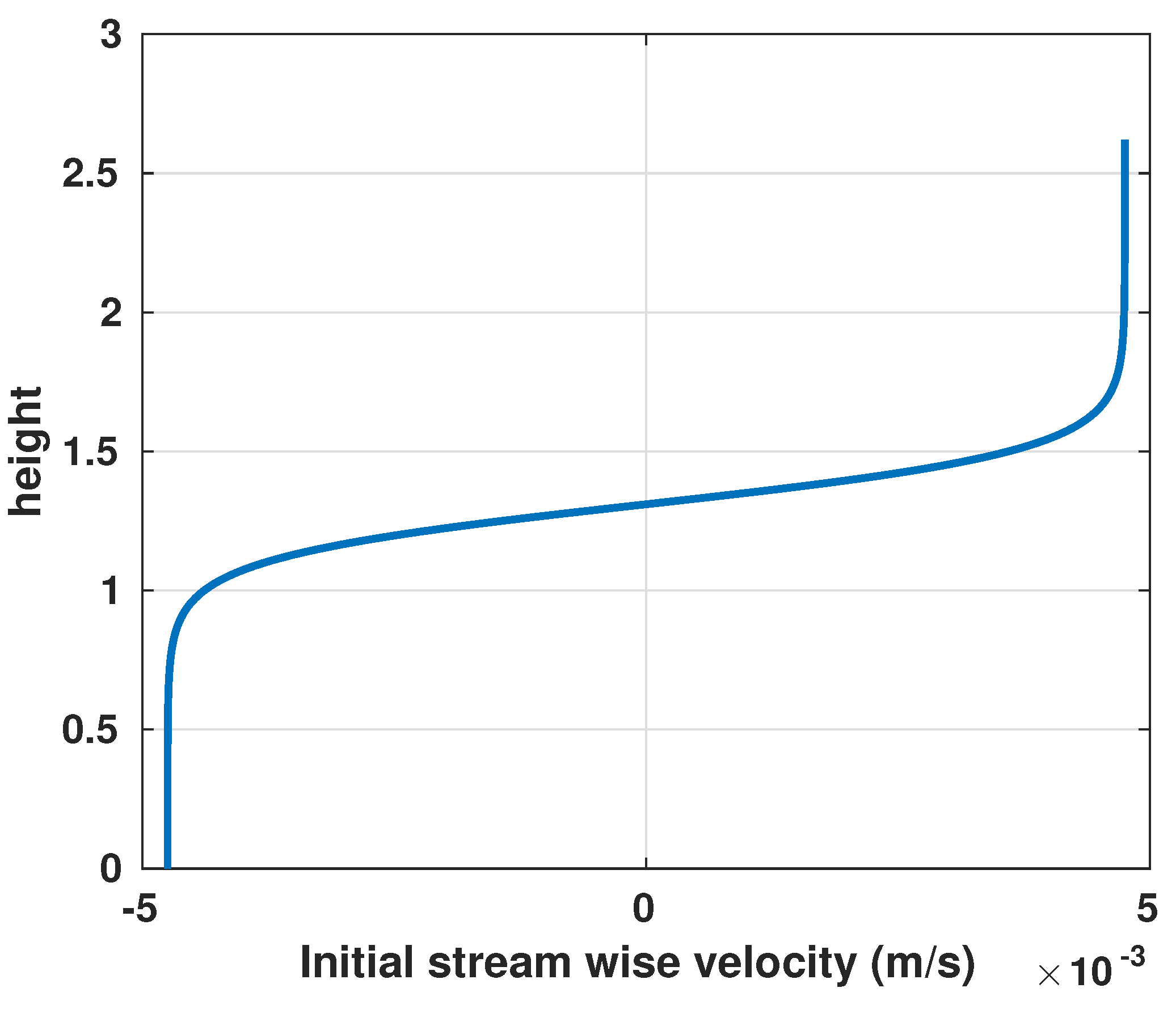
and $\overline{v}=\overline{w}=0$ Here, $h_0$ is the shear layer thickness, and $u_0$ is the magnitude of the velocity difference between the layers. In this study, $u_0$ is held constant at $u_0=0.0095$ m/s, and $h_0=0.38$ m for all simulations, which means $\overline{u}\left(z\right)$ varies from $-u_0/2$ to $u_0/2$, as shown in Figure 2.

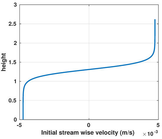
Figure 2. Representative initial velocity profile for DNS runs.

The initial density profile $\overline{\rho }\left(z\right)$ is prescribed by the following expression:

$$\overline{\rho }\left(z\right)={\rho }_0-{\displaystyle \frac{\mathsf{\Delta }\rho }{2}}(1+\tanh {\displaystyle \frac{2z}{h_0}})$$

(10)

where ${\rho }_0=999.69$ kg/m³ is regarded as the reference density, and $\mathsf{\Delta }\rho =0.0029$ kg/m³ is the density difference between $z=0$ and $z=L_z$. Furthermore, in this study, $g=9.81$ m/s² and $\mu =$ 0.001 Pa·s. Using these values, the Reynolds number ($Re={\displaystyle \frac{u_0{h}_0}{\nu }}$) and the Richardson number ($Ri={\displaystyle \frac{g\mathsf{\Delta }\rho h_0}{{\rho }_0{u}_0^2}}$) are calculated and held constant at $Re=3610$ and $Ri=0.12$ to maintain the same stability conditions.

To evaluate turbulent parameters at any particular instance in time, the total three-dimensional flow field is considered. We begin by averaging the 3D velocity field $\mathbf{u}$ on the horizontal x-y plane across the entire domain, resulting in mean vertical profiles of velocity that vary with time. The three-dimensional fluctuation to this z-dependent averaged field can be calculated by subtracting $\overline{U}(z,t),\overline{V}(z,t),\overline{W}(z,t)$ from the velocity field and applying Equations (2)–(4).

Then, P, B, and $\epsilon$ can be averaged in all three dimensions to obtain time-dependent instantaneous turbulent quantities, e.g., $P\left(t\right)=<P(x,y,z,t){>}_{xyz}$. We also integrate these values $\left(P\right(t),B(t),\epsilon (t\left)\right)$ over time to quantify the cumulative amount of work done by turbulence production, mixing, and dissipation.

One of our primary goals is to find the effect of random noise on final turbulent quantities. To do this, a random field $r_v(x,y,z)$ is used to set the initial condition for cross-stream velocity $\left(v\right)$:

$$\tilde{v}(x,y,z)=a{\displaystyle \frac{u_0}{2}}{r}_v(x,y,z){\mathrm{sech}}^2{\displaystyle \frac{2z}{h_0}}$$

(11)

Here, a is the amplitude of the noise, which is varied from 0 to 0.05 in our simulations, and $r_v(x,y,z)$ is the random function, which is uniformly distributed from −1 to 1 (Figure 3a). Although a normal (or Gaussian) distribution may be more effective at representing naturally occurring noise, a uniform distribution is used here, following [39]. In the variable-amplitude part of the noise analysis, $r_v$ is held constant for multiple simulations, with only the coefficient a varying.

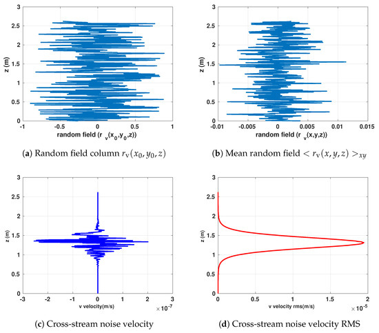
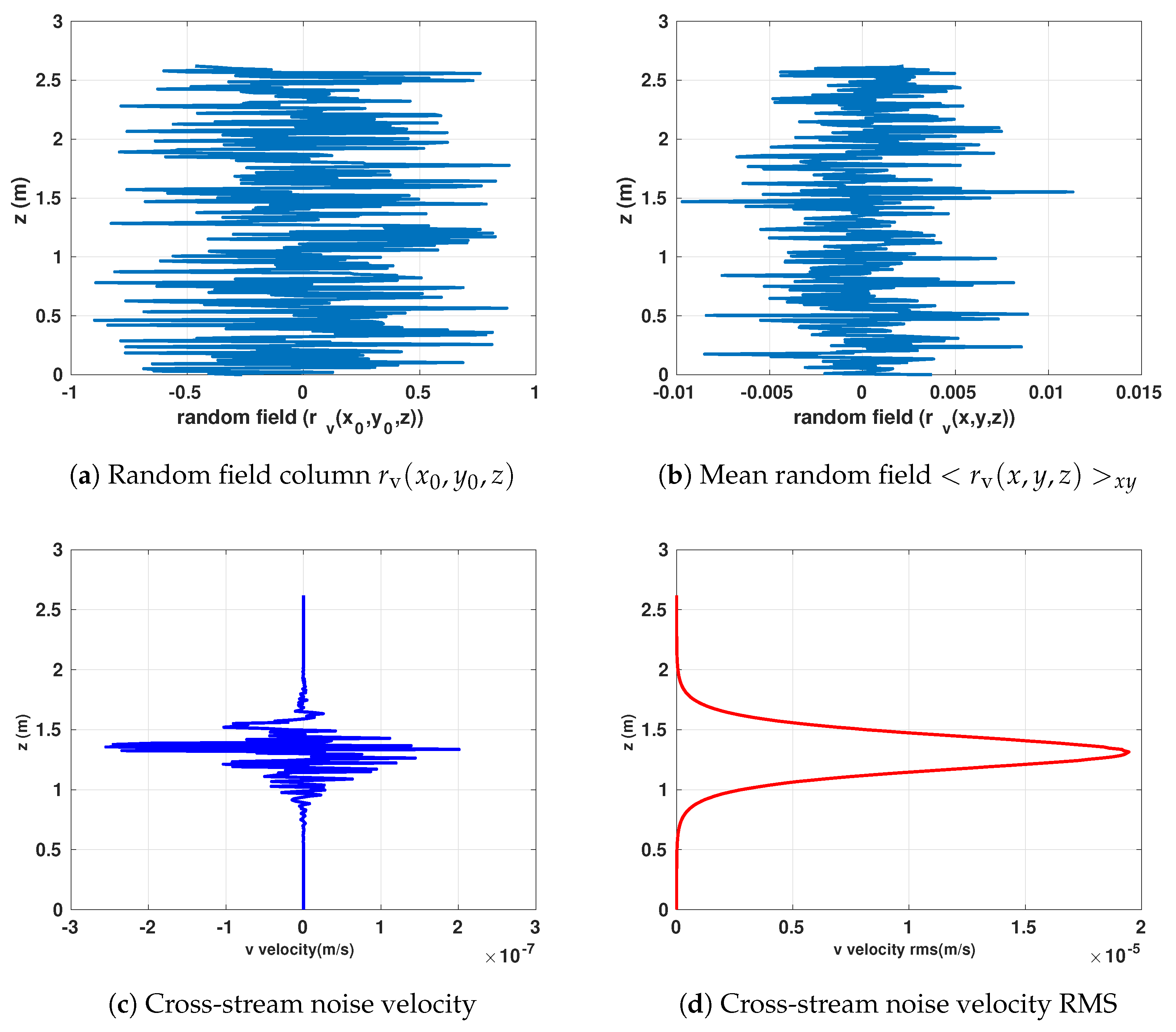
Figure 3. Various views of a random field $r_v(x,y,z)$ used in Equation (11), including (a) raw values from a representative vertical column, (b) horizontally averaged values as a function of z, (c) the resultant velocity noise profile using Equation (11), and (d) the root mean square (RMS) value of velocity noise calculated in the x-y plane.

Figure 3a shows a vertical column of $r_v(x_0,y_0,z)$ values from this random field. The random field, averaged in the x-y planes, is presented in Figure 3b. Figure 3c depicts the velocity noise $\tilde{v}$ (averaged in the x-y planes) associated with this random field, as calculated by Equation (11). Figure 3d presents the x-y root mean square (RMS) value of the velocity noise, which indicates that the velocity noise is focused on the shear layer.

2.1. Wavelength Calculation

The domain size $Lx,Ly,Lz,$ and $h_0$ must be chosen carefully for efficient memory usage and computation time. These choices are based on the linear stability analyses of the parallel flow [46,47]. Previous studies have determined an appropriate domain length based on a relationship of the following form:

$${\displaystyle \frac{L_x}{h_0}}={\displaystyle \frac{4\pi }{k_0{h}_0}}$$

(12)

where $k_0$ is the wavenumber. The slight dependence of $k_0$ on the Richardson number is ignored [46], and $k_0=0.90/h_0$ is chosen for all runs, following [39]. After replacing $k_0$, rearranging Equation (12), and using $h_0=0.38$ m (as used in the simulations discussed here), we obtain $L_x/h_0=13.96$, which is close to the work of [39], where they used $L_x/h_0=14$ to simulate a KH wave train.

We hypothesize that domain lengths ($L_x$) that are not an integer multiple of a natural KH billow wavelength $L_{\mathit{KH}}$ will result in a significant change to the turbulent energetics within the domain. The wavelength of instability in two-dimensional two-layer flow, as given by [15,23], is:

$$\lambda ={\displaystyle \frac{\pi \left(\mathsf{\Delta }{u}^2\right)}{g^{\prime }}}$$

(13)

where $\lambda$ represents the instability wavelength or the distance between billows, $\mathsf{\Delta }u$ is the velocity difference between the layers, and $g^{\prime }$ is the reduced gravity, where $g^{\prime }$ is ${\displaystyle \frac{g\mathsf{\Delta }\rho }{{\rho }_0}}$. Substituting the Richardson number $Ri={\displaystyle \frac{g^{\prime }{h}_0}{{\left(\mathsf{\Delta }u\right)}^2}}$ into Equation (13) yields

$$\lambda ={\displaystyle \frac{\pi h_0}{Ri}}$$

(14)

The Kelvin–Helmholtz wavelength $L_{\mathit{KH}}$ should vary with $\lambda$, but it may involve a constant $C_{\mathit{KH}}$ due to specific definitions of $h_0$ and $Ri$. So we define

$$L_{\mathit{KH}}={\displaystyle \frac{C_{KH}\pi h_0}{Ri}}$$

(15)

Initially, $C_{\mathit{KH}}$ is assumed to be equal to one, with the resulting length scale referred to as $L_{\mathit{KH}}^{*}$. The simulation results are then used to find an approximate value for $C_{\mathit{KH}}$, as discussed in Section 3.1.

2.2. Model Setup for Domain Length Analysis

The effects of domain length on the formation and dynamics of billows and the resulting turbulence are studied using a series of simulations wherein only the domain length $L_x$ is varied. Unlike the noise analysis simulations, no noise or perturbation is added to the velocity profiles. For all runs, the domain lengths of $L_y$ and $L_z$ remain constant at values of $L_y=0.64$ m and $L_z=2.62$ m, with $\mathsf{\Delta }y=\mathsf{\Delta }z=1$ cm, and $\mathsf{\Delta }x$ values can be obtained from Table 1. Initial velocity and density profiles are obtained from Equations (9) and (10), respectively. Table 1 reports the number of grid points and corresponding grid size for each case.

2.3. Model Setup for Noise Analysis

The noise analysis was conducted in two parts: In the first part, the random field $r_v(x,y,z)$ was kept constant, as in Equation (11), but the amplitude a of the noise was modified. In the second part, a remained constant but different realizations of the random field were used. In all simulations used for the noise analysis, $L_x$ was held constant at $Lx=5.24$ m.

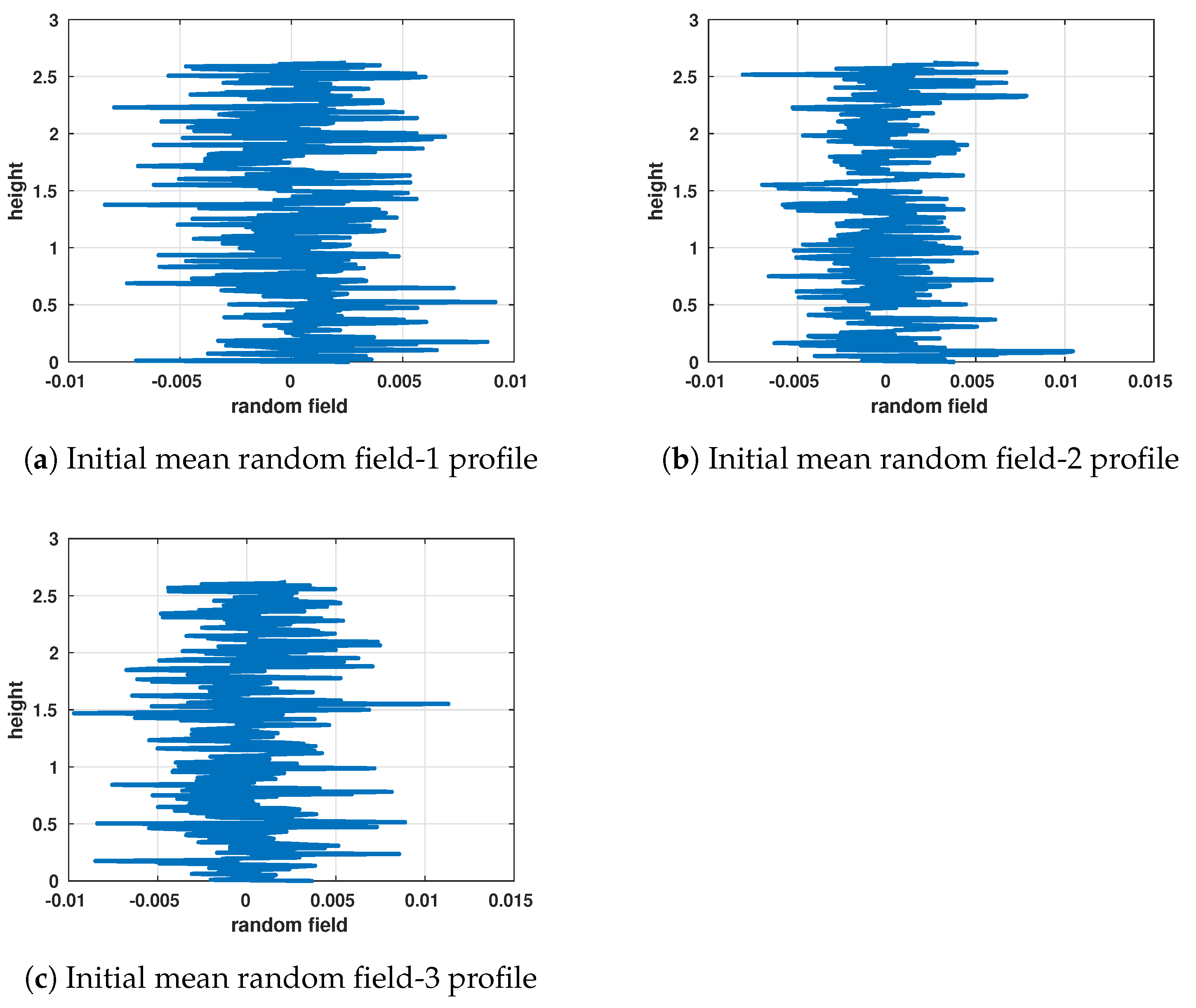
For the second part of the noise analysis, we used $a=0.01$ with three different realizations of the random field $r_v(x,y,z)$. Figure 4 shows these three different realizations averaged in the x-y plane. Seemingly minor differences between these fields may have a significant impact on the development of billows and the onset of turbulence.

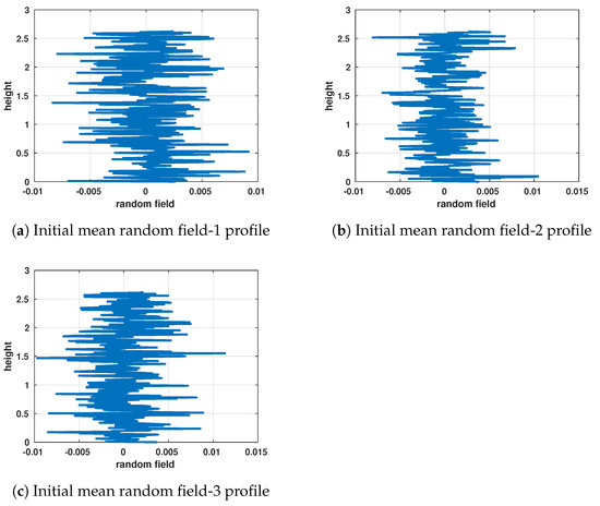
Figure 4. Horizontal mean values of three different realizations of the three-dimensional random field used in Equation (11).

3. Domain Length Analysis

The domain length analysis is based on evaluating the impact of varying $L_x$ on billow formation and duration, the number of billows generated, the billow wavelength, and mean turbulent quantities. For consistency, the grid resolution is kept constant in all directions. To facilitate comparison between the runs, time is non-dimensionalized by the buoyancy frequency N:

$$N=\sqrt[\hspace{0.25em}]{-{\displaystyle \frac{g}{{\rho }_0}}{\displaystyle \frac{\partial \rho }{\partial z}}}$$

(16)

Figure 5 presents simulation results at various domain lengths $L_x$, showing that as $L_x$ is increased, additional billows are generated. Note the increase from 1 to 4 billows as $L_x$ increases. Also, note that in cases such as in Figure 5e,f, where a single billow is split across the domain boundary, the billow is counted once.

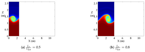
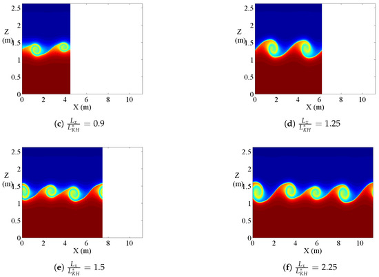
Figure 5. Simulation results at various domain lengths $L_x$ showing that additional billows are generated as $L_x$ is increased. Snapshots are extracted from each simulation during the period of well-defined billows.

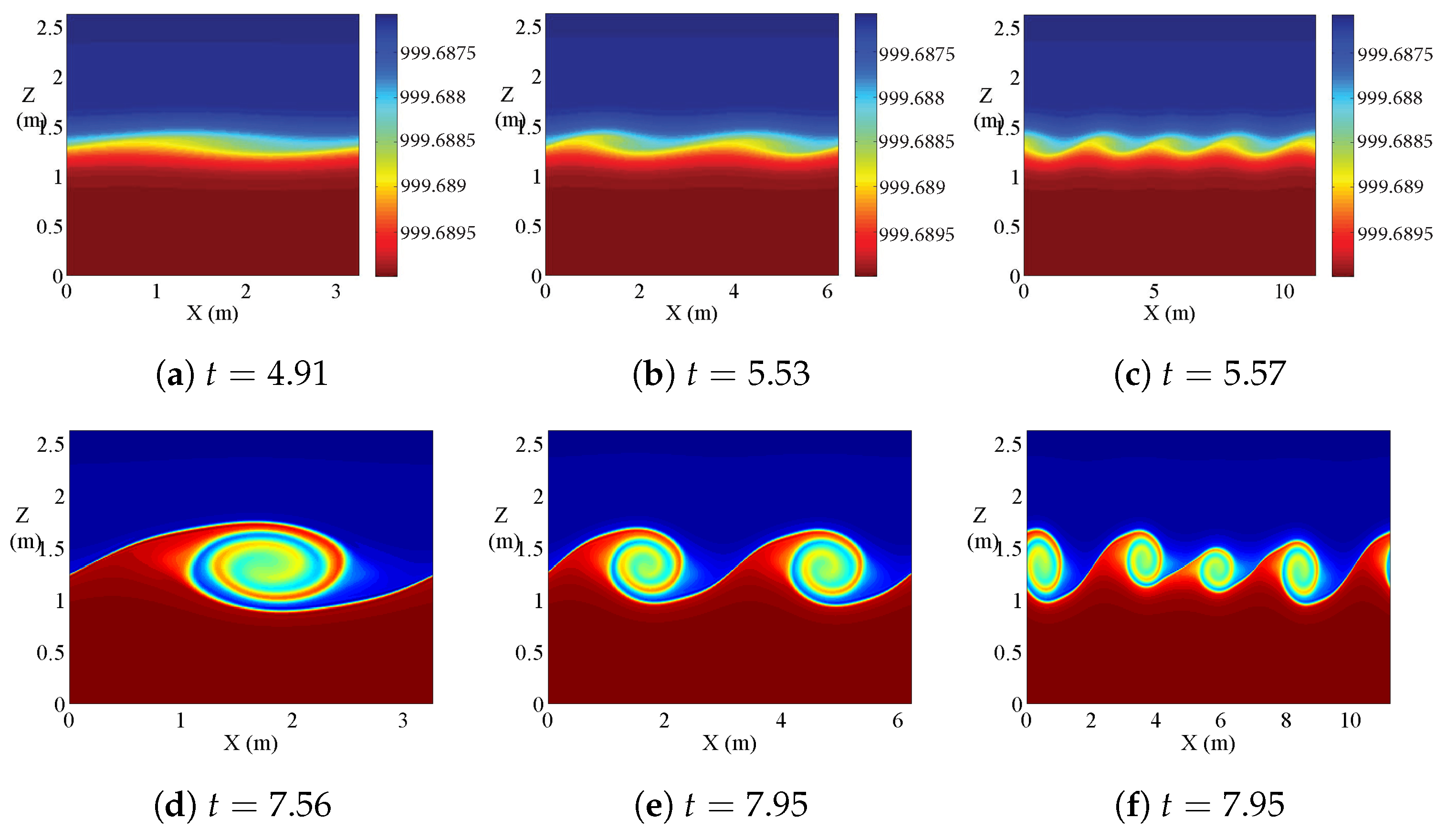
All simulations exhibit the same stages of evolution, as shown in Figure 6: In the first stage, the shear layer is not yet impacted by instabilities (not shown). After a few buoyancy periods, the billows start to form (Figure 6a–c), the number of which depends on the value of ${\displaystyle \frac{L_x}{L_{KH}^{*}}}$. The billows then roll up in a cat’s-eye formation, where the density gradients become more prominent, as shown in Figure 6d–f. After that, turbulence decays and the billows start to collapse and slowly lose strength. Following the decay of turbulence, the flow reaches a stable condition, which is shown by Figure 6m–o.

Figure 6. Density field for four billows corresponding to ${\displaystyle \frac{L_x}{L_{KH}^{*}}}$ of 0.65 (left column), 1.25 (middle), and 2.25 (right). Time is normalized by $1/N$ of Equation (16).

3.1. Determining C_KH

As shown in Figure 5, as the domain length is increased, the number of billows is also increased. We hypothesize that an increase in the number of billows must be tied to the natural billow wavelength $L_{\mathit{KH}}$ as the domain length $L_x$ is increased.

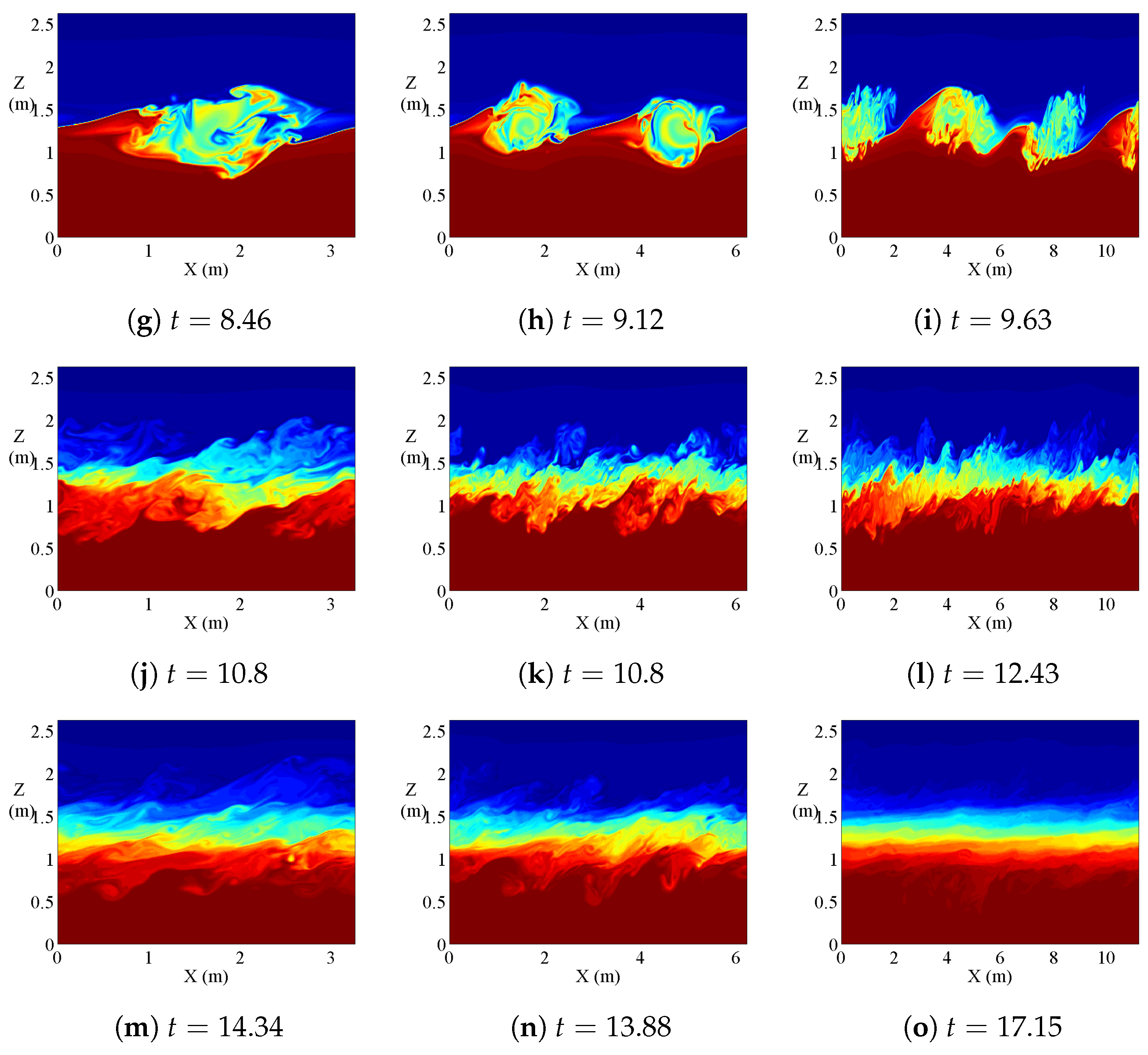
To consistently extract the billow wavelengths from the DNS results, the vertical gradient of the horizontal velocity (determined as the root mean square value of $\partial u/\partial z$, where u has been averaged in the cross stream, i.e., y, direction) is plotted against x, with peaks in $\partial u/\partial z$ corresponding to billow cores, as illustrated in Figure 7.

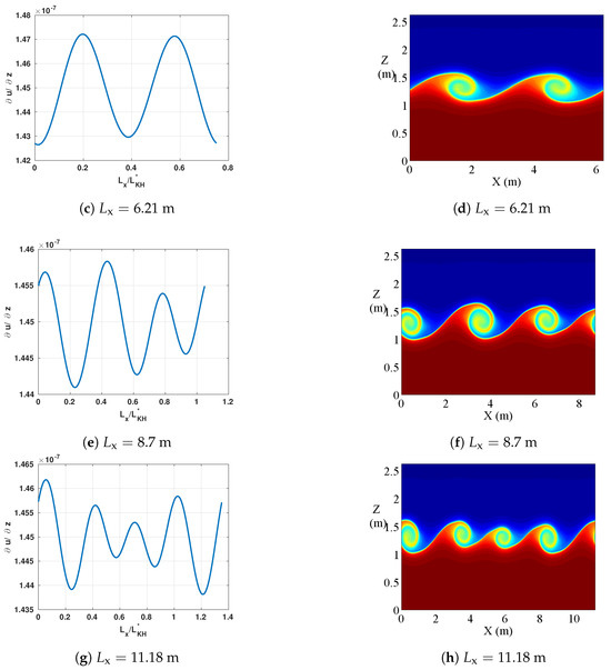
Figure 7. Identification of billow wave lengths. Left-column images present RMS values of ${\displaystyle \frac{\partial u}{\partial z}}$, where u has been averaged across the domain (i.e., the y-direction) as a function of x. Right-column snapshots provide a visual assessment of observed billows, as illustrated by fluid density.

Initialization of the billow phase is determined when distinct peaks are observed so that the billow wavelength $\lambda$ can be calculated. The end of the billow phase, as the billows decay to turbulence, is identified when there are many small peaks and it is impossible to distinguish the exact peak locations. This is identified in post-processing algorithms by a rapid variation in the wavelength values.

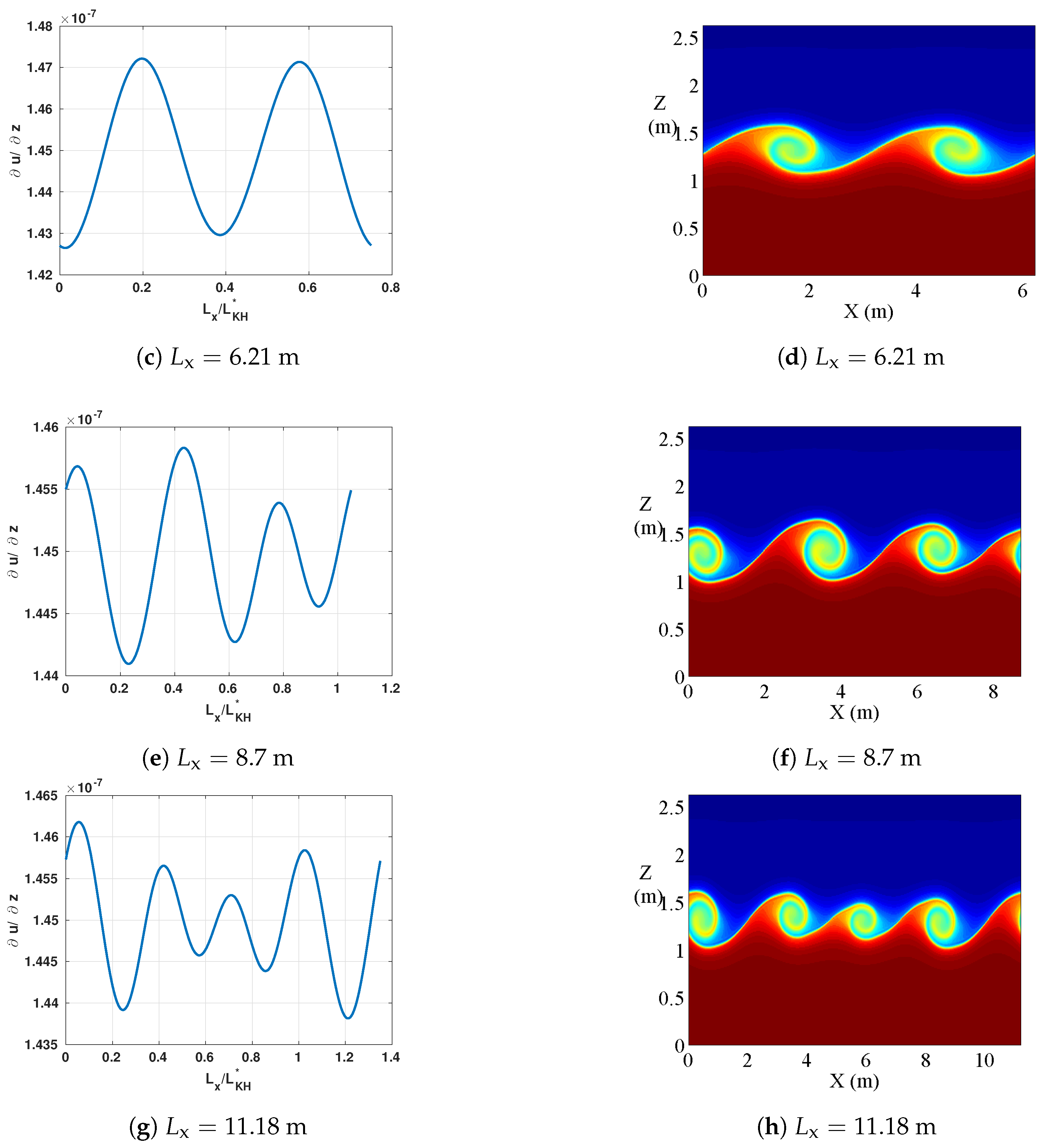
Note that the individual billow wavelength can evolve in time, although the sum of all billow wavelengths must always equal $L_x$. Profiles of billow wavelength as a function of time are shown for select simulations in Figure 8. The billow wavelengths in most of the simulations are reasonably consistent through the billow phase and are often punctuated by a rapid separation, which usually occurs around 6–8 buoyancy periods, when turbulence takes over.

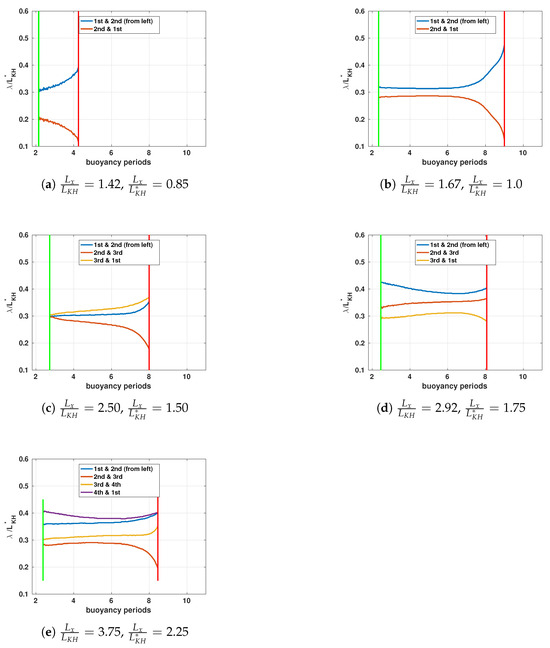
Figure 8. Normalized billow wavelengths for select simulations as a function of time, expressed as buoyancy periods. In each panel, the vertical lines represent the start and end of the “billow phase”.

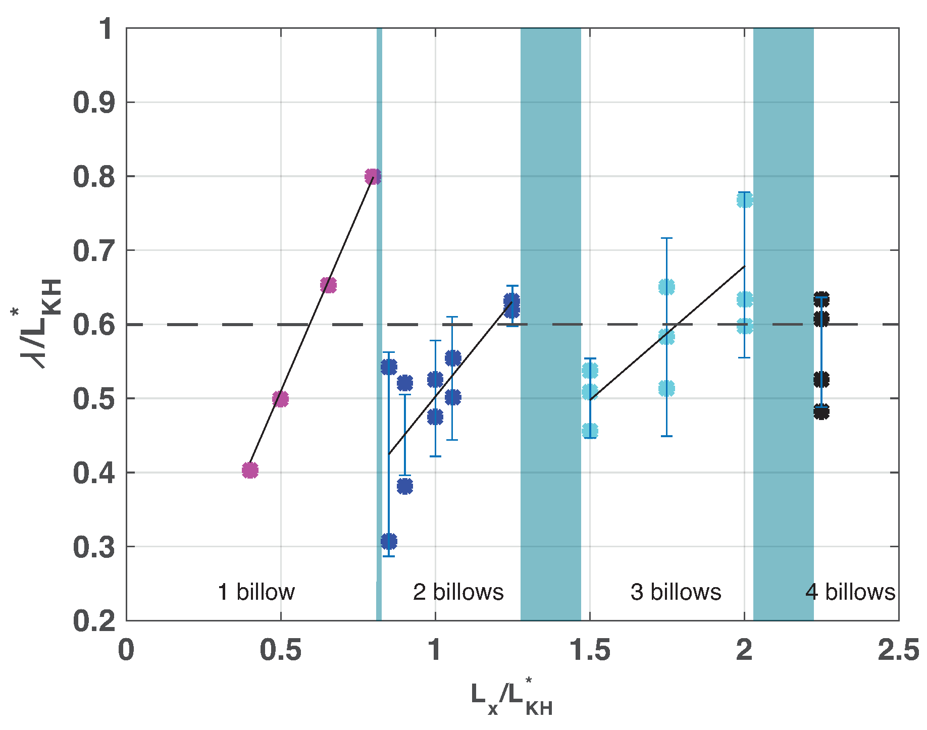
In Figure 9, the value of ${\displaystyle \frac{\lambda }{L_{KH}^{*}}}$ for each billow at the middle of each billow phase is plotted against the normalized domain length ${\displaystyle \frac{L_x}{L_{KH}^{*}}}$. For each simulation, the vertical bar represents the standard deviation of the observed wavelengths during the billow phase (in both time and space). The sloping line segments represent the mean ${\displaystyle \frac{\lambda }{L_{KH}^{*}}}$ values as defined by the domain length divided by the number of billows for each simulation. It is evident from Figure 9 that new billows are generated regularly with increasing domain length. The shaded columns represent domain length ranges where additional billows appear. In Figure 9, for the two-billow simulations, as the domain length increases, the wavelengths tend to converge. Similar behavior is less defined for the three-billow simulations.

Figure 9. Observed billow wavelengths normalized by $L_{KH}^{*}$ as a function of domain length normalized by $L_{KH}^{*}$ (i.e., assuming $C_{KH}=1$). The standard deviations of the observed wavelengths during the billow phase (in both time and space) are shown by the vertical bars. The sloping line segments represent the mean $\lambda /L_{KH}^{*}$. The shaded columns mark domain length ranges where additional billows appear. The points are colored based on the specified number of billows.

3.2. Billow Formation

If we assume that increasing the domain length by one KH billow wavelength (${\displaystyle \frac{\mathsf{\Delta }{L}_x}{L_{KH}}}=1$) will always result in the creation of one additional billow, we can use the numerical results to determine the value of $C_{KH}$. Graphically, this is shown in Figure 10, where the number of billows is plotted against the non-dimensional length ${\displaystyle \frac{L_x}{L_{KH}^{*}}}$. Here, the horizontal red bars indicate the uncertainty associated with transitions of increasing billow quantity. The slope of the line connecting these transition zones must be equal to ${(L_{KH}/L_{KH}^{*})}^{-1}$. Recognizing that $L_{KH}^{*}={\displaystyle \frac{L_{KH}}{C_{KH}}}$, it follows that the slope of this line is equal to ${\left(C_{KH}\right)}^{-1}$.

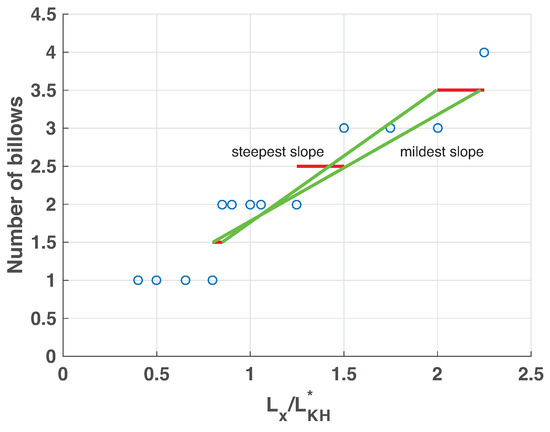
Figure 10. Number of billows vs. domain length normalized by $L_{KH}^{*}$. The green lines show the mildest and steepest slopes, and the horizontal red bars indicate the uncertainty associated with transitions of increasing billow quantities. The value of $C_{KH}$ can be determined as the slope of the line connecting transition regions, as shown.

In Figure 10, the mildest and steepest slopes (green lines) lead to $C_{KH}$ = 0.50 and 0.70, respectively. The average of these two values ($C_{KH}=0.6$) is shown by the dashed horizontal line (equivalent to $\lambda /L_{KH}=1$) in Figure 9. In all the following analyses, $L_{KH}$ rather than $L{*}_{KH}$ is used to normalize the domain length and the billow wavelength.

3.3. Billow Phase Duration

During the evolution of the billows and the resulting turbulence, there are several distinct phases, including the pre-billow, billow, and turbulent phases. Here, we use the model results to evaluate the duration of the billow phase as a function of the overall domain length.

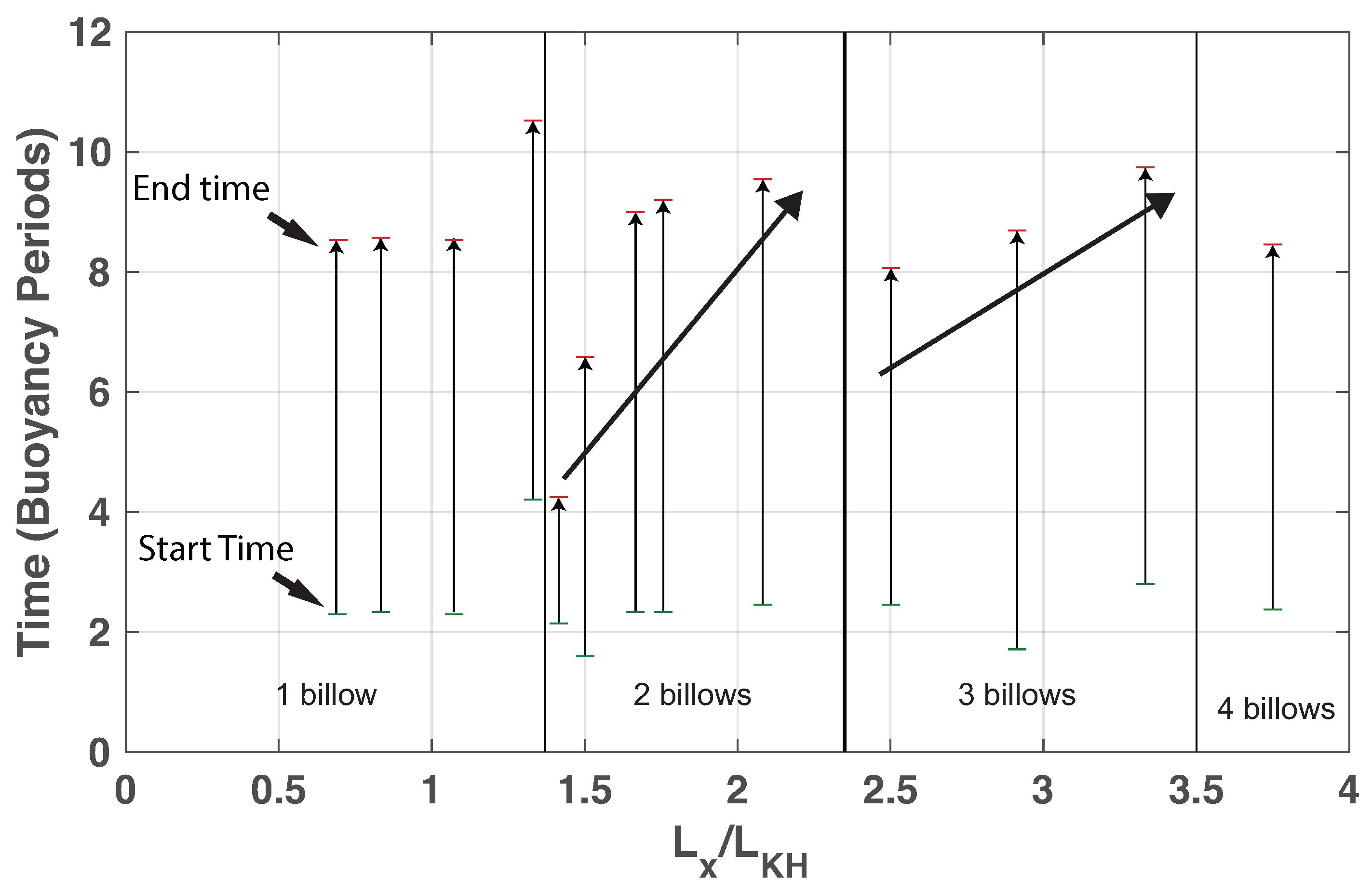
In Figure 11, the vertical arrows represent the start and end times and, thus, the duration of the billow phase for each simulation. For the one-billow simulations, all durations are approximately six buoyancy periods. In all simulations, the billow phase tends to start at approximately 2.17 buoyancy periods, but with increasing domain size, the duration of the billow phase increases, with the end time of the billow phase increasing from approximately four to nine buoyancy periods in the case of two billows. For the three-billow cases, similar but less-pronounced behavior is observed, with the billow phase generally starting around two buoyancy periods, while the end time gradually increases from 8 to 9.8 buoyancy periods. Only one four-billow simulation was run with a small $L_x/L_{KH}$, and it too follows a similar pattern, with a consistent start time and an end time that is reduced compared to the largest three-billow simulation. It is clear that a domain length that forces a shorter billow wavelength also results in a shorter-duration billow phase.

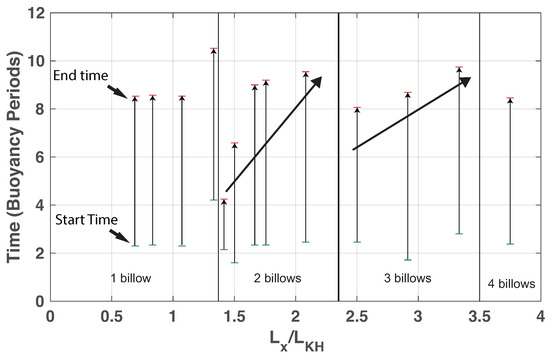
Figure 11. Duration of billow phase in terms of buoyancy periods from the start of the simulation, as identified by the tail and tip of each vertical arrow. Oblique arrows in the 2- and 3-billow ranges indicate the general trajectory of increased billow duration with increasing domain length.

3.4. Turbulent Quantities

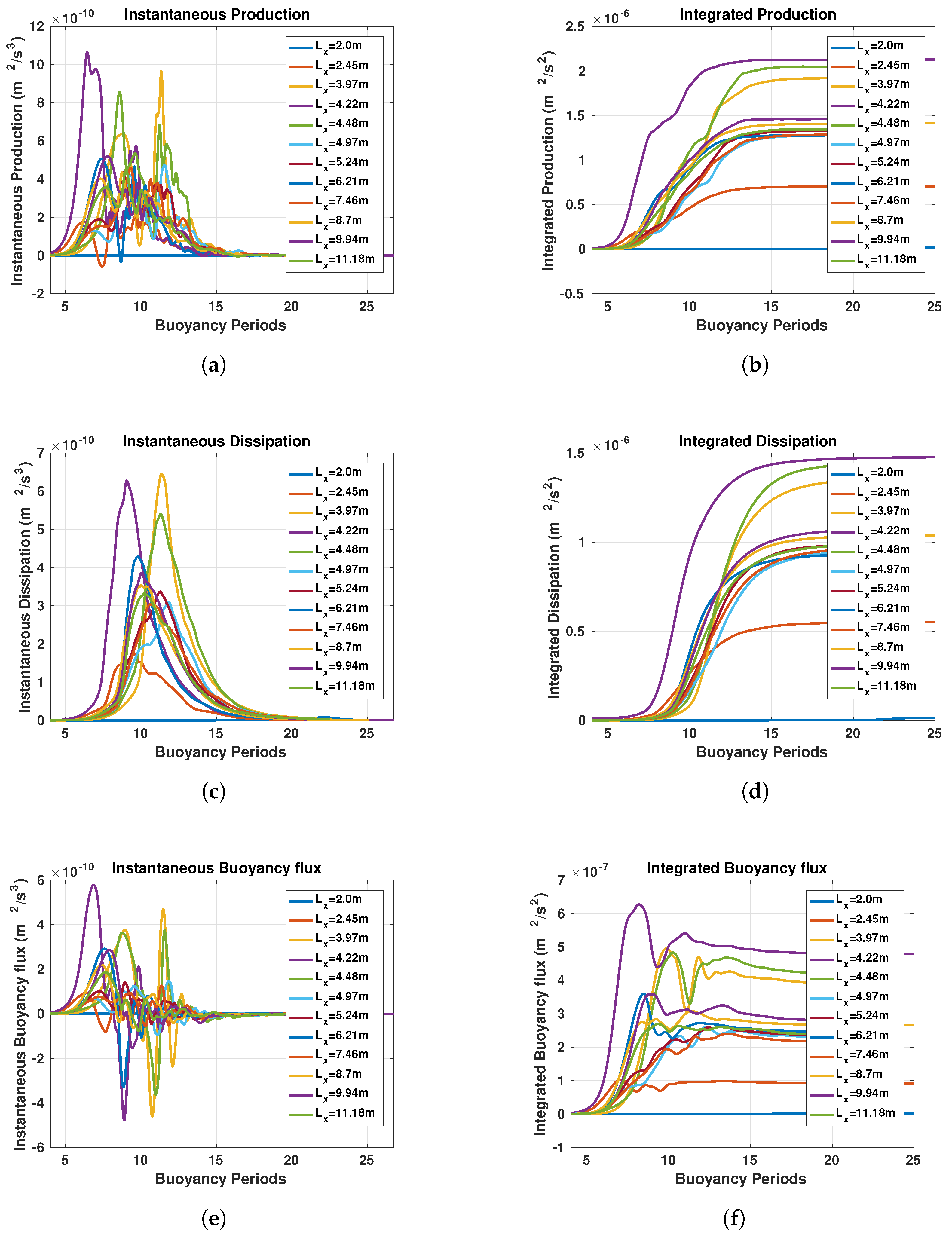
Figure 12 shows both instantaneous and integrated turbulent quantities for all 12 simulations with varying domain lengths, with turbulent data summarized in Table 2. In general, instantaneous values show similar behavior for all simulations, with the exception of the 2.0 m domain length ($L_x/L_{KH}=0.67$) simulation, for which turbulent quantities are several orders of magnitude lower than the other simulations. In all simulations, turbulence has essentially reached zero before approximately 20 buoyancy periods.

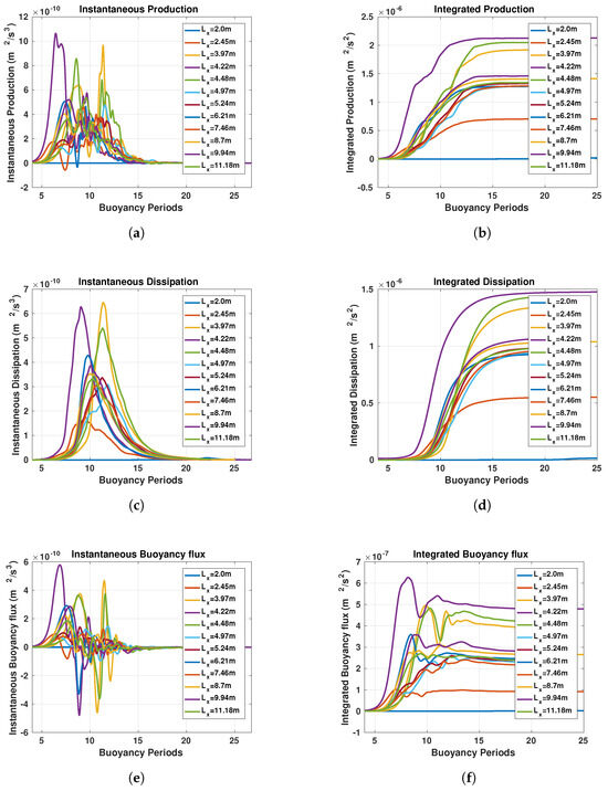
Figure 12. Time evolution of instantaneous (left column) and integrated (right column) turbulence quantities for different domain lengths.

Table 2. Effects of varying domain lengths $L_x$ on turbulence. Time is in buoyancy periods.

${\mathit{L}}_{\mathit{x}}/{\mathit{L}}_{\mathit{KH}}$	Flux Richardson Number	Mixing Efficiency	∫Production $\frac{{\mathit{m}}^2}{{\mathit{s}}^2}$	∫Buoyancy Flux $\frac{{\mathit{m}}^2}{{\mathit{s}}^2}$	∫Dissipation $\frac{{\mathit{m}}^2}{{\mathit{s}}^2}$	Start Time	End Time
0.67	0.13	0.1	1.94 × ${10}^{-8}$	2.03 × ${10}^{-9}$	1.56 × ${10}^{-8}$	2.34	8.61
0.84	0.16	0.13	7.05 × ${10}^{-7}$	9.22 × ${10}^{-8}$	5.50 × ${10}^{-7}$	2.34	8.58
1.09	0.28	0.2	1.95 × ${10}^{-6}$	3.93 × ${10}^{-7}$	1.38 × ${10}^{-6}$	2.34	8.61
1.33	0.28	0.2	1.92 × ${10}^{-6}$	3.86 × ${10}^{-7}$	1.36 × ${10}^{-6}$	4.21	10.52
1.42	0.32	0.22	2.13 × ${10}^{-6}$	4.79 × ${10}^{-7}$	1.48 × ${10}^{-6}$	2.14	4.25
1.50	0.29	0.2	2.05 × ${10}^{-6}$	4.21 × ${10}^{-7}$	1.44 × ${10}^{-6}$	1.60	6.59
1.67	0.24	0.17	1.28 × ${10}^{-6}$	2.29 × ${10}^{-7}$	9.42 × ${10}^{-7}$	2.34	9.00
1.76	0.23	0.17	1.33 × ${10}^{-6}$	2.36 × ${10}^{-7}$	9.87 × ${10}^{-7}$	2.34	9.20
2.08	0.26	0.19	1.28 × ${10}^{-6}$	2.46 × ${10}^{-7}$	9.28 × ${10}^{-7}$	2.46	9.55
2.50	0.22	0.16	1.29 × ${10}^{-6}$	2.15 × ${10}^{-7}$	9.62 × ${10}^{-7}$	2.46	8.07
2.92	0.25	0.18	1.41 × ${10}^{-6}$	2.65 × ${10}^{-7}$	1.04 × ${10}^{-6}$	1.29	8.69
3.33	0.26	0.19	1.46 × ${10}^{-6}$	2.80 × ${10}^{-7}$	1.07 × ${10}^{-6}$	2.81	9.74
3.75	0.23	0.17	1.35 × ${10}^{-6}$	2.34 × ${10}^{-7}$	9.94 × ${10}^{-7}$	2.38	8.46

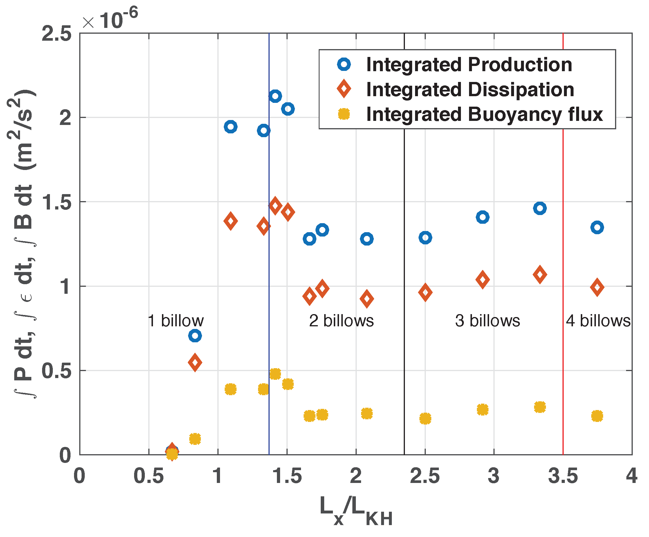
Integrated turbulent quantities tend to reach a constant value after 13 to 18 buoyancy periods, indicating that the turbulence phase is complete. The domain length has little impact on the time required to reach a stable condition. Integrated turbulent quantities, shown in Figure 12b,d,f, generally show good agreement among simulations for domain lengths greater than 5.2 m ($L_x/L_{KH}>1.5$). For domain lengths less than this threshold, considerable variability is observed. This can be seen more clearly in Figure 13, where the final integrated turbulent quantity values are plotted as a function of length $L_x/L_{KH}$. Here, it is clear that most of the observed variability occurs for the one-billow and early two-billow simulations, with variability spanning over two orders of magnitude. In general, the data suggest that wavelength compression (e.g., $L_x/L_{KH}$ values less than one for a one-billow simulation) results in less energetic turbulence overall, whereas wavelength stretching ($L_x/L_{KH}$ values greater than one for a one-billow simulation) tends to amplify turbulent energy. However, the two simulations at the low end of the two-billow regime stand in contrast to this observation. As domain lengths become larger, the degree of compression or stretching is minimized, and the effect becomes greatly reduced, although the trend is still visible, particularly in the three-billow regime. Mixing efficiency and flux Richardson number values are also tabulated in Table 2. Again, enhanced variability is seen for values of $L_x/L_{KH}<1.5$.

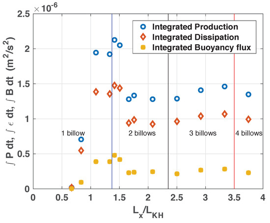
Figure 13. Net integrated turbulent quantities vs. normalized domain length $L_x/L_{KH}$. The blue, black, and red vertical lines mark the transitions from regimes with the specified number of billows formed in the simulations.

4. Noise Analysis

In this section, the impact of initialized noise is undertaken in two parts: first, noise amplitudes are varied with a constant random field (Section 4.1), and then, different random fields are used with a constant amplitude (Section 4.2).

4.1. Effect of Varying Noise

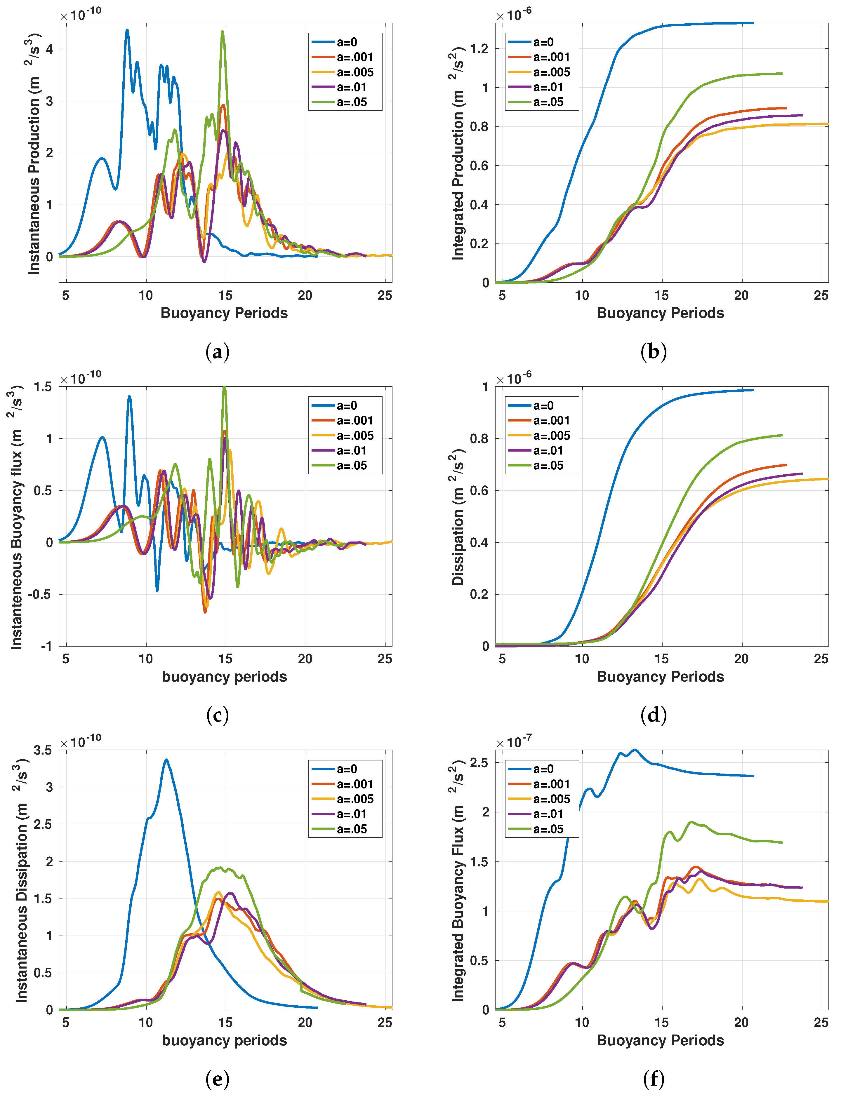
Consider the case with $Re=3610$, $Ri=0.12$, $Lx\left(m\right)=5.24$ m, $Ly\left(m\right)=2.62$ m, and $Lz\left(m\right)=0.64$ m. Here, one realization of the random field $r_v(x,y,z)$ (from Equation (11)) is frozen, and the amplitude a is varied from 0 to 0.05, as shown in Table 3. Initially, there is a quiescent period prior to billow formation. Here, the start of the turbulent event is identified as the point when the production rises to 0.001 of the overall maximum production value. The start and end times of each turbulent event are shown in Table 3, while Figure 14 shows the instantaneous values of turbulent quantities plotted against the buoyancy period; these values range from 0.1 to 1.5 buoyancy periods. This can also be seen in Figure 14, where the green line with 0.05 noise amplitude is the most delayed of all simulations.

Table 3. Effects of varying noise amplitude a on turbulence. Time is in buoyancy periods.

a	Flux Richardson Number	Mixing Efficiency	∫Production $\frac{{\mathit{m}}^2}{{\mathit{s}}^2}$	∫Buoyancy Flux $\frac{{\mathit{m}}^2}{{\mathit{s}}^2}$	∫Dissipation $\frac{{\mathit{m}}^2}{{\mathit{s}}^2}$	Start Time	End Time
0	0.17	0.239	1.33 × ${10}^{-6}$	2.36 × ${10}^{-7}$	9.87 × ${10}^{-7}$	4.52	21
0.001	0.14	0.177	8.94 × ${10}^{-7}$	1.24 × ${10}^{-7}$	6.98 × ${10}^{-7}$	5.65	22.8
0.005	0.14	0.173	8.15 × ${10}^{-7}$	1.10 × ${10}^{-7}$	6.44 × ${10}^{-7}$	5.61	22.7
0.01	0.14	0.187	8.58 × ${10}^{-7}$	1.24 × ${10}^{-7}$	6.65 × ${10}^{-7}$	5.72	22.6
0.05	0.16	0.207	4.78 × ${10}^{-7}$	5.86 × ${10}^{-8}$	3.71 × ${10}^{-7}$	6.04	22.5

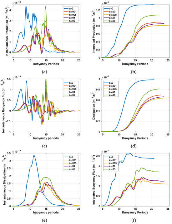
Figure 14. Time evolution of instantaneous (left column) and integrated (right column) turbulence quantities for different amplitudes of noise.

Figure 14c shows a change in buoyancy flux from negative to positive around time 13.5 to 15 for the case with noise velocities. This indicates a change in the buoyancy flux process from an energy sink to an energy source as unstable density profiles collapse. For a noiseless case, this event happens earlier at $t=12$. Similar behavior is found in Figure 14e, where dissipation reaches a peak around the same time. All the noise runs have some delay to reach the peak in dissipation as compared to the noiseless case. The overall process is delayed by about 1.5 to 2.3 buoyancy periods by the presence of noise.

Figure 14 shows the integrated values over time, as discussed in Section 1.1. Most field studies (e.g., [48,49]) yield only average turbulence values, so the integrated values, which can be used to determine an average value when divided by the event duration, may be the best way to compare DNS with field studies. Thus, the integrated values are used here to compare the effect of varying noise configurations.

In Figure 14b, it is clear that adding any noise reduces the overall TKE production values. The blue line, with zero noise, is 1.5 to 2 times higher than cases with noise. Changing the amplitude of the noise has a significant effect on both the flux Richardson number and the mixing efficiency: both are reduced compared to the zero-noise case. As shown in Table 3, the Ri_f values for noise cases are nearly constant at approximately 0.14 (compared to 0.17 for no-noise). The mixing efficiency is nearly constant, and the value is around 0.18 (compared to 0.239 for the zero-noise case). The largest amplitude $a=0.05$ increases both the flux Richardson number and the mixing efficiency compared to other noise cases.

4.2. Turbulence Quantities with Varying Random Field Realizations

For this section, different random fields $r_v(x,y,z)$ in Equation 11 are generated with a constant amplitude $(a=0.01)$. Table 4 shows the initial parameters for varying the random field cases and includes a no-noise run for comparison. Similar to Section 4.1, it is observed that any initial noise delays the onset of turbulence, as shown in Table 4.

Table 4. Turbulence quantities obtained with different random fields for $Re=3610$, $Ri=0.12$, $Lx=5.24$ m, $Ly=2.62$ m, and $Lz=0.64$ m.

Random Field	Noise Amplitude, a	Flux Richardson Number	Mixing Efficiency	∫Production $\frac{{\mathit{m}}^2}{{\mathit{s}}^2}$	∫Buoyancy Flux $\frac{{\mathit{m}}^2}{{\mathit{s}}^2}$	∫Dissipation $\frac{{\mathit{m}}^2}{{\mathit{s}}^2}$	Start Time
0	0	0.17	0.239	1.33 × ${10}^{-6}$	2.36 × ${10}^{-7}$	9.87 × ${10}^{-7}$	4.52
RF-1	0.01	0.19	0.261	1.40 × ${10}^{-6}$	2.67 × ${10}^{-7}$	1.02 × ${10}^{-6}$	5.57
RF-2	0.01	0.14	0.185	8.58 × ${10}^{-7}$	1.24 × ${10}^{-7}$	6.65 × ${10}^{-7}$	5.73
RF-3	0.01	0.12	0.158	4.91 × ${10}^{-7}$	5.46 × ${10}^{-8}$	4.00 × ${10}^{-7}$	6.04

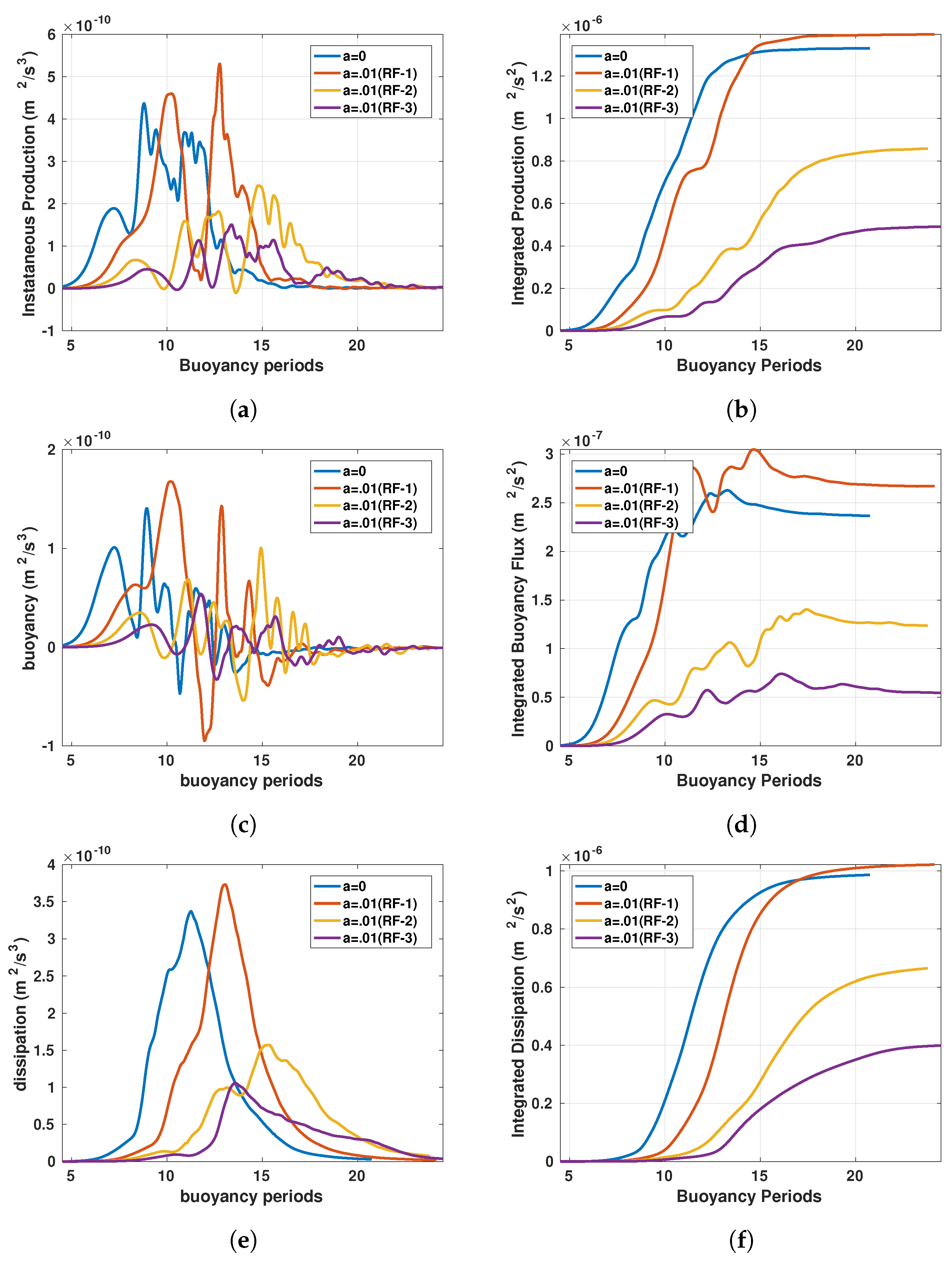
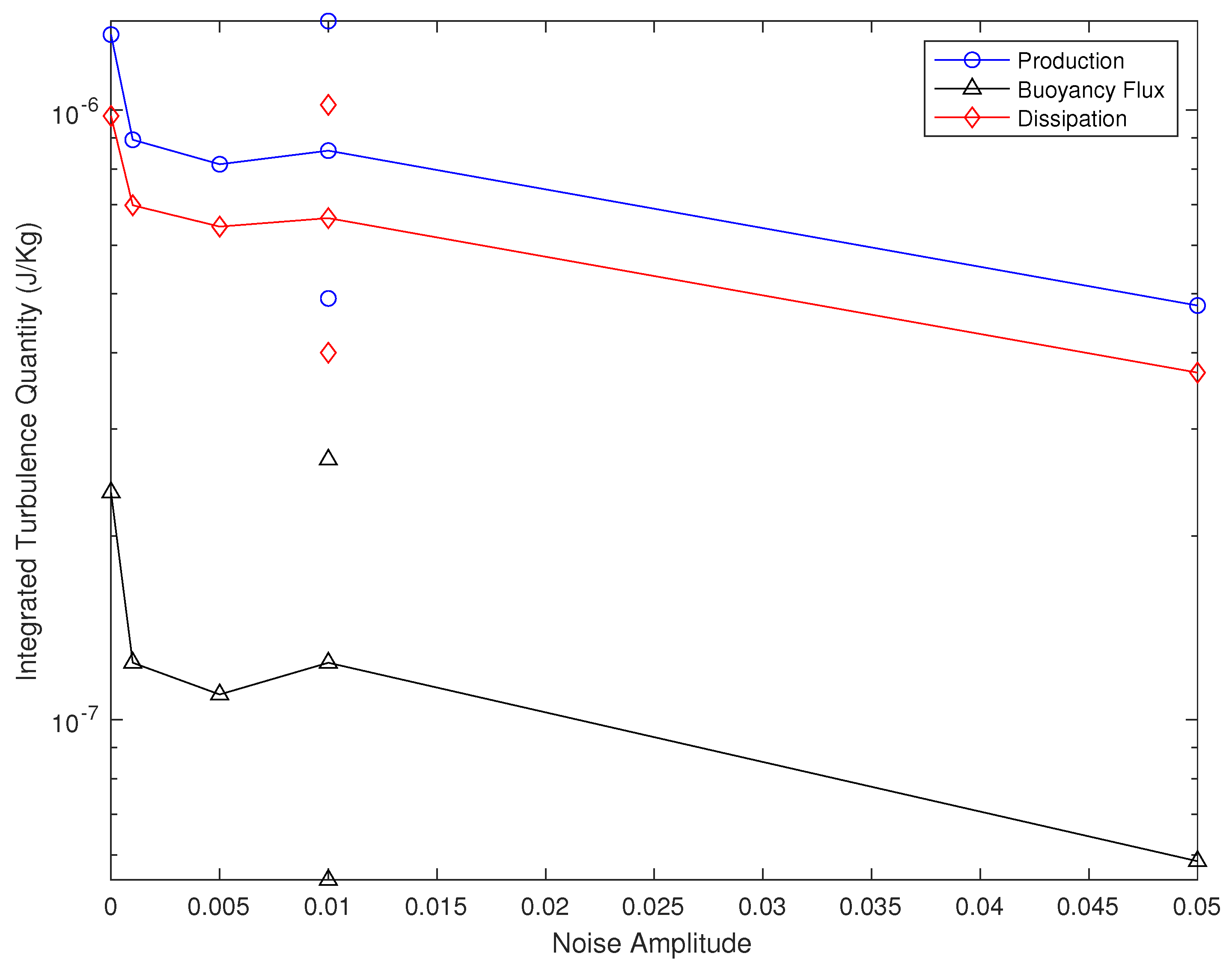
Figure 15 shows the instantaneous and integrated values of turbulent quantities. Note that all three versions of the random field have an onset of turbulence that is delayed compared to the no-noise case, which is surprising and counterintuitive given that noise is often added to DNS runs to seed the generation of instabilities. The magnitude of turbulent quantities for RF-1 is comparable to and slightly higher than the no-noise case, but the other two random-noise cases show a marked decrease (up to a factor of ∼3) in the magnitude of the turbulent quantities. Figure 16 compares the magnitude of variability in the integrated turbulent quantities as a function of both noise amplitude and random field realization. Here, symbols connected by the solid lines represent the same random field with different noise amplitudes, as discussed in the previous section, and the floating symbols at a noise amplitude of 0.01 represent different random fields. While noise amplitudes greater than zero but less than 0.01 result in relatively constant integrated turbulent quantities, there is a marked decay in turbulent energy at the larger (0.05) noise amplitude. Interestingly, the realization of the random field appears to have an impact of similar or greater magnitude compared to the noise amplitudes tested.

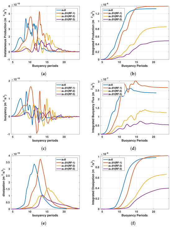
Figure 15. Time evolution of instantaneous (left column) and integrated (right column) turbulence quantities for different random fields but constant noise amplitude.

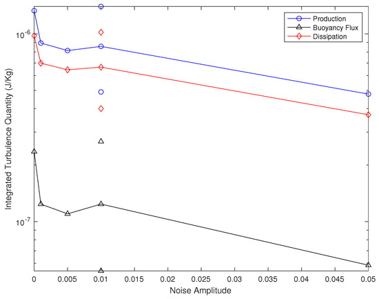
Figure 16. Integrated turbulence quantities vs. noise amplitude and random field realizations. Symbols aligned with a noise amplitude of 0.01 represent alternative random fields.

The exact mechanism for this phenomenon is not clear. Although it appears that noise typically has a damping effect on turbulence, occasionally, amplification of turbulence is observed. We hypothesize that the nature and magnitude of the ultimate impact of applied noise on the resulting turbulence field is due to the exact location of noise elements within the shear layer. More specifically, the location of noise elements relative to one another may have significant impacts on instability formation, and the phenomenon is non-linear and difficult to predict. Some random arrangements of noise elements may have a damping effect, while other arrangements may have an amplifying effect. It should also be noted that both the flux Richardson number and mixing efficiency values in Table 4 vary significantly for the various realizations of the noise field, further suggesting that the location of specific noise elements in the domain may lead to significantly different turbulent outcomes.

Similarly, we further suspect that increasing the amplitude of the noise will only serve to amplify the effect of the specific arrangement of noise elements. If a specific realization of noise elements has a damping effect, then increasing the noise amplitude will enhance that effect, and this will be similar for realizations that are likely to enhance turbulence.

Our results are generally consistent with those of Kaminski and Smyth [38], Dong et al. [50], and Brucker and Sarkar [51], who observed a damping effect on turbulence related to higher-amplitude perturbations, which ultimately led to lower mixing efficiencies. However, the case of random noise investigated here may be dynamically distinct from a perturbation of a given wave form, where the growth of the KH perturbation may be directly affected by the periodicity of the perturbation.

5. Conclusions and Summary

In this work, Kelvin–Helmholtz billows were studied using DNS at a Reynolds number of 3610 and a Richardson number of 0.12. In the first part of this study, the domain size in the streamwise direction was varied from 0.2 m to 11.18 m, which produced between one and four billows in the domain. In the second part, the effect of initial noise on the generated turbulence was explored: first by comparing runs with the same random field but different noise amplitudes and then by using a constant noise amplitude with different realizations of the random field.

The following conclusions can be made from the results presented in this work, which also capture the novelty and contributions of the study:

• Noise should be used with caution in DNS runs because it can significantly alter the timing and magnitude of resulting turbulence in a manner that is difficult to predict.
• Adding any noise delays turbulence, thereby increasing the computational time by up to 30–40 percent.
• The noise amplitude has a minimum impact on overall turbulence quantities. The nature of the random field is much more important.
• Using different realizations of the field has a significant impact on the timing and magnitude of turbulence.
• Turbulent quantities associated with different random fields can vary by a factor of up to three to five.
• The natural Kelvin–Helmholtz billow wavelength is found to be consistent with $L_{KH}={\displaystyle \frac{C_{KH}\pi h_0}{Ri}}$, with $C_{KH}=0.6$ determined from the numerical runs.
• Net production, dissipation, and buoyancy flux are approximately constant with the domain length as long as $Lx>1.5L_{KH}$.
• Domain lengths that force a shorter billow wavelength also result in a shorter-duration billow phase.
• An additional billow forms, on average, for every increase in domain length by $L_{KH}$.

Future work will include a sensitivity analysis using statistical methods to better understand the variability introduced by different noise realizations and will quantify the impact on turbulent quantities.

References

- Helmholtz, P. XLIII. on discontinuous movements of fluids. Lond. Edinb. Dublin Philos. Mag. J. Sci. 1868, 36, 337–346. [Google Scholar] [CrossRef]
- Kelvin, L.O.R.D. Hydrokinetic solutions and observations. Phil. Mag. 1871, 10, 155–168. [Google Scholar]
- Caulfield, C.-C.P. Open questions in turbulent stratified mixing: Do we even know what we do not know? Phys. Rev. Fluids 2020, 5, 110518. [Google Scholar] [CrossRef]
- De Silva, I.; Fernando, H.; Eaton, F.; Hebert, D. Evolution of Kelvin–Helmholtz billows in nature and laboratory. Earth Planet. Sci. Lett. 1996, 143, 217–231. [Google Scholar] [CrossRef]
- Blaauwgeers, R.; Eltsov, V.B.; Eska, G.; Finne, A.P.; Haley, R.P.; Krusius, M.; Ruohio, J.J.; Skrbek, L.; Volovik, G.E. Shear flow and Kelvin–Helmholtz instability in superfluids. Phys. Rev. Lett. 2002, 89, 155301. [Google Scholar] [CrossRef] [PubMed]
- Hebert, D.; Moum, J.; Paulson, C.; Caldwell, D. Turbulence and internal waves at the equator. Part II: Details of a single event. J. Phys. Oceanogr. 1992, 22, 1346–1356. [Google Scholar] [CrossRef]
- Moum, J.N.; Hebert, D.; Paulson, C.A.; Caldwell, D.R. Turbulence and internal waves at the equator. Part I: Statistics from towed thermistors and a microstructure profiler. J. Phys. Oceanogr. 1992, 22, 1330–1345. [Google Scholar] [CrossRef]
- Dalin, P.; Pertsev, N.; Frandsen, S.; Hansen, O.; Andersen, H.; Dubietis, A.; Balciunas, R. A case study of the evolution of a Kelvin–Helmholtz wave and turbulence in noctilucent clouds. J. Atmos.-Sol.-Terr. Phys. 2010, 72, 1129–1138. [Google Scholar] [CrossRef]
- Bau, H.H. Kelvin–Helmholtz instability for parallel flow in porous media: A linear theory. Phys. Fluids 1982, 25, 1719–1722. [Google Scholar] [CrossRef]
- Ong, R.S.B.; Roderick, N. On the Kelvin–Helmholtz instability of the earth’s magnetopause. Phys. Fluids 1982, 25, 1–10. [Google Scholar] [CrossRef]
- Smyth, W.D. Smyth, Secondary Kelvin–Helmholtz instability in weakly stratified shear flow. J. Fluid Mech. 2003, 497, 67–98. [Google Scholar] [CrossRef]
- Mashayek, A.; Peltier, W. The zoo of secondary instabilities precursory to stratified shear flow transition. Part 1 shear aligned convection, pairing, and braid instabilities. J. Fluid Mech. 2012, 708, 5–44. [Google Scholar] [CrossRef]
- Caulfield, C. Layering, Instabilities, and Mixing in Turbulent Stratified Flows. Annu. Rev. Fluid Mech. 2021, 53, 113–145. [Google Scholar] [CrossRef]
- Van Haren, H.; Gostiaux, L. A deep ocean Kelvin–Helmholtz billow train. Geophys. Res. Lett. 2010, 37, L03605. [Google Scholar] [CrossRef]
- MacDonald, D.G.; Carlson, J.; Goodman, L. On the heterogeneity of stratified-shear turbulence: Observations from a near-field river plume. J. Geophys. Res. Oceans 2013, 118, 6223–6237. [Google Scholar] [CrossRef]
- Maslowe, S. The generation of clear air turbulence by nonlinear waves. Stud. Appl. Math. 1972, 51, 1–16. [Google Scholar] [CrossRef]
- Kelly, R.; Maslowe, S. The nonlinear critical layer in a slightly stratified shear flow. Stud. Appl. Math. 1970, 49, 301–326. [Google Scholar] [CrossRef]
- Drazin, P. Kelvin–Helmholtz instability of finite amplitude. J. Fluid Mech. 1970, 42, 321–335. [Google Scholar] [CrossRef]
- Klaassen, G.P.; Peltier, W.R. Evolution of finite amplitude Kelvin–Helmholtz billows in two spatial dimensions. J. Atmos. Sci. 1985, 42, 1321–1339. [Google Scholar] [CrossRef]
- Patnaik, P.C.; Sherman, F.S.; Corcos, G.M. A numerical simulation of Kelvin–Helmholtz waves of finite amplitude. J. Fluid Mech. 1976, 73, 215–240. [Google Scholar] [CrossRef]
- Miles, J.W.; Howard, L.N. Note on a heterogeneous shear flow. J. Fluid Mech. 1964, 20, 331–336. [Google Scholar] [CrossRef]
- Drazin, P.; Howard, L. Hydrodynamic stability of parallel flow of inviscid fluid. Adv. Appl. Mech. 1966, 9, 1–89. [Google Scholar]
- Turner, J.S. Buoyancy Effects in Fluids; Cambridge University Press: Cambridge, UK, 1973. [Google Scholar]
- Tennekes, H.; Lumley, J.L. Lumley, A First Course in Turbulence; MIT Press: Cambridge, MA, USA, 1972. [Google Scholar]
- Kundu, P.K.; Cohen, I.M.; Dowling, D.R. Fluid Mechanics; Academic Press: Cambridge, MA, USA; Elsevier Inc.: Amsterdam, The Netherlands, 2016. [Google Scholar]
- Gayen, B.; Sarkar, S. Negative turbulent production during flow reversal in a stratified oscillating boundary layer on a sloping bottom. Phys. Fluids 2011, 23, 101703. [Google Scholar] [CrossRef]
- Burchard, H.; Bolding, K. Comparative analysis of four second-moment turbulence closure models for the oceanic mixed layer. J. Phys. Oceanogr. 2001, 31, 1943–1968. [Google Scholar] [CrossRef]
- Staquet, C. Two-dimensional secondary instabilities in a strongly stratified shear layer. J. Fluid Mech. 1995, 296, 73–126. [Google Scholar] [CrossRef]
- Salehipour, H.; Caulfield, C.P.; Peltier, W.R. Turbulent mixing due to the holmboe wave instability at high Reynolds number. J. Fluid Mech. 2016, 803, 591–621. [Google Scholar] [CrossRef]
- Liu, C.-L.; Kaminski, A.K.; Smyth, W.D. Turbulence and mixing from neighbouring stratified shear layers. J. Fluid Mech. 2024, 987, A8. [Google Scholar] [CrossRef]
- Liu, C.-L.; Kaminski, A.K.; Smyth, W.D. The effects of boundary proximity on Kelvin–Helmholtz instability and turbulence. J. Fluid Mech. 2023, 966, A2. [Google Scholar] [CrossRef]
- Liu, C.-L.; Kaminski, A.K.; Smyth, W.D. The butterfly effect and the transition to turbulence in a stratified shear layer. J. Fluid Mech. 2022, 953, A43. [Google Scholar] [CrossRef]
- Yang, A.J.K.; Timmermans, M.-L.; Lawrence, G.A. Asymmetric Kelvin-Helmholtz instabilities in stratified shear flows. Phys. Rev. Fluids 2024, 9, 14501. [Google Scholar] [CrossRef]
- Yang, A.J.K.; Tedford, E.W.; Olsthoorn, J.; Lawrence, G.A. Sensitivity of wave merging and mixing to initial perturbations in Holmboe instabilities. Phys. Fluids 2022, 34, 126610. [Google Scholar] [CrossRef]
- VanDine, A.; Pham, H.T.; Sarkar, S. Turbulent shear layers in a uniformly stratified background: DNS at high Reynolds number. J. Fluid Mech. 2021, 916, A42. [Google Scholar] [CrossRef]
- Smyth, W.D.; Moum, J.N. Anisotropy of turbulence in stably stratified mixing layers. Phys. Fluids 2000, 12, 1343–1362. [Google Scholar] [CrossRef]
- Rahmani, M. Kelvin–Helmholtz Instabilities in Sheared Density Stratified Flows. Ph.D. Thesis, University of British Columbia, Vancouver, BC, Canada, 2011. [Google Scholar]
- Kaminski, A.K.; Smyth, W.D. Stratified shear instability in a field of pre-existing turbulence. J. Fluid Mech. 2019, 862, 639–658. [Google Scholar] [CrossRef]
- Smyth, W.D.; Moum, J.N. Length scales of turbulence in stably stratified mixing layers. Phys. Fluids 2000, 12, 1327–1342. [Google Scholar] [CrossRef]
- Caulfield, C.; Peltier, W. The anatomy of the mixing transition in homogeneous and stratified free shear layers. J. Fluid Mech. 2000, 413, 1–47. [Google Scholar] [CrossRef]
- Desjardins, O.; Blanquart, G.; Balarac, G.; Pitsch, H. High order conservative finite difference scheme for variable density low Mach number turbulent flows. J. Comput. Phys. 2008, 227, 7125–7159. [Google Scholar] [CrossRef]
- Pierce, C.D.; Moin, P. Progress-variable approach for large-eddy simulation of non-premixed turbulent combustion. J. Fluid Mech. 2004, 504, 73–97. [Google Scholar] [CrossRef]
- Kim, J.; Moin, P. Application of a fractional-step method to incompressible Navier-Stokes equations. J. Comput. Phys. 1985, 59, 308–323. [Google Scholar] [CrossRef]
- Van der Vorst, H.A. Iterative Krylov Methods for Large Linear Systems; Cambridge University Press: Cambridge, UK, 2003. [Google Scholar]
- Courant, R.; Friedrichs, K.; Lewy, H. Über die Partiellen differenzengleichungen der mathematischen physik. Math. Ann. 1928, 100, 32–74. [Google Scholar] [CrossRef]
- Hazel, P. Numerical studies of the stability of inviscid stratified shear flows. J. Fluid Mech. 1972, 51, 39–61. [Google Scholar] [CrossRef]
- Smyth, W.; Peltier, W. The transition between Kelvin–Helmholtz and Holmboe instability: An investigation of the overreflection hypothesis. J. Atmos. Sci. 1989, 46, 3698–3720. [Google Scholar] [CrossRef]
- MacDonald, D.G.; Chen, F. Role of mixing in the structure and evolution of a buoyant discharge plume. J. Geophys. Res. Oceans 2006, 111, C11002. [Google Scholar]
- Barringer, M.; Price, J. Mixing and spreading of the mediterranean overflow. J. Phys. Oceanogr. 1997, 27, 1654–1677. [Google Scholar] [CrossRef]
- Dong, W.; Tedford, E.W.; Rahmani, M.; Lawrence, G.A. Lawrence, Sensitivity of vortex pairing and mixing to initial perturbations in stratified shear flows. Phys. Rev. Fluids 2019, 4, 063902. [Google Scholar] [CrossRef]
- Brucker, K.A.; Sarkar, S. A comparative study of self-propelled and towed wakes in a stratified fluid. J. Fluid Mech. 2010, 652, 373–404. [Google Scholar] [CrossRef]
Disclaimer/Publisher’s Note: The statements, opinions and data contained in all publications are solely those of the individual author(s) and contributor(s) and not of MDPI and/or the editor(s). MDPI and/or the editor(s) disclaim responsibility for any injury to people or property resulting from any ideas, methods, instructions or products referred to in the content. |
© 2024 by the authors. Licensee MDPI, Basel, Switzerland. This article is an open access article distributed under the terms and conditions of the Creative Commons Attribution (CC BY) license (https://creativecommons.org/licenses/by/4.0/).