Analysis of Temperature Field in the Dielectrophoresis-Based Microfluidic Cell Separation Device

Abstract

Cell separation techniques based on dielectrophoresis are of high interest as an effective method of performing cell separation non-invasively on cells. However, dielectrophoresis devices have the problem that cells in the device are exposed to a high-temperature environment due to the generation of Joule heat caused by high-voltage application and dielectric-loss heat when the applied voltage is AC voltage. There is concern that the heat generated in the device may affect cell viability, cell cycle and apoptosis induction. In this study, the temperature field inside the dielectrophoretic cell separation device was experimentally and numerically investigated. The temperature rise at the bottom of the flow channel in the device was measured using the LIF method, and the thermofluidal behavior of the device was numerically simulated by adopting a heat generation model that takes the Joule and dielectric-loss heating into account in the energy equation. The temperature rise in the device was evaluated and the effect of the heat generation on cells in the device is discussed.

1. Introduction

In recent years, techniques for the rapid and accurate separation of rare cells from a large number of diverse cell populations have attracted much attention. In particular, cell separation techniques based on dielectrophoresis have attracted considerable interest because they are non-invasive to cells [1,2,3]. Dielectrophoresis is a phenomenon in which an electromechanical force (dielectrophoretic force) is generated on dielectric particles placed in a non-uniform electric field [4]. Non-uniform electric fields induce translational motion of a biological cell along the electric field gradient. The electric field gradient necessary for the occurrence of cells’ movement can be generated by integrating microelectrodes on a substrate within a microfluidic channel. Dielectrophoresis cell separation devices require relatively high applied voltages to generate electric field gradients to manipulate cells. The application of this principle is expected to lead to the development of important technologies, such as separation, concentration, purification, and manipulation of cells in the fields of regenerative medicine and clinical medicine [5,6,7]. On the other hand, challenges exist for cell separation devices based on dielectrophoresis technology. That is, the cells in the device are exposed to a high-temperature environment due to the generation of Joule heat originating from the strong electric field in the solution and, when the electric field is AC, the generation of dielectric-loss heat in the solution and the device itself. The degree of heating mostly depends on the solution conductivity, applied voltage, and device dimension. A large power density is locally generated in the small area near to the edge of the microelectrode even when the applied voltage is not so strong. This could give rise to a large temperature increase in the solution in the vicinity of the edges of electrode. Thus, there is concern that the heat generated in cell separation devices may affect cell viability, cell cycle and apoptosis induction [8].

The heat generation $Q$ in cell separation devices using dielectrophoresis is mainly Joule heat due to the conductivity of the solution, plus dielectric-loss heat of the dielectric materials in a high-frequency AC electric field [4,9]. Therefore, $Q$ is denoted as

$$Q=\left(\sigma +2\pi f{ϵ}_w\tan \delta \right)E^2$$

(1)

where $\sigma$ is the conductivity of the solution, $f$ is the frequency of the AC electric field, ${ϵ}_w$ is the electric permittivity of the solution, $\tan \delta$ is the dielectric-loss tangent and $E$ is the electric field. Usually, Joule heating is more pronounced in high-conductivity solutions ($\sigma$ > $~$100 mS/m), such as cell-culture media and phosphate buffer ($\sigma ~$1 S/m). Therefore, the dielectric-loss heating is much smaller than the Joule heating, and can be ignored when these high-conductivity electrolyte solutions were used for cell separation. It has been reported that biological cells can survive for 6 h at a temperature $~$42 °C [10] and even 150 s at 48 °C [11].

Many previous studies have focused on Joule heating in high-conductivity solutions, especially, numerically predicting the temperature rise due to Joule heating in a microdevice. Tay et al. numerically predicted the temperature rise of around 10 °C when the AC voltage of 100 V_pp was applied to the solution with the conductivity of $\sigma$ = 47 mS/m in the microdevice [12], Sridharan et al. numerically predicted the temperature rise of around 30 °C when the DC voltage of 100 V was applied to the solution with the conductivity of $\sigma$ = 100 mS/m [13]. Kale et al. numerically predicted the temperature rise of around 12 °C when the AC voltage of 350 V_pp was applied to the solution with the conductivity of $\sigma$ = 100 mS/m in the microdevice [14]. Nakano et al. conducted experiments using the laser-induced fluorescence (LIF) method and numerical simulations. Their results demonstrated that the temperature rise was 30 °C when an AC voltage of 3 kV_pp was applied to the solution with the conductivity of $\sigma$ = 10 mS/m [15]. On the other hand, Kwak et al. focused on the frequency dependence of the heat generation, and measured the temperature rise in the microchannel due to the dielectric-loss heating. The results were compared with numerical simulations [16].

An effective way to reduce excessive temperature rise is to use a low-conductivity solution, such as mannitol solution. Mannitol solution is a non-electrolyte and isotonic solution that is somewhat detrimental to cell viability due to its composition. However, it has the advantage of significantly reducing the heat generation. Recently, the authors developed a microfluidic cell separation device adopting the AC dielectrophoresis, and achieved a cell separation ratio of over 90% for live and dead human-mammary cells suspended in a low-conductivity ($\sigma$ = 1 mS/m) mannitol solution [17]. In this study, the temperature field analysis in the developed device under the condition of the cell separation operation was conducted to evaluate the temperature rise that has baneful influence on cell viability. The temperature rise at the bottom surface of the device where the interdigitated electrodes were placed was measured using the LIF method. The thermofluidal behavior of the device was investigated using numerical simulation. A heat generation model considering Joule heat and dielectric-loss heat was adopted in the governing equations of the energy transport. Temperature rise in the device was evaluated, and the effect of the temperature rise on cells in the device was discussed.

2. Materials and Methods

The temperature rise over the surface of the bottom face of the micro flow channel was measured using the LIF method. Fluorescence images of the bottom face of the micro flow channel were captured with a confocal laser-scanning microscope and the transient of the distributions of temperature rise over the surface of the bottom face of the micro flow channel was obtained by image analysis. The methods of the preparation of the fluorescent dye, image acquisition, and interpretation of the fluorescence image to temperature distributions are presented.

2.1. Sample Preparation

Rhodamine B, which is widely used in the LIF method, was used as the fluorescent dye [18,19]. A 300 mM mannitol solution, widely used for cell separation, was used as the solvent for the sample solution [17,20,21] and the solution conductivity was prepared to $\mathsf{\sigma }=1\times {10}^{-3}$ S/m using cell culture medium, and the final concentration of Rhodamine B (Sigma 83695-250MG; ex 553 nm, em 627 nm) was set at 20 µM [22,23].

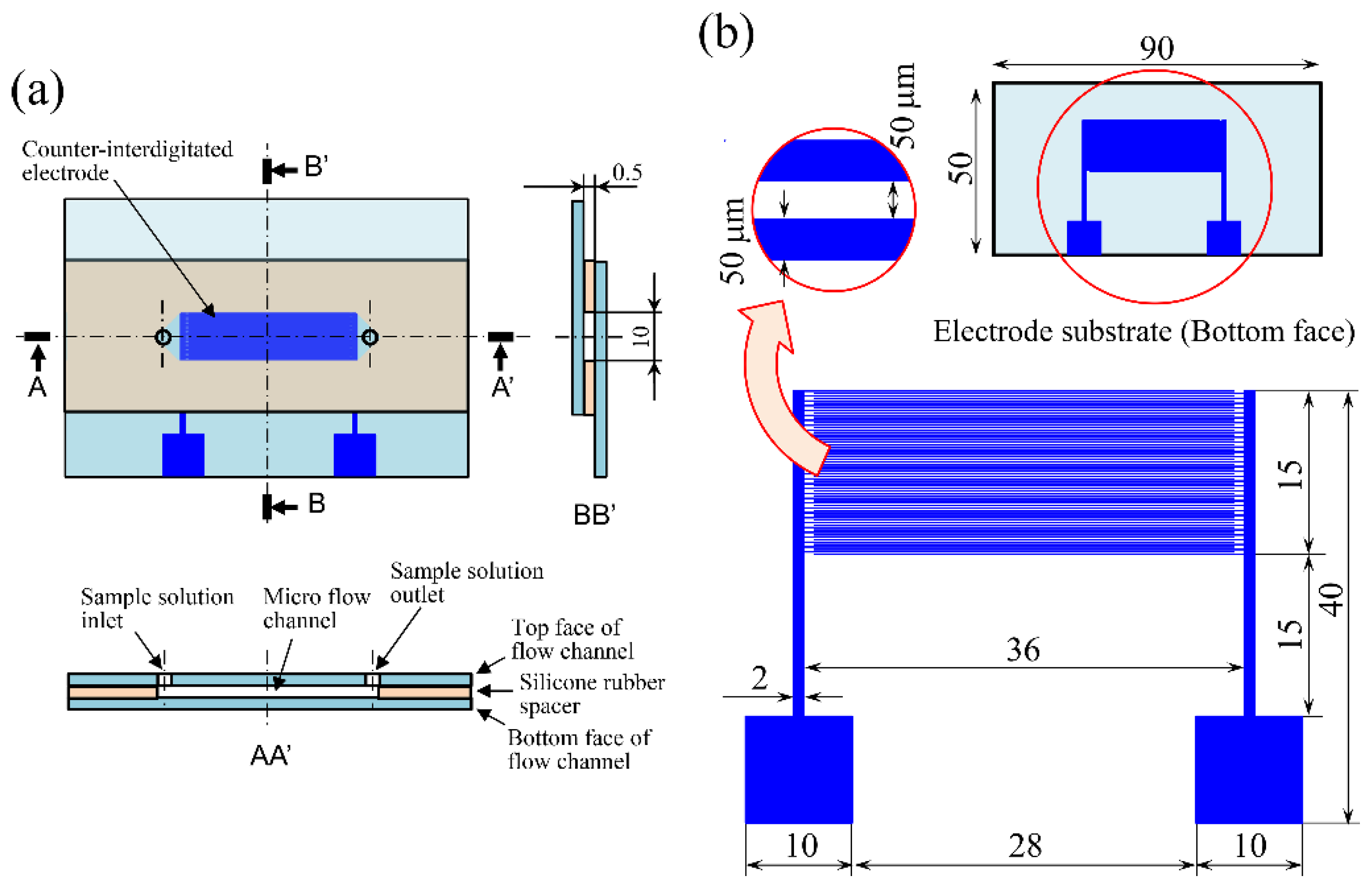
2.2. Device Fabrication

Figure 1 shows schematics of (a) the proposed cell separation device and (b) the counter-interdigitated electrode substrate. The device has a parallel-plate microfluidic-channel structure consisting of a planar indium-tin-oxide (ITO) transparent electrode on the top and an electrode substrate on the bottom, with the channel height maintained at 0.5 mm by a silicone rubber spacer. The width and length of the microfluidic channel are 10 mm and 36 mm, respectively. The counter-interdigitated electrode consists of 75 pairs of thin strip-shaped electrodes of 36 mm length aligned in parallel along the flow direction of the microfluidic channel. For the electrode width and spacing, 3$~$4 times the cell diameter ($~$16 mm) [24] was thought to be desirable for the effective separation of cells [24,25]. Therefore, the electrode width and spacing were taken as 50 mm [17]. The electrode substrates were fabricated by vacuum deposition of a 300 nm-thick aluminum film onto a glass planar plate of the size 50 $\times$ 90 mm using standard photolithography.

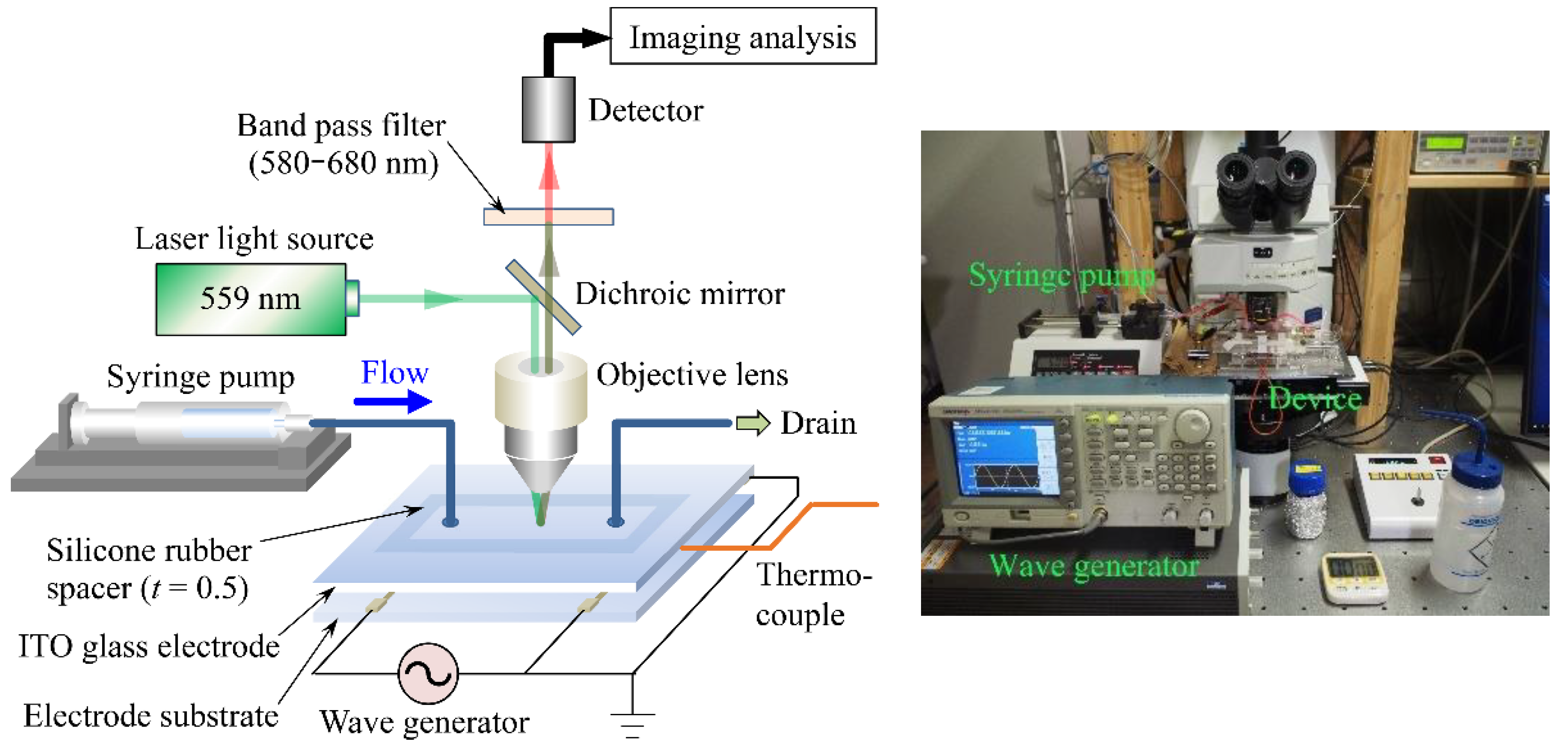
2.3. Experimental Setup

A schematic diagram of the primary part of the experimental setup is shown in Figure 2. The experimental setup mainly consisted of the cell separation device, a syringe pump (YSP-201, YMC, Shimogyoku, Kyoto, Japan) and a wave generator (AFG3151, Tektronix, Beaverton, OR, USA). The device was set on the stage of the confocal laser-scanning microscope (FV-1000, Olympus, Shinjyuku, Tokyo, Japan) and the microscope focus was set on the surface of the counter-interdigitated electrode where heat generation was expected to be most pronounced. The top electrode plate and one of the paired counter-interdigitated electrodes were connected to the ground side of the wave generator, and the remaining one of the electrodes to the high-voltage side of the wave generator using lead wires. The syringe set on the syringe pump was connected to the sample solution introduction port at the microfluidic upstream end via a silicone tube. After the syringe was filled with 5 mL of sample solution and the sample solution flowed into the microfluidic channel at a constant flow rate, using the syringe pump to degas the microfluidic channel, the wave generator was switched on and an AC voltage of 20 V_pp was applied to the device [17]. Fluorescence images were acquired using a laser beam with an excitation wavelength of 559 nm and a bandpass filter with a wavelength range of 570–670 nm. To ensure that the acquired images were free from white-out and black-out, the intensity of the laser light was adjusted by checking the histogram of the fluorescence image brightness to ensure that the fluorescence intensity was within the dynamic range of the detector. Before the electric-field application, the initial temperature of the sample solution was measured and a reference image was acquired at the initial temperature with no voltage application (0 V_pp). The temperature of the sample solution was measured using a T-type thermocouple. After acquiring the reference image, the voltage was applied to the device and we began acquiring fluorescence images at the same time. Time-lapse images of the fluorescence image were acquired every 30 s from the start of the voltage application ($t$ = 0) until $t$ = 300 s elapsed. The acquired fluorescence images were stored in an uncompressed TIFF format with a resolution of 1024 $\times$ 1024 pixels. The experiments were performed by varying the frequency f to $f$ = 20, 200 and 2000 kHz and the sample solution flow rate $Q$ to $Q$ = 5, 10 and 20 mL/h. For the values of $f$ and $Q$, the same values as those used in the cell separation experiments [17] were used.

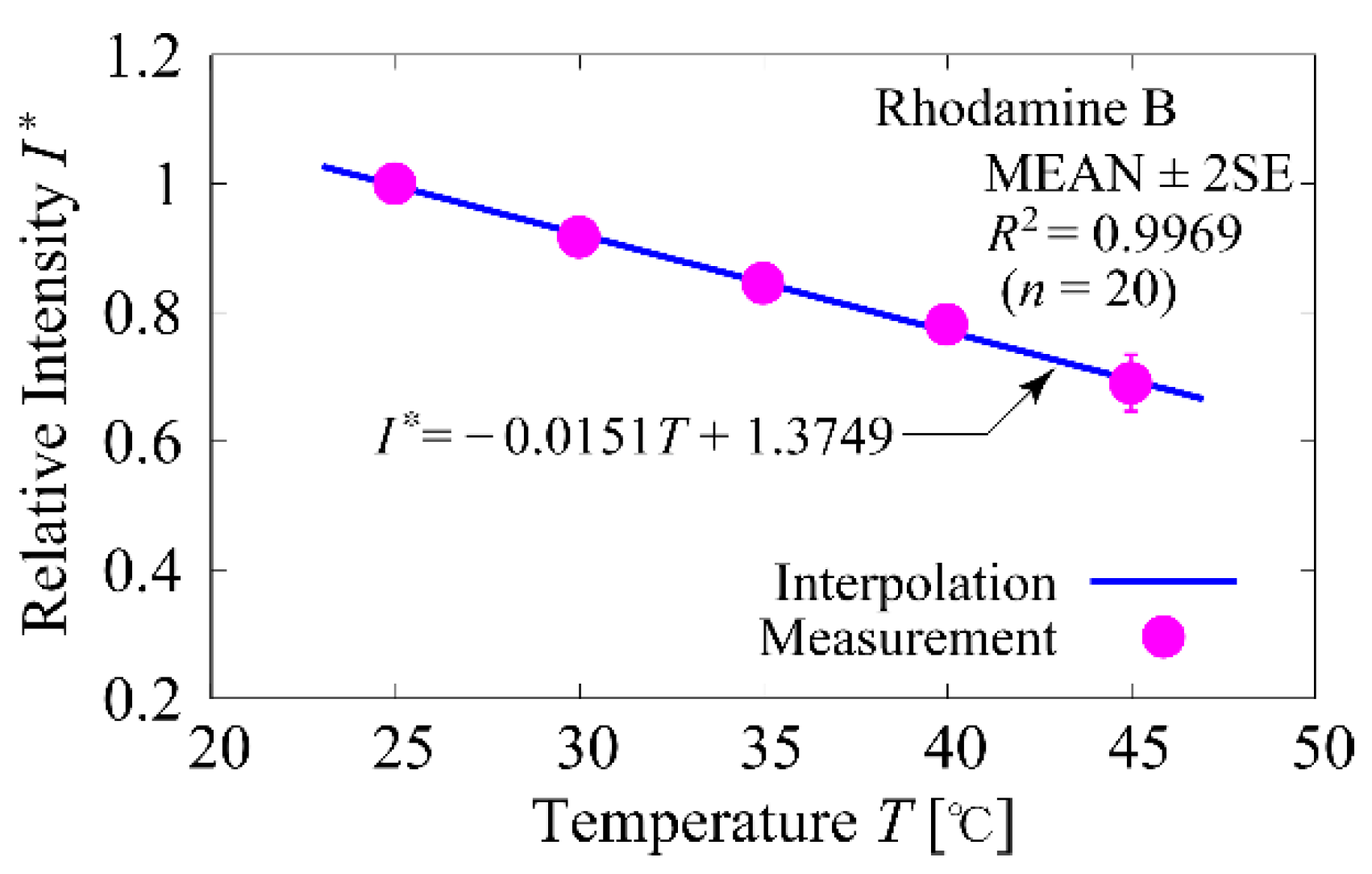
2.4. Temperature Calibration

Calibration of the temperature against the fluorescence intensity ratio was performed using a plate reader (DTX-880, Beckman Coulter, Brea, CA, USA). 60 µL of the sample solution was dispensed into 10 wells of the microtiter plate and another 60 µL of 300 mM mannitol solution with solution conductivity $\sigma$ = 1 mS/m was dispensed into another 10 wells for background acquisition. The wavelength of the excitation light was set to 535 nm and the wavelength of the bandpass filter to 625 nm, and the temperature in the chamber of the plate reader was changed every 5 °C from 25 °C to 45 °C to acquire fluorescence intensity. For calibration, the background fluorescence intensity was subtracted from the fluorescence intensity of the sample solution acquired at each temperature. The calibration curve obtained is shown in Figure 3. The number of measurements was n = 20 and the plots represent MEAN ± 2SE. Fluorescence intensities were normalized to that at a temperature of 25 °C. The straight line was linearly interpolated by the least-squares method and the coefficient of determination was R² = 0.9969.

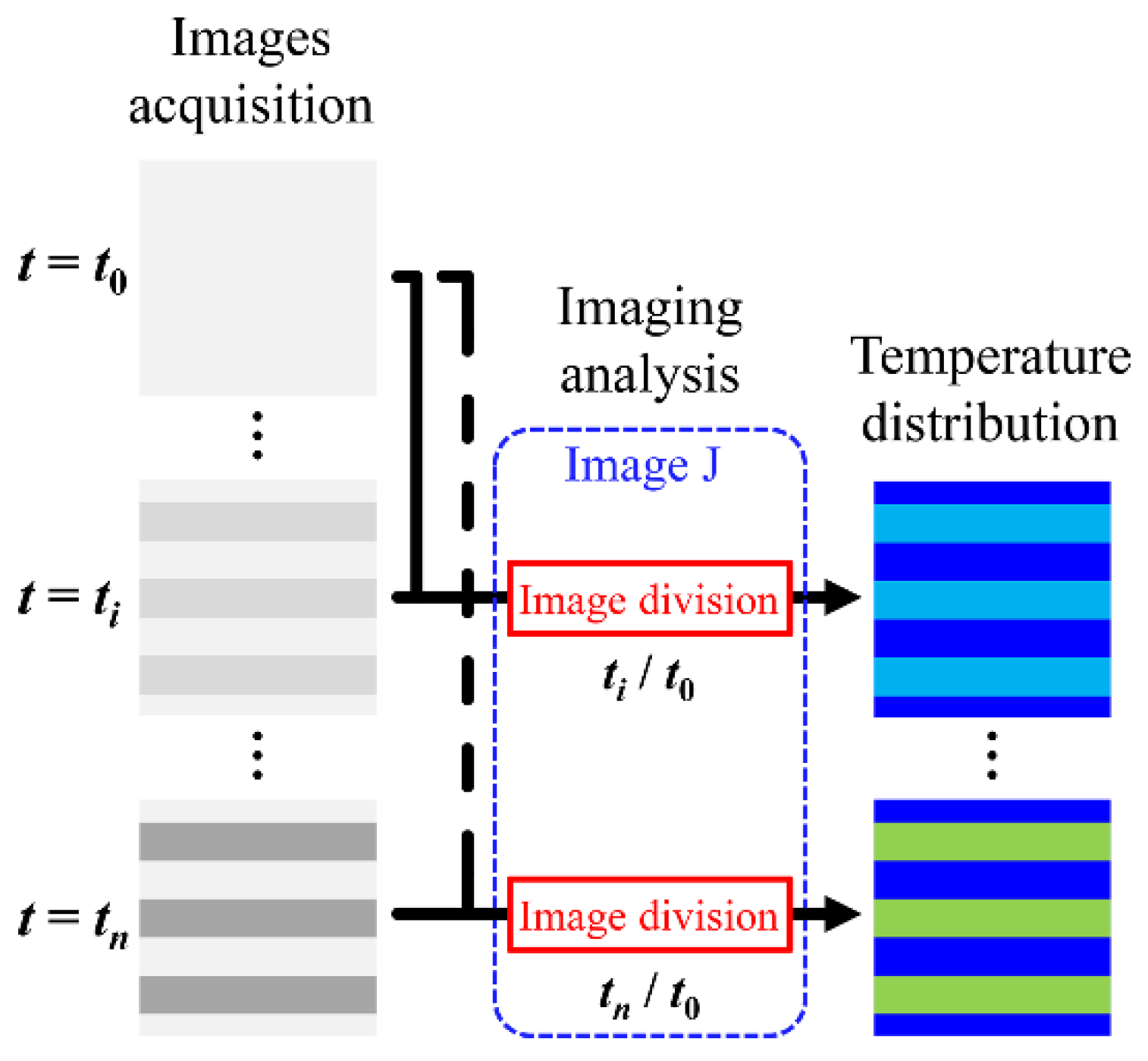
2.5. Image Processing

The procedure for converting the acquired fluorescence images into images of the distribution of the temperature rise $\Delta T$ is shown in Figure 4. The NIH (National Institutes of Health) open-source image-processing software Image J (https://imagej.nih.gov/ij/ accessed on 1 July 2022) was used for image analysis. Time-lapse images of the acquired fluorescence images were sequentially read by Image J and converted into images of the fluorescence intensity ratio by dividing each read image by the reference image acquired before the field application. The converted images were then converted to 8-bit (256 shades of grey scale) text images and the intensity values per image pixel were converted to $\Delta T$ values using the calibration curve. Finally, the distribution of $\Delta T$ was visualized in pseudo-color using the graphical drawing software Tecplot (https://www.tecplot.com/ accessed on 1 July 2022).

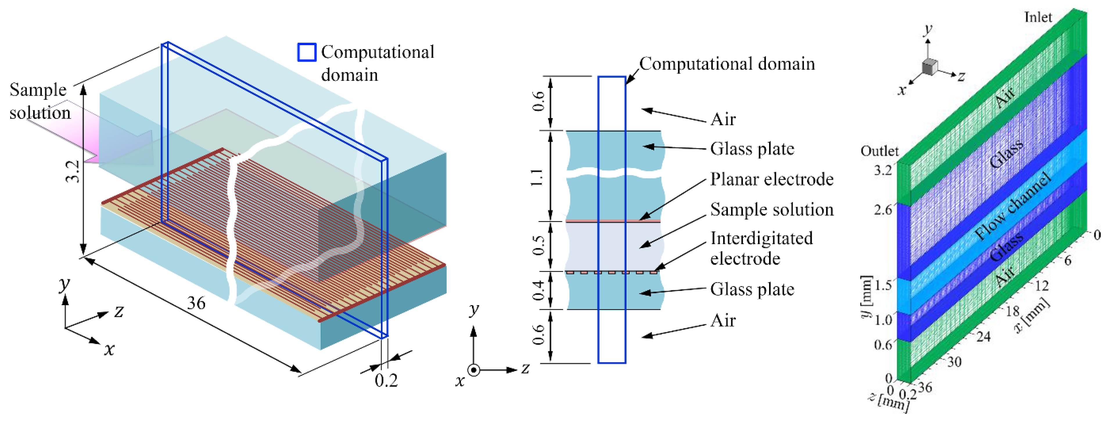
3. Numerical Simulation

Numerical simulations were performed to predict the temperature rise in the device. The numerical simulation model is shown in Figure 5 together with the computational grid. The dimension of the computational domain was 3.2 (height) × 36 (length) × 0.2 (width) mm. The thickness of the interdigitated electrode was ignored for simplicity. The symmetry boundary condition was applied to both the lateral faces (parallel to the $x$-$y$ plane) of the computational domain. In modeling the phenomenon, the effect of natural convection was ignored because the order of the magnitude of the Rayleigh number, $\mathrm{Ra}$, in this phenomenon was $\mathrm{Ra}<~1$. Therefore, it was also approximated that no flows were present in the air layers below and above the bottom and top glass plates, respectively. Consequently, the temperature field could be solved independently of the solution for the flow field. For governing equations, the solution of the fully developed Poiseuille flow

$$v=\left(-\frac{6U}{ \left(y_2-y_1\right) }\left(y-y_1\right)\left(y-y_2\right), 0, 0\right)$$

(2)

was given for the flow velocity vector $v$ using the mean flow velocity $U$, and the time-evolving energy equations for the layers of fluid, glass and air

$$\frac{\partial T}{ \partial t }+\left(v·\mathrm{grad}\right)T=\frac{{\kappa }_w}{ {\rho }_w{C}_p{}_w }\left(\frac{ {\partial }^{2}T }{ \partial x^2}+\frac{ {\partial }^{2}T }{ \partial y^2}+\frac{ {\partial }^{2}T }{ \partial z^2}\right)+\frac{Q}{ {\rho }_w{C}_p{}_w }$$

(3)

$$\frac{\partial T}{ \partial t }=\frac{{\kappa }_g}{ {\rho }_g{C}_p{}_g }\left(\frac{ {\partial }^{2}T }{ \partial x^2}+\frac{ {\partial }^{2}T }{ \partial y^2}+\frac{ {\partial }^{2}T }{ \partial z^2}\right)$$

(4)

$$\frac{\partial T}{ \partial t }=\frac{{\kappa }_a}{ {\rho }_a{C}_p{}_a }\left(\frac{ {\partial }^{2}T }{ \partial x^2}+\frac{ {\partial }^{2}T }{ \partial y^2}+\frac{ {\partial }^{2}T }{ \partial z^2}\right)$$

(5)

were solved simultaneously using the finite difference method. Here, $y_1$ and $y_2$ $\left(y_1<y_2\right)$ are $y$ coordinates of the bottom and top faces of the flow channel; $T$ is temperature; and $\kappa$, $\rho$ and $C_p$ are the thermal conductivity, density and specific heat at constant pressure, respectively. The subscripts $w$, $g$ and $a$ represent values of fluid, glass and air, respectively. Temperatures at the flow inlet and the external boundary of the computational domain were set to 20 °C for boundary conditions for the temperature field. The $\tan \delta$ in Equation (1) of the heat generation term was assumed to have the same functional form of the frequency as [26,27]

$$\tan \delta =2.03\times {10}^7\times f^{-1.48}$$

(6)

For the electric field, $E$, because $E$ is uniform along the flow direction, the Laplace equation for the root mean square value of the electric potential $\Phi$ in the cross-section of the microfluidic channel

$$\frac{ {\partial }^2\Phi }{\partial y^2}+\frac{ {\partial }^2\Phi }{\partial z^2}=0$$

(7)

was solved numerically. The boundary conditions for $\Phi$ were

$$\begin{array}{c}\Phi ={\Phi }_0 \left(\mathrm{High}-\mathrm{voltage} \mathrm{electrodes}\right),\\ \Phi =0 \left(\mathrm{Grounded} \mathrm{electrodes}, \mathrm{top} \mathrm{face} \mathrm{of} \mathrm{the} \mathrm{flow} \mathrm{channel}\right)\end{array}$$

(8)

Boundary conditions for interfaces between the fluid and glass, and between glass and air were

$${ϵ}_w\frac{ \partial \Phi }{\partial n}={ϵ}_g\frac{ \partial \Phi }{\partial n} ,\hspace{1em} {ϵ}_g\frac{ \partial \Phi }{\partial n}={ϵ}_a\frac{ \partial \Phi }{\partial n}$$

(9)

where ${ϵ}_w$, ${ϵ}_g$ and ${ϵ}_a$ are permittivities of the fluid, glass and air, and $n$ is the normal vector at the fluid, glass and air interfaces. For the effective value of the applied voltage, ${\Phi }_0=10/\sqrt{2}$ V was given. The thermophysical properties used in the numerical simulations are listed in

Table 1. Thermophysical properties used in the numerical simulation.

$(\mathbf{a}\mathbf{t} 20 °\mathbf{C})$	$\mathit{\kappa } \left(\mathbf{W}/\mathbf{m} \mathbf{K}\right)$	$\mathit{\rho } \left(\mathbf{k}\mathbf{g}/{\mathbf{m}}^3\right)$	${\mathit{C}}_{\mathit{p}} \left(\mathbf{J}/\mathbf{k}\mathbf{g} \mathbf{K}\right)$	$\mathit{ϵ} \left(\mathbf{F}/\mathbf{m}\right)$
Water	$0.58$	$9.98\times {10}^2$	$4.18\times {10}^3$	$80{ϵ}_0$
Glass	$1.05$	$2.20\times {10}^3$	$0.84\times {10}^3$	$6.0{ϵ}_0$
Air	$2.57\times {10}^{-3}$	$1.17$	$1.01\times {10}^3$	$1.0{ϵ}_0$

. Note that ${ϵ}_0$ in Table 1 is the vacuum permittivity, and the value for water was used for the fluid. Since the temperature rise obtained in the experiment was only a few degrees, values of physical properties were taken at a room temperature of 20 °C. A fully implicit method was implemented to solve the governing equations for temperature. For the computational grid system, the number of hexahedral grid points used was about 1,000,000, and a finer grid with dense grid spacing at the channel inlet and electrode surfaces was adopted. This number of computational grids was the minimum number of grids that would not change (three digits of temperature rise) the results of the simulation. The in-house Fortran parallel-computing code using OpenMP library was used for the numerical simulations. For the numerical simulation of the electric field, Equations (7)–(9) were solved using the Gaussian elimination method. The obtained square of the electric field

$$E^2=E_y{}^2+E_z{}^2={\left(\frac{ \partial \Phi }{\partial y}\right)}^2+{\left(\frac{ \partial \Phi }{\partial z}\right)}^2$$

(10)

was used in the numerical simulation for temperature to evaluate the heat generation in the solution (Equation (1)), where $E_y$ and $E_z$ are $y$ and $z$ components of the electric field, respectively. The in-house Fortran code was also used for the electric potential and field analysis.

4. Results

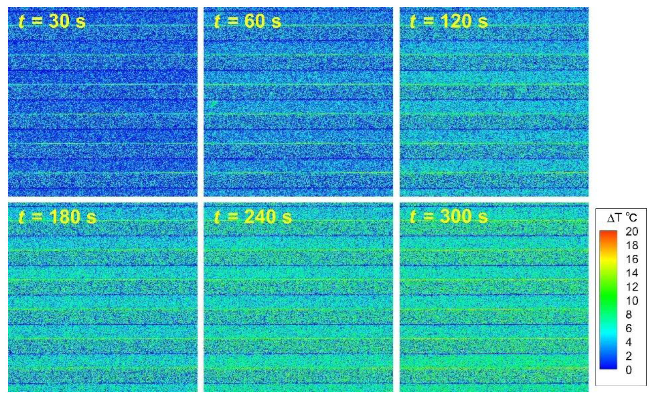
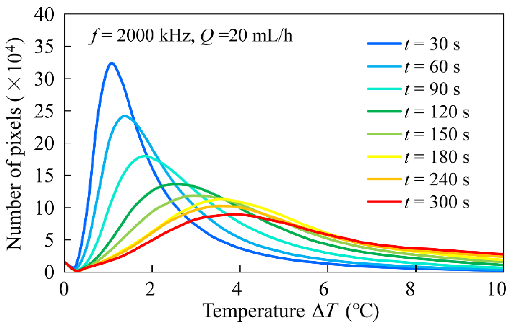
4.1. Distribution of Temperature Rise at the Bottom of the Flow Channel

The time variation in the distribution of the temperature rise, $\Delta T$, at the bottom surface of the flow channel is shown in Figure 6. The image shows the distribution of $\Delta T$ at intervals of 30 s from the onset of the electric-field application to time $t$ = 300 s. The experimental conditions were $f$ = 200 kHz and $Q$ = 5 mL/h. For a while after the field application, there was a noticeable temperature increase at the electrode edge where the electric-field lines concentrated. The temperature of the entire bottom surface of the flow channel also gradually increased with time. The reason for the temperature difference between the electrode surface and the glass surface is thought to be due to the difference in heat capacity. Immediately after the field application, the heat generated at the electrode edge was transferred to both the entire areas of the electrode and the glass substrate by conduction. From the start of the field application to $t~$30 s, the temperature of the aluminum electrode, which has a smaller heat capacity, increased faster than that of the glass, resulting in the difference in distributions of $\Delta T$. However, temperatures of the surfaces of the electrode and glass reached the same level after sufficient time had elapsed, $t~$300 s. It was also observed that the distribution of $\Delta T$ hardly changed in the flow direction. This is because the Reynolds number of the flow so extremely small ($\mathrm{Re}$(=$Uh/\nu$) = 0.14 − 0.56, $U$: mean flow velocity, $h$: flow channel height, $\nu$: dynamic viscosity of water) that $\Delta T$ was hardly affected by convection, and, therefore, the temperature of the electrode surface increased almost uniformly in the flow direction. In other words, the diffusive transport of heat from the electrode surface to the solution was more dominant than the convective transport of heat by the flow of the solution.

4.2. Mean Temperature Rise at the Bottom of the Channel

Image analysis was performed to investigate the distribution of the temperature rise, $\Delta T$, at the bottom of the flow channel in more detail. For this purpose, a histogram of image pixels with values of $\Delta T$ was obtained for each image acquired at each time interval. OpenCV library functions were used to generate the histograms. For each image of the fluorescence intensity ratio before temperature transformation, a non-local mean filter was used to remove noise, after which a histogram of brightness was obtained. Finally, the average value of $\Delta T$ was obtained from the distribution of the obtained histograms. These processes were carried out with Python 3 (ver. 3.9.6, https://www.python.org/ PSF, Wilmington, DE, USA) code. An example of the analysis is shown in Figure 7. The experimental conditions were $f$ = 2000 kHz, $Q$ = 20 mL/h. The histogram curve became broader with time, while the value of $\Delta T$, which gave the maximum, increased. This means that the temperature at the bottom of the flow channel initially increased locally at the electrode surface and soon afterward, the overall temperature increased. It can also be seen that no distinct difference in the temperature appeared between the electrode surface and the glass surface. The histogram was a smooth curve with only a single maximum at each time.

The average of the temperature rise at the bottom of the flow channel, $\Delta T_{av}$, was defined as follows. $\Delta T_{av}$ was obtained by the sum of the multiplication of the temperature rise $\Delta T_i$ ($0\le \Delta T_i\le \Delta T$) with the number of image pixels having the value of the temperature rise $k\left(\Delta T_i\right)$ divided by the total number of image pixels.

$$\Delta T_{av}=\frac{{\sum }_{i=1}^N\Delta T_i·k\left(\Delta T_i\right)}{{\sum }_{i=1}^N k\left(\Delta T_i\right)}$$

(11)

where N is the number of image shades. The resolution of the temperature rise was $\Delta T_{i+1}$−$\Delta T_i$ = 0.26 °C.

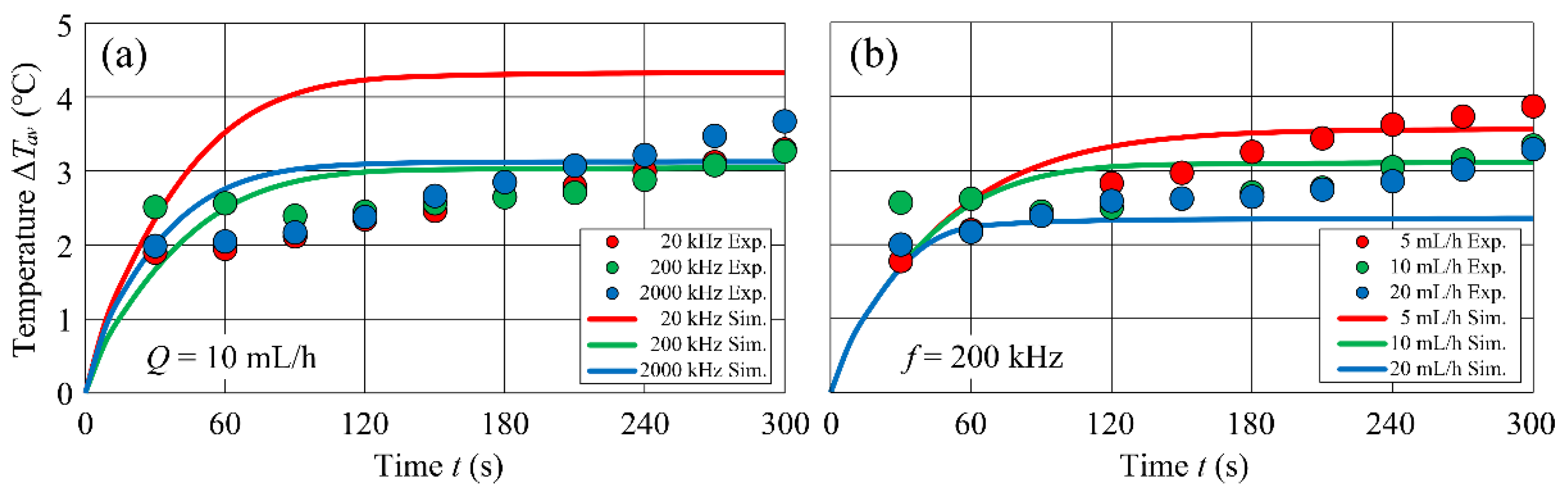
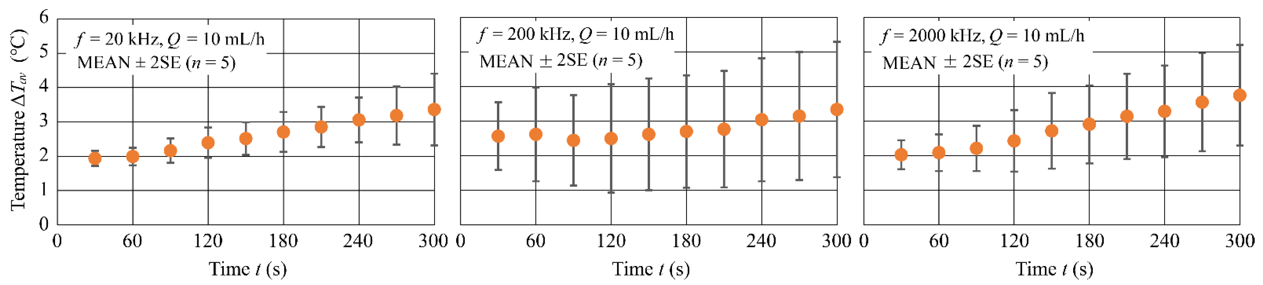
4.3. Dependence of Average Temperature Rise on Frequency

Figure 8 shows the time variation in the average of temperature rise at the bottom of the channel, $\Delta T_{av}$, for three different frequencies, $f$ = 20, 200 and 2000 kHz. The experimental conditions were $V$ = 20 V_pp and $Q$ = 10 mL/h. The data are statistics of five experiments and the plots in the figure are MEAN $\pm$ 2SE. Few differences in $\Delta T_{av}$ according to $f$ appeared, and for all $f$, $\Delta T_{av}$ = $~3$ °C at 300 s after the field application. Results indicate that, at all frequencies, the temperature increased rapidly in the first 30 s and then slowly increased by about 0.7–1.8 °C until 300 s.

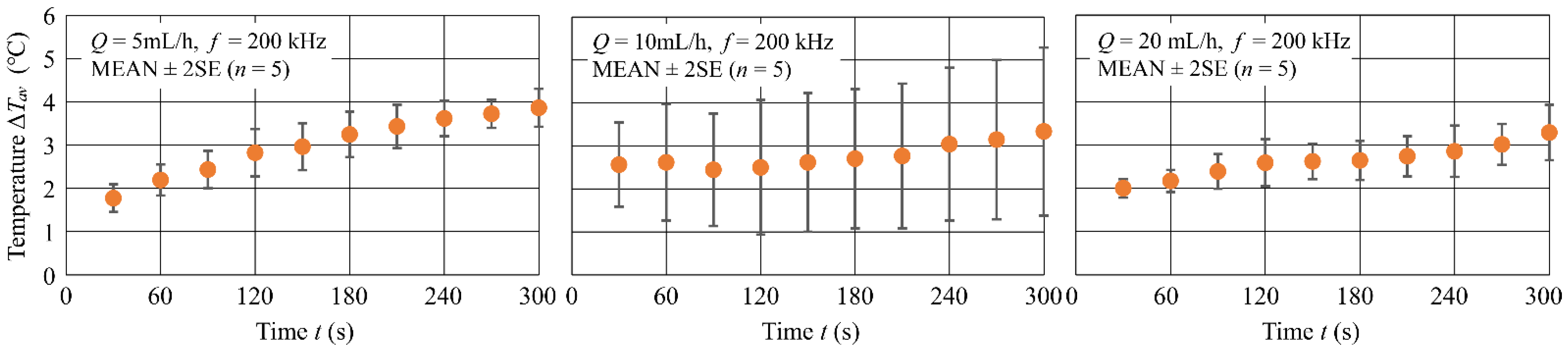
4.4. Dependence of Average Temperature Rise on Flow Rate

Figure 9 shows the time variation of the average temperature rise $\Delta T_{av}$ at the bottom of the flow channel for three different flow rates $Q$ = 5, 10 and 20 mL/h. The experimental conditions were $V$ = 20 V_pp and f = 200 kHz. The data are statistics for five experiments and the plots in the figure are MEAN $\pm$ 2SE. For all values of $Q$, $\Delta T_{av}$ increased with time and reached $\Delta T_{av}$ = 3–4 °C at t = 300 s. In addition, $\Delta T_{av}$ at $t=$ 300 s showed a trend to decrease with increasing $Q$. Results indicate that, at all flow rates, the temperature increased rapidly in the first 30 s and then slowly increased by about 0.7–2.1 °C until 300 s.

4.5. Comparison with Numerical Simulation

Figure 10 shows comparisons of the experimental and numerical simulation results. Figure 10a shows the $f$-dependence of $\Delta T_{av}$ and Figure 10b shows the $Q$-dependence of $\Delta T_{av}$. The plots show the experiments and the solid lines show the numerical simulations. The temperature evaluation position in the numerical simulation was the central part of the microfluidic channel, in accordance with the point of temperature measurement in the experiment.

In the experiment, $\Delta T_{av}$ kept increasing gradually with time, whereas $\Delta T_{av}$ in the numerical simulation generally reached a steady state at $t=$ 90–120 s. The reason for this difference can be attributed to the treatment of thermal boundary conditions in the numerical simulation. The comparison between the numerical simulation and the experiment in Figure 10a shows that they were in general agreement, but for $f$ = 20 kHz, the numerical simulation overestimated the experiment. The comparison between the numerical simulation and the experiment in Figure 10b shows qualitatively good agreement between the two. Comparing the results of the numerical simulations between Figure 10a,b, the time required to reach a steady state of $\Delta T_{av}$ in Figure 10b was clearly reduced by increasing $Q$. Figure 10b also shows that $\Delta T_{av}$ decreased gradually with increasing $Q$ in both experiments and numerical simulations.

5. Discussion

The fraction of electromagnetic energy lost due to the dielectric-loss heat is called dielectric-loss tangent ($\tan \delta$). $\tan \delta$ varies with the AC frequency and the physical properties of dielectric materials. Because the value of $\tan \delta$ decreases with increasing f in the frequency range $f<$ 2000 kHz [28,29,30], it was expected that $\Delta T_{av}$ would also decrease with increasing f. However, the $f$-dependence of $\Delta T_{av}$ did not appear clearly and about $\Delta T_{av}$ = 2–4 °C for any $f$. The reason for this is that the majority of $\Delta T_{av}$ was due to Joule heating because the heating due to the dielectric losses was small. A reduction in the signal-to-noise ratio which occurred when digitizing the fluorescence images is also considered to be a reason for the measurement error. The difference of the transient behaviors of temperature rise between experiment and numerical prediction may be attributed to the treatment of the thermal boundary condition in the numerical simulation model. The boundary condition of the constant temperature at the outer bound of the air layer may not have adequately represented the actual thermal behavior of the device. Another major reason may be that the periodic boundary conditions were applied to both side walls of the computational domain in the numerical simulations. In the actual device, although expected to be slight, there is also heat dissipation on both sides of the microfluidic channel, which might give the very gradual temperature rise.

Comparing numerical simulations and experiments, the $f$-dependence of $\Delta T_{av}$ was overestimated in numerical simulations compared to experiments. The reason for this could be attributed to the accuracy of the $\tan \delta$ model in the low-frequency range. Because the measured data for value of $\tan \delta$ is limited, and within the range of $f$ in the present study, the accuracy is about one order of magnitude. Regarding the $Q$-dependence, $\Delta T_{av}$ gradually decreased with increasing $Q$, and the experimental and numerical simulations agreed qualitatively well. For all values of $Q$, the $\Delta T_{av}$ reached was $~$3–4 °C at t = 300 s. Looking at $\Delta T_{av}$ after 300 s from the field application, the decrease in $\Delta T_{av}$ was about $\Delta T_{av}$ = 0.7 °C. When compared with the change in the value of $Q$ from $Q$ = 5 mL/h to $Q$ = 20 mL/h, the rate of decrease in $\Delta T_{av}$ was small. The reason for this may be that the cooling effect of forced convection heat transport is insufficient due to the small Reynolds number of the flow.

Although a significant increase in $Q$ can be expected to reduce the temperature increase in the device, this is likely to reduce the cell separation ratio of the device due to the increased hydrodynamic resistance force acting on the cells. In other words, increasing the flow rate in cell separation devices often significantly reduces the performance of the device and is unlikely to have the desired effect. The best way to keep the temperature rise to a minimum without affecting the cell separation rate is to use a low-conductivity suspension and flow the cell sample through the device at a moderate flow rate.

In summary, the temperature rise obtained in this study ranged from 2 to 4 °C. This value suggests that even when cell separation is performed at, for example, body temperature of 37 °C, the temperature inside the device is, at most, estimated to be about $~$41 °C, and the temperature affecting the cells [10] is not reached.

6. Conclusions

Temperature field analysis was performed to investigate the temperature rise in cell separation devices using AC-electric-field-induced dielectrophoresis. The temperature rise at the bottom of the flow channel in the device was measured using the laser-induced fluorescence (LIF) method, and numerical simulations of the heat and fluid flow were performed using the energy equations considering the generation of Joule heat and the dielectric-loss heat in the solution exposed to the electric field.

No clear frequency dependence was observed in the temperature rise, with an average temperature rise of about 2–4 °C at 300 s after the onset of the electric-field application. The reason for this could be that the majority of the temperature rise was due to the frequency-independent Joule heating, because the heating due to dielectric losses was small. Numerical simulations overestimated the experimental results in the low-frequency range. A possible reason for this is the accuracy of the heat generation model in the low-frequency range. Regarding the dependence of the temperature rise on flow rate, the temperature rise decreased gradually with increasing flow rate and the average temperature rise was about 3–4 °C at 300 s after the onset of the field application. Experimental and numerical simulations also agreed qualitatively well.

When cell separation was performed with the developed device, the average temperature rise in the device was about 2–4 °C after 300 s of continuous operation, which suggests that the effect on cells is small when using solutions with low conductivity ($\sigma$ = 1 mS/m). In recent years, there has been a growing trend toward the usage of higher voltages to increase separation efficiency, and the use of high-conductivity solutions to reduce damage to cells. However, both of these factors can easily lead to a significant temperature increase in the device. In this study, it was shown that short-time ($~$300 s) processing with low-conductivity solutions not only achieves high separation efficiency [17], but also keeps the temperature rise in the device low. While the use of low-conductivity solutions can suppress the temperature rise in the device, the adverse effect on cell viability is significant when the time of the device operation is longer than 30 min (unpublished data). Further study is needed to find a method that can process a large number of cells in a shorter time.

References

1. Kung, Y.; Niazi, K.R.; Chiou, P. Tunnel dielectrophoresis for ultra-high precision size-based cell separation. Lab Chip 2021, 21, 1049–1060. [Google Scholar] [CrossRef]
2. Shirmohammadli, V.; Manavizadeh, N. Application of differential electrodes in a dielectrophoresis-based device for cell separation. IEEE Trans. Electron Devices 2019, 66, 4075–4080. [Google Scholar] [CrossRef]
3. Shen, S.; Yi, Z.; Li, X.; Xie, S.; Jin, M.; Zhou, G.; Yan, Z.; Shui, L. Flow-field-assisted dielectrophoretic microchips for high-efficiency sheathless particle/cell separation with dual mode. Anal. Chem. 2021, 93, 7606–7615. [Google Scholar] [CrossRef]
4. Jones, T.B. Electromechanics of Particles; Cambridge University Press: Cambridge, UK, 1995. [Google Scholar]
5. Rahmati, M.; Chen, X. Separation of circulating tumor cells from blood using dielectrophoretic DLD manipulation. Biomed. Microdevices 2021, 23, 49. [Google Scholar] [CrossRef] [PubMed]
6. Saydé, T.; Manczak, R.; Saada, S.; Bégaud, G.; Bessette, B.; Lespes, G.; Coustumer, P.L.; Gaudin, K.; Dalmay, C.; Pothier, A.; et al. Characterization of glioblastoma cancer stem cells sorted by sedimentation field-flow fractionation using an ultrahigh-frequency range dielectrophoresis biosensor. Anal. Chem. 2021, 93, 12664–12671. [Google Scholar] [CrossRef] [PubMed]
7. Oh, M.; Jayasooriya, V.; Woo, S.O.; Nawarathna, D.; Choi, Y. Selective manipulation of biomolecules with insulator-based dielectrophoretic tweezers. ACS Appl. Nano Mater. 2020, 3, 797–805. [Google Scholar] [CrossRef] [PubMed] [Green Version]
8. Zhang, J.; Song, Z.; Liu, Q.; Song, Y. Recent advances in dielectrophoresis-based cell viability assessment. Electrophoresis 2020, 41, 917–932. [Google Scholar] [CrossRef]
9. Metaxas, A.C.; Meredith, R.J. Industrial Microwave Heating; Institution of Engineering and Technology: London, UK, 1988. [Google Scholar]
10. Samalia, A.; Holmberg, C.I.; Sistonen, L.; Orrenius, S. Thermotolerance and cell death are distinct cellular responses to stress: Dependence on heat shock proteins. FEBS Lett. 1999, 461, 306–310. [Google Scholar] [CrossRef] [Green Version]
11. Reissis, Y.; García-Gareta, E.; Korda, M.; Blunn, G.W.; Hua, J. The effect of temperature on the viability of human mesenchymal stem cells. Stem Cell Res. Ther. 2013, 4, 139. [Google Scholar] [CrossRef] [Green Version]
12. Tay, F.E.H.; Yu, L.; Panga, A.J.; Iliescu, C. Electrical and thermal characterization of a dielectrophoretic chip with 3D electrodes for cells manipulation. Electrochim. Acta 2007, 52, 2862–2868. [Google Scholar] [CrossRef]
13. Sridharan, S.; Zhu, J.; Hu, G.; Xuan, X. Joule heating effects on electroosmotic flow in insulator-based dielectrophoresis. Electrophoresis 2011, 32, 2274–2281. [Google Scholar] [CrossRef] [PubMed] [Green Version]
14. Kale, A.; Patel, S.; Qian, S.; Hu, G.; Xuan, X. Joule heating effects on reservoir-based dielectrophoresis. Electrophoresis 2014, 35, 721–727. [Google Scholar] [CrossRef] [Green Version]
15. Nakano, A.; Luo, J.; Ros, A. Temporal and spatial temperature measurement in insulator-based dielectrophoretic devices. Anal. Chem. 2014, 86, 6516–6524. [Google Scholar] [CrossRef] [Green Version]
16. Kwak, T.J.; Hossen, I.; Bashir, R.; Chang, W.; Lee, C.H. Localized dielectric loss heating in dielectrophoresis devices. Sci. Rep. 2019, 9, 18977. [Google Scholar] [CrossRef] [Green Version]
17. Seki, Y.; Nagasaka, A.; Gondo, T.; Tada, S.; Eguchi, M. Continuous separation of biological cells using a new type of dielectrophoresis-based microfluidic device. In Proceedings of the SB3C2022 Summer Biomechanics, Bioengineering and Biotransport Conference, Eastern Shore, MD, USA, 20–23 June 2022; p. 173. [Google Scholar]
18. Shah, J.J.; Gaitan, M.; Geist, J. Generalized temperature measurement equations for rhodamine B dye solution and its application to microfluidics. Anal. Chem. 2009, 81, 8260–8263. [Google Scholar] [CrossRef]
19. Glawdel, T.; Almutairi, Z.; Wang, S.; Ren, C. Photobleaching absorbed rhodamine B to improve temperature measurements in PDMS microchannels. Lab Chip 2009, 9, 171–174. [Google Scholar] [CrossRef]
20. Puri, P.; Kumar, V.; Belgamwar, S.U.; Ananthasubramanian, M.; Sharma, N.N. Microfluidic platform for dielectrophoretic separation of bio-particles using serpentine microelectrodes. Microsyst. Technol. 2019, 25, 2813–2820. [Google Scholar] [CrossRef]
21. Nie, X.; Luo, Y.; Shen, P.; Han, C.; Yu, D.; Xing, X. High-throughput dielectrophoretic cell sorting assisted by cell sliding on scalable electrode tracks made of conducting-PDMS. Sens. Actuators B Chem. 2021, 327, 128873. [Google Scholar] [CrossRef]
22. Mishra, Y.N.; Yoganantham, A.; Koegl, M.; Zigan, L. Investigation of five organic dyes in ethanol and butanol for two-color laser-induced fluorescence ratio thermometry. Optics 2020, 1, 1–17. [Google Scholar] [CrossRef] [Green Version]
23. Piskunov, M.V.; Strizhak, P.A. Using planar laser induced fluorescence to explain the mechanism of heterogeneous water droplet boiling and explosive breakup. Exp. Therm. Fluid Sci. 2018, 91, 103–116. [Google Scholar] [CrossRef]
24. Tada, S. Numerical simulation of dielectrophoretic separation of live/dead cells using a three-dimensional nonuniform AC electric field in micro-fabricated devices. Biorheology 2015, 52, 211–224. [Google Scholar] [CrossRef]
25. Puri, P.; Kumar, V.; Belgamwar, S.U.; Sharma, N.N. Microfluidic device for cell trapping with carbon electrodes using dielectrophoresis. Biomed. Microdevices 2018, 20, 102. [Google Scholar] [CrossRef] [PubMed]
26. Midi, N.S.; Sasaki, K.; Ohyama, R.; Shinyashiki, N. Broadband complex dielectric constants of water and sodium chloride aqueous solutions with different DC conductivities, IEEJ Trans. Electr. Electron. Eng. 2014, 9, S8–S12. [Google Scholar]
27. Gómez-Galván, F.; Lara-Ceniceros, T.; Mercado-Uribe, H. Device for simultaneous measurements of the optical and dielectric properties of hydrogels. Meas. Sci. Technol. 2012, 23, 025602. [Google Scholar] [CrossRef]
28. Shayegani Akmal, A.A.; Borsi, H.; Gockenbach, E.; Wasserberg, V.; Mohseni, H. Dielectric behavior of insulating liquids at very low frequency. IEEE Trans. Dielectr. Electr. Insul. 2006, 13, 532–538. [Google Scholar] [CrossRef]
29. Rander, D.N.; Joshi, Y.S.; Kanse, K.S.; Kumbharkhane, A.C. Dielectric dispersion and hydrogen bonding interactions study of aqueous D-mannitol using time domain reflectometry. Phys. Chem. Liquids 2015, 53, 187–192. [Google Scholar] [CrossRef]
30. Zhang, C.; Hou, Z.; Zhang, B.; Fang, H.; Bi, S. High sensitivity self-recovery ethanol sensor based on polyporous graphene oxide/melamine composites. Carbon 2018, 137, 467–474. [Google Scholar] [CrossRef]
Figure 1. Schematics of (a) the cell separation device and (b) the counter-interdigitated electrode substrate.
Fluids 07 00263 g001
Figure 2. Experimental setup.
Fluids 07 00263 g002
Figure 3. Temperature calibration curve.
Fluids 07 00263 g003
Figure 4. Procedure for converting the fluorescence images into images of the distribution of ΔT.
Fluids 07 00263 g004
Figure 5. Numerical simulation model and computational grid.
Fluids 07 00263 g005
Figure 6. Time variation in the distribution of Δ T at the bottom surface of the flow channel.
Fluids 07 00263 g006
Figure 7. An example of image analysis of the distribution of Δ T .
Fluids 07 00263 g007
Figure 8. Time variation in Δ T a v for three different values of frequency.
Fluids 07 00263 g008
Figure 9. Time variation in Δ T a v for three different values of flow rate.
Fluids 07 00263 g009
Figure 10. Comparisons of the experimental and numerical simulation results.
Fluids 07 00263 g010