Single Contaminated Drops Falling through Stagnant Liquid at Low Reynolds Numbers

Abstract

Numerical simulations of contaminated spherical drops falling through a stagnant liquid at low Reynolds numbers are carried out using the finite difference method. The numerical results are used to describe the behavior of the surfactant concentrations and to understand the surfactant effects on the fluid motions in detail. The predicted interfacial surfactant concentration, $\mathsf{\Gamma }$, is almost zero for angles, $\theta$, below a certain value (the stagnant-cap angle, ${\theta }_{cap}$), whereas it steeply increases and reaches a large value for $\theta >{\theta }_{cap}$ (the stagnant-cap region). The increase in the initial surfactant concentration, $C_0$, in the drop enhances the adsorption from the drop to the interface, which results in the increase in $\mathsf{\Gamma }$ and the decrease in ${\theta }_{cap}$. Peaks appear in the predicted Marangoni stresses around ${\theta }_{cap}$, which causes similar peaks in the pressure distribution. The high-pressure spots prevent the fluid motion along the interface, which results in the formation of the stagnant-cap region and the attenuation of the tangential velocity in the continuous phase. The surfactant flux from the bulk to the interface decreases C in the vicinity of the interface for $\theta <{\theta }_{cap}$ and the weak diffusion cannot compensate for the reduction in C by adsorption, which results in C at the interface smaller than $C_0$. The pattern of the low C region is determined by the advection and does not smear out because of a small diffusive flux.

1. Introduction

Surface-active agents (surfactants) have various effects on the motion of a fluid particle, e.g., the drag coefficient of a spherical bubble under a fully contaminated condition corresponds to that of a solid particle [1,2], capillary waves formed on the surface of a bubble are dampened by the presence of surfactant [3,4], and so on. Boussinesq [5] assumed that the interface contaminated with surfactant behaves similar to a viscous membrane and modeled the increase in drag caused by the presence of surfactant as surface viscosity [1,6]. The drag model for clean spherical fluid particles of low Reynolds numbers, i.e., the Hadamard–Rybczynski model [7,8], can be easily extended to that for contaminated fluid particles by introducing the surface viscosity. On the other hand, Levich [9] succeeded in explaining the surfactant effect on the drag force by accounting for the surface tension gradient, i.e., the Marangoni stress, caused by non-uniform distribution of the surface tension due to the adsorption of surfactant to the interface. Numerical simulations of contaminated fluid particles have been carried out so far by taking into account the Marangoni stress [2,10,11,12,13,14,15,16,17,18,19,20], in contrast, measurements of the Marangoni stress and the interfacial surfactant concentration have rarely been carried out.

Reduction in the surface tension due to surfactant adsorption takes place for various surfactants such as Triton X-100, sodium dodecyl sulfate (SDS), alcohols such as 1-pentanol and so on. In the presence of interfacial flow, the distribution of surfactant at the interface is non-uniform due to advection. For example, the interfacial flow formed at the interface of a drop falling through a stagnant liquid due to gravity transfers surfactant molecules adsorbing to the interface from the nose side to the rear side of the drop, which results in a high surfactant concentration in the rear side. The non-uniform surfactant distribution also results in a non-uniform distribution of surface tension. The distribution of the surface tension can be calculated if the Marangoni stress is measured, and the interfacial surfactant concentration can also be computed from the surface tension by making use of the Langmuir–Szyszkowski isotherm [21]. The Marangoni stress can be evaluated if the velocity gradients at the interface and the viscosities of the two phases are known since the jump of the tangential viscous stress at the interface balances with the Marangoni stress. Hosokawa et al. [22] measured velocity fields about single contaminated drops of a glycerol–water solution falling through a silicone oil at low drop Reynolds numbers using SFV (spatiotemporal filter velocimetry) [23] to evaluate the distributions of the interfacial surfactant concentration (Figure 1). However, other field variables, e.g., the surfactant concentration in the drop and the pressure fields, required for full understanding of the phenomena, have not been obtained in the experiment yet.

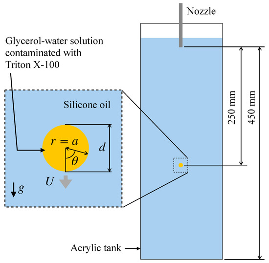
Figure 1. Single drop falling through stagnant liquid [22], where d is the drop diameter, a is the drop radius, r and $\theta$ are the radial and azimuthal coordinates, U is the drop velocity, and g is the magnitude of the gravitational acceleration.

In this study, the motions of contaminated drops of low Reynolds numbers are numerically simulated using the finite difference method under the same conditions as those in Hosokawa et al. [22] to discuss the distributions of the bulk and interfacial surfactant concentrations and the surfactant effects on the interface velocity and pressure in detail. In the following sections, the numerical method is first introduced. The validity of the numerical method is examined for clean drops, spherical particles and contaminated bubbles [10]. Then, the falling motions of contaminated drops are simulated, and the surfactant effects are discussed.

2. Numerical Method

2.1. Governing Equations

The governing equations are written in the frame of reference moving with a single drop. The drop shape is assumed to be spherical, and the drop Reynolds number is given as a parameter from the experimental data [22]. The flow passing through the spherical drop at the prescribed Reynolds number is therefore obtained by solving the governing equations. The $(r,\theta )$ two-dimensional spherical coordinates are used since the flow has axial symmetry at low drop Reynolds numbers. The flow is assumed to be incompressible and isothermal. The Navier–Stokes equation for Newtonian fluids is therefore given by [24]

$${\rho }_k\left(\frac{\partial u_{r,k}}{\partial t}+{\mathbf{u}}_k·\nabla u_{r,k}-\frac{u_{\theta ,k}^2}{r}\right)=-\frac{\partial p_k}{\partial r}+{\mu }_k\left({\nabla }^2{u}_{r,k}-\frac{2u_{r,k}}{r^2}-\frac{2}{r^{2}sin\theta }\frac{\partial sin\theta u_{\theta ,k}}{\partial \theta }\right)$$

(1)

$${\rho }_k\left(\frac{\partial u_{\theta ,k}}{\partial t}+{\mathbf{u}}_k·\nabla u_{\theta ,k}+\frac{u_{r,k}{u}_{\theta ,k}}{r}\right)=-\frac{1}{r}\frac{\partial p_k}{\partial \theta }+{\mu }_k\left({\nabla }^2{u}_{\theta ,k}+\frac{2}{r^2}\frac{\partial u_{r,k}}{\partial \theta }-\frac{u_{\theta ,k}}{r^2{sin}^2\theta }\right)$$

(2)

where $u_r$ and $u_{\theta }$ are the velocity components in the r and $\theta$ directions, respectively, t is the time, p is the pressure, $\rho$ is the density, $\mu$ is the viscosity, and k denotes either the dispersed phase ($k=D$) or the continuous phase ($k=C$). The differential operators, $\mathbf{u}·\nabla$ and ${\nabla }^2$, are given in Appendix A. The following continuity equation holds in each phase:

$$\frac{1}{r^2}\frac{\partial }{\partial r}\left(r^2\frac{\partial u_{r,k}}{\partial r}\right)+\frac{1}{rsin\theta }\frac{\partial (sin\theta u_{\theta ,k})}{\partial \theta }=0$$

(3)

The normal component of the velocity is continuous at the interface when there is no interfacial mass transfer. Hence the velocity boundary condition at the drop interface is given by

$$u_{r,D}=u_{r,C}=0$$

(4)

and the following no-slip condition is used for the tangential velocity component:

$$u_{\theta ,D}=u_{\theta ,C}=u_{\theta ,int}$$

(5)

where the subscript $int$ denotes the interface. The tangential viscous stress, ${\tau }_{r\theta }$, in each phase balances with the Marangoni stress at the interface:

$${\left[{\tau }_{r\theta }\right]}_{int}=\frac{1}{a}\frac{\partial \sigma }{\partial \theta }$$

(6)

where ${\left[X\right]}_{int}$ represents the jump of the quantity, X, at the interface, $\sigma$ is the surface tension, and a is the drop radius.

In the present study, surfactant is assumed to be soluble in the dispersed phase, so that it is present inside the drop at the molar concentration, C. The transport equation of C is given by

$$\frac{\partial C}{\partial t}+\nabla ·{\mathbf{u}}_{D}C=\nabla ·D_D\nabla C$$

(7)

where $D_D$ is the diffusion coefficient. Adsorption and desorption of surfactant molecules take place at the interface and the magnitude of the adsorption–desorption flux depends on C at the interface, $C_S$, and the molar concentration, $\mathsf{\Gamma }$, of surfactant adsorbing to the interface. The transport equation of $\mathsf{\Gamma }$ is given by [2,10,25]

$$\frac{\partial \mathsf{\Gamma }}{\partial t}+{\nabla }_S·{\mathbf{u}}_S\mathsf{\Gamma }={\nabla }_S·D_S{\nabla }_S\mathsf{\Gamma }+{\dot{S}}_{\mathsf{\Gamma }}$$

(8)

where $D_S$ is the diffusion coefficient of surfactant at the interface, ${\nabla }_S$ is the surface gradient operator, and ${\mathbf{u}}_S$ is the interface velocity. The ${\dot{S}}_{\mathsf{\Gamma }}$ is the net adsorption–desorption flux, which is evaluated by making use of the following Frumkin–Levich model [9,10,26]:

$${\dot{S}}_{\mathsf{\Gamma }}=k_a{C}_S({\mathsf{\Gamma }}_{max}-\mathsf{\Gamma })-k_d\mathsf{\Gamma }$$

(9)

where $k_a$ is the adsorption rate constant, $k_d$ is the desorption rate constant, and ${\mathsf{\Gamma }}_{max}$ is the saturation value of $\mathsf{\Gamma }$. The diffusive flux of C at the interface balances with ${\dot{S}}_{\mathsf{\Gamma }}$, i.e.,

$$-D_D{\left.\frac{\partial C}{\partial r}\right|}_{r=a}={\dot{S}}_{\mathsf{\Gamma }}$$

(10)

The surface tension, $\sigma$, of the contaminated interface depends on $\mathsf{\Gamma }$ as [21]

$$\sigma ={\sigma }_0+R_{G}T{\mathsf{\Gamma }}_{max}ln\left(1-\frac{\mathsf{\Gamma }}{{\mathsf{\Gamma }}_{max}}\right)$$

(11)

where ${\sigma }_0$ is the surface tension of a clean interface, $R_G$ is the universal gas constant, and T is the temperature.

The following dimensionless forms of the governing equations are useful to make clear the relevant dimensionless groups:

$$\frac{\partial u_{r,k}^{\ast }}{\partial t^{\ast }}+{\mathbf{u}}_k^{\ast }·{\nabla }^{\ast }{u}_{r,k}^{\ast }-\frac{u_{\theta ,k}^{\ast 2}}{r^{\ast }}=-\frac{\partial p_k^{\ast }}{\partial r^{\ast }}+\frac{1}{R{e}_k}\left[{\nabla }^{\ast 2}{u}_{r,k}^{\ast }-\frac{2u_{r,k}^{\ast }}{r^{\ast 2}}-\frac{2}{r^{\ast 2}sin\theta }\frac{\partial sin\theta u_{\theta ,k}^{\ast }}{\partial \theta }\right]$$

(12)

$$\frac{\partial u_{\theta ,k}^{\ast }}{\partial t^{\ast }}+{\mathbf{u}}_k^{\ast }·\nabla u_{\theta ,k}^{\ast }+\frac{u_{r,k}^{\ast }{u}_{\theta ,k}^{\ast }}{r^{\ast }}=-\frac{1}{r^{\ast }}\frac{\partial p_k^{\ast }}{\partial \theta }+\frac{1}{R{e}_k}\left[{\nabla }^{\ast 2}{u}_{\theta ,k}^{\ast }+\frac{2}{r^{\ast 2}}\frac{\partial u_{r,k}^{\ast }}{\partial \theta }-\frac{u_{\theta ,k}^{\ast }}{r^{\ast 2}{sin}^2\theta }\right]$$

(13)

$$\frac{\partial C^{\ast }}{\partial t^{\ast }}+{\nabla }^{\ast }·{\mathbf{u}}_D^{\ast }{C}^{\ast }=\frac{{\nabla }^{\ast 2}{C}^{\ast }}{P{e}_D}$$

(14)

$$\frac{\partial {\mathsf{\Gamma }}^{\ast }}{\partial t^{\ast }}+{\nabla }_S^{\ast }·{\mathbf{u}}_S^{\ast }{\mathsf{\Gamma }}^{\ast }=\frac{{\nabla }_S^{\ast 2}{\mathsf{\Gamma }}^{\ast }}{P{e}_S}+{\dot{S}}_{\mathsf{\Gamma }}^{\ast }$$

(15)

where ${\mathbf{u}}^{\ast }=\mathbf{u}/U$, $p^{\ast }=p/\rho U^2$, $C^{\ast }=C/C_0$, ${\mathsf{\Gamma }}^{\ast }=\mathsf{\Gamma }/{\mathsf{\Gamma }}_{max}$, $r^{\ast }=r/d$, $t^{\ast }=Ut/d$, ${\nabla }^{\ast }=d\nabla$, ${\nabla }_S^{\ast }=d{\nabla }_S$, and $C_0$ is the initial concentration. The Reynolds numbers, $R{e}_k$, the Peclet number, $P{e}_D$, and the surface Peclet number, $P{e}_S$, are defined by $R{e}_k={\rho }_{k}Ud/{\mu }_k$, $P{e}_D=Ud/D_D$, and $P{e}_S=Ud/D_S$, respectively, where d is the drop diameter, and U is the drop velocity. The momentum jump condition in the tangential direction is given by

$${\left[{\tau }_{r\theta }^{\ast }\right]}_{int}=\frac{Ma}{a^{\ast }}\frac{\partial {\sigma }^{\ast }}{\partial \theta }$$

(16)

where the Marangoni number, $Ma$, and the dimensionless surface tension, ${\sigma }^{\ast }$, are defined by $Ma=R_{G}T{\mathsf{\Gamma }}_{max}/{\mu }_{C}U$ and ${\sigma }^{\ast }=\sigma /R_{G}T{\mathsf{\Gamma }}_{max}$, respectively. The dimensionless radius is given by $a^{\ast }=a/d=1/2$. The interfacial surfactant flux in the dimensionless form is given by

$${\dot{S}}_{\mathsf{\Gamma }}^{\ast }=\alpha \left[C_S^{\ast }(1-{\mathsf{\Gamma }}^{\ast })-\frac{{\mathsf{\Gamma }}^{\ast }}{La}\right]$$

(17)

where $C_S^{\ast }=C_S/C_0$, $La$ is the Langmuir number defined by $La=k_a{C}_0/k_d$, and $\alpha$ is the ratio of the adsorption rate to the characteristic velocity, i.e., $\alpha =k_a{C}_{0}d/U$. The boundary condition of C at the interface is

$$-{\left.\frac{\partial C^{\ast }}{\partial r^{\ast }}\right|}_{r^{\ast }=a^{\ast }}=P{e}_{D}K{\dot{S}}_{\mathsf{\Gamma }}^{\ast }$$

(18)

where K is the dimensionless adsorption length defined by $K={\mathsf{\Gamma }}_{max}/C_{0}d$. The ${\sigma }^{\ast }$ is given by

$${\sigma }^{\ast }={\sigma }_0^{\ast }+ln(1-{\mathsf{\Gamma }}^{\ast })$$

(19)

where ${\sigma }_0^{\ast }={\sigma }_0/R_{G}T{\mathsf{\Gamma }}_{max}$.

2.2. Discretization Schemes

2.2.1. Velocity-Pressure Coupling

The present numerical method for obtaining the velocity and pressure fields is based on the fractional step method [27,28]. The Adams–Bashforth scheme is used for the advection terms of the Navier–Stokes equations, while the Crank–Nicolson scheme is used for the diffusion terms. Therefore,

$$\begin{array}{cc}\hfill & {\nabla }^{\ast 2}{u}_{r,k}^{\ast m}-\frac{2u_{r,k}^{\ast m}}{r^{\ast 2}}-\frac{2R{e}_k}{\Delta t^{\ast }}{u}_{r,k}^{\ast m}-\frac{2}{r^{\ast 2}sin\theta }\frac{\partial sin\theta u_{\theta ,k}^{\ast m-1}}{\partial \theta }=S_{r,k}\hfill \end{array}$$

(20)

$$\begin{array}{cc}\hfill & {\nabla }^{\ast 2}{u}_{\theta ,k}^{\ast m}-\frac{u_{\theta ,k}^{\ast m}}{r^{\ast 2}{sin}^2\theta }-\frac{2R{e}_k}{\Delta t^{\ast }}{u}_{\theta ,k}^{\ast m}+\frac{2}{r^{\ast 2}}\frac{\partial u_{r,k}^{\ast m-1}}{\partial \theta }=S_{\theta ,k}\hfill \end{array}$$

(21)

where $\Delta t^{\ast }$ is the time step size and

$$\begin{array}{cc}\hfill & S_{r,k}=-D_{r,k}^n+2R{e}_k\left[-\frac{u_{r,k}^{\ast n}}{\Delta t^{\ast }}+\frac{3A_{r,k}^n-A_{r,k}^{n-1}}{2}+\frac{\partial p_k^{\ast n}}{\partial r^{\ast }}\right]\hfill \end{array}$$

(22)

$$\begin{array}{cc}\hfill & D_{r,k}={\nabla }^{\ast 2}{u}_{r,k}^{\ast }-\frac{2u_{r,k}^{\ast }}{r^{\ast 2}}-\frac{2}{r^{\ast 2}sin\theta }\frac{\partial sin\theta u_{\theta ,k}^{\ast }}{\partial \theta }\hfill \end{array}$$

(23)

$$\begin{array}{cc}\hfill & A_{r,k}={\mathbf{u}}_k^{\ast }·{\nabla }^{\ast }{u}_{r,k}^{\ast }-\frac{u_{\theta ,k}^{\ast 2}}{r^{\ast }}\hfill \end{array}$$

(24)

$$\begin{array}{cc}\hfill & S_{\theta ,k}=-D_{\theta ,k}^n+2R{e}_k\left[-\frac{u_{\theta ,k}^{\ast n}}{\Delta t^{\ast }}+\frac{3A_{\theta ,k}^n-A_{\theta ,k}^{n-1}}{2}+\frac{1}{r^{\ast }}\frac{\partial p_k^{\ast n}}{\partial \theta }\right]\hfill \end{array}$$

(25)

$$\begin{array}{cc}\hfill & D_{\theta ,k}={\nabla }^2{u}_{\theta ,k}^{\ast }+\frac{2}{r^{\ast 2}}\frac{\partial u_{r,k}^{\ast }}{\partial \theta }-\frac{u_{\theta ,k}^{\ast }}{r^{\ast 2}{sin}^2\theta }\hfill \end{array}$$

(26)

$$\begin{array}{cc}\hfill & A_{\theta ,k}={\mathbf{u}}_k^{\ast }·{\nabla }^{\ast }{u}_{\theta ,k}^{\ast }+\frac{u_{r,k}^{\ast }{u}_{\theta ,k}^{\ast }}{r^{\ast }}\hfill \end{array}$$

(27)

The superscript n denotes the time step, A and D are the advection and diffusion terms, respectively, and S is the source term in the Crank–Nicolson solver. Equations (20) and (21) are solved for ${\mathbf{u}}^m$, where the superscript m is the step number for the iteration of the Crank–Nicolson solver. Since the former and latter include the terms of $u_{\theta }$ and $u_r$, respectively, in the diffusion term, these terms are treated as source terms in each iteration. The converged solutions of the velocity components are denoted as ${\mathbf{u}}^{†}$.

The pressure contribution is then subtracted from ${\mathbf{u}}^{†}$ to obtain the intermediate velocity ${\mathbf{u}}^{‡}$, i.e.,

$$\begin{array}{cc}\hfill & u_{r,k}^{‡}=u_{r,k}^{†}+\Delta t^{\ast }\frac{\partial p_k^{\ast n}}{\partial r^{\ast }}\hfill \end{array}$$

(28)

$$\begin{array}{cc}\hfill & u_{\theta ,k}^{‡}=u_{\theta ,k}^{†}+\frac{\Delta t^{\ast }}{r^{\ast }}\frac{\partial p_k^{\ast n}}{\partial \theta }\hfill \end{array}$$

(29)

The pressure at $n+1$ is obtained by solving the following Poisson equation:

$${\nabla }^{\ast 2}{p}_k^{\ast n+1}=\frac{{\mathsf{\Theta }}_k}{\Delta t^{\ast }}$$

(30)

where

$${\mathsf{\Theta }}_k=\frac{1}{r^{\ast 2}}\frac{\partial }{\partial r^{\ast }}\left(r^{\ast 2}\frac{\partial u_{r,k}^{‡}}{\partial r^{\ast }}\right)+\frac{1}{r^{\ast }sin\theta }\frac{\partial (sin\theta u_{\theta ,k}^{‡})}{\partial \theta }$$

(31)

The velocity components are then updated as

$$\begin{array}{cc}\hfill & u_{r,k}^{\ast n+1}=u_{r,k}^{‡}-\Delta t^{\ast }\frac{\partial p_k^{\ast n+1}}{\partial r^{\ast }}\hfill \end{array}$$

(32)

$$\begin{array}{cc}\hfill & u_{\theta ,k}^{\ast n+1}=u_{\theta ,k}^{‡}-\frac{\Delta t^{\ast }}{r^{\ast }}\frac{\partial p_k^{\ast n+1}}{\partial \theta }\hfill \end{array}$$

(33)

The staggered variable arrangement is used, i.e., the velocity components are located at the faces of computational cells, whereas the scalar variables are located at the cell centers. The advection terms are discretized using the ENO (essentially non-oscillatory) scheme [29]. The second-order centered difference scheme is used for the diffusion terms.

2.2.2. Interface Velocity and Numerical Treatment at Pole

The $u_{\theta ,int}$ is updated at each time step after obtaining ${\mathbf{u}}_k^{n+1}$. The momentum jump condition in the tangential direction is given by

$$r^{\ast }\frac{\partial }{\partial r^{\ast }}\left(\frac{u_{\theta ,C}^{\ast }}{r^{\ast }}\right)=\kappa r^{\ast }\frac{\partial }{\partial r^{\ast }}\left(\frac{u_{\theta ,D}^{\ast }}{r^{\ast }}\right)-\frac{Ma}{r^{\ast }}\frac{\partial {\sigma }^{\ast }}{\partial \theta }$$

(34)

where $\kappa$ is the viscosity ratio defined by $\kappa ={\mu }_D/{\mu }_C$. Applying the continuity of the velocity at the interface and the second-order one-sided finite difference to the velocity gradients for the configuration in Figure 2 yields

$$u_{\theta ,int}^{\ast }=\frac{{\sum }_{k=C,D}\frac{c_k{a}^{\ast }}{\Delta r_k^{\ast n}-\Delta r_k^{\ast w}}\left(\frac{\Delta r_k^{\ast w}}{\Delta r_k^{\ast n}}{f}_k^1-\frac{\Delta r_k^{\ast n}}{\Delta r_k^{\ast w}}{f}_k^2\right)-Ma\left(\frac{1}{a^{\ast }}\frac{\partial {\sigma }^{\ast }}{\partial \theta }\right)}{{\sum }_{k=C,D}\frac{c_k}{\Delta r_k^{\ast n}-\Delta r_k^{\ast w}}\left(\frac{\Delta r_k^{\ast w}}{\Delta r_k^{\ast n}}-\frac{\Delta r_k^{\ast n}}{\Delta r_k^{\ast w}}\right)}$$

(35)

where $f=u_{\theta }^{\ast }/r^{\ast }$, $c_C=1$, $c_D=\kappa$, and the superscripts for f denote the cell indices. The surface tension gradient is evaluated using the second-order centered difference scheme.

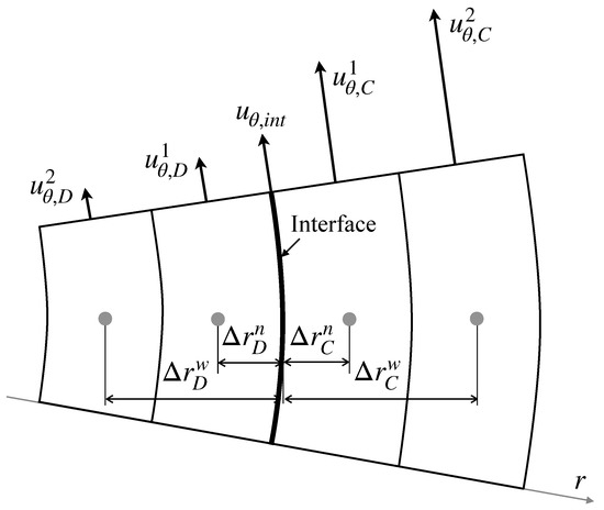
Figure 2. Interface velocity.

Discretization of some derivatives in the governing equations needs a special treatment at the pole ($r=0$). In the evaluation of the divergence of $\mathbf{u}$ and the Laplacian of the velocity components and the pressure, no special treatments are required since the terms $r\varphi$ and $r\partial \varphi /\partial r$ vanish at the pole, where $\varphi =u_r$, $u_{\theta }$ or p. On the other hand, for instance, the finite difference approximation of the advection term $u_r\partial u_{\theta }/\partial r$ requires $u_{\theta }$ at $r=0$. A numerical treatment similar to that in Mohseni and Colonius [30] and Sugioka and Komori [31] is used in this study to set $u_{\theta }$ at $r=0$, i.e., $u_{\theta }(0,\theta )=(u_{\theta }(\Delta r/2,\theta )+u_{\theta }(\Delta r/2,\theta +\pi ))/2$ (Figure 3). Although $0\le \theta \le \pi$, $u_{\theta }(\Delta r/2,\theta +\pi )$ can be set to the value of $u_{\theta }(\Delta r/2,\theta -\pi )$ because of the axial symmetry.

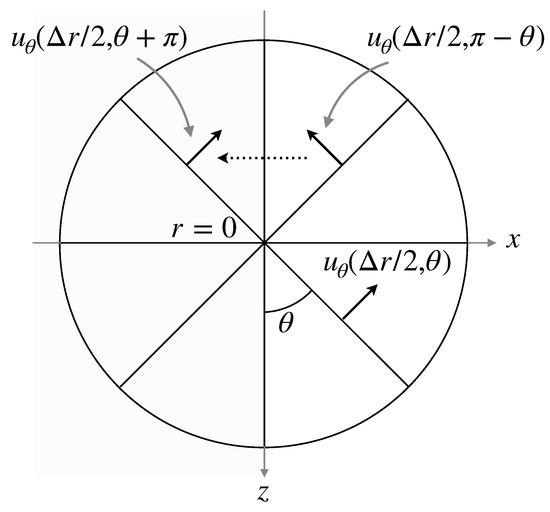
Figure 3. Numerical treatment at pole.

2.2.3. Surfactant Transport Equations

The transport equation of ${\mathsf{\Gamma }}^{\ast }$ is solved using the second-order Runge–Kutta scheme:

$$\begin{array}{cc}\hfill & {\mathsf{\Gamma }}^{\ast \left(1\right)}={\mathsf{\Gamma }}^{\ast n}+\frac{\Delta t^{\ast }}{2}\left[-{\nabla }_S^{\ast }·{\mathbf{u}}_S^{\ast n+1}{\mathsf{\Gamma }}^{\ast n}+\frac{{\nabla }_S^{\ast 2}{\mathsf{\Gamma }}^{\ast n}}{P{e}_S}+{\dot{S}}_{\mathsf{\Gamma }}^{\ast }\left({\mathsf{\Gamma }}^{\ast n}\right)\right]\hfill \end{array}$$

(36)

$$\begin{array}{cc}\hfill & {\mathsf{\Gamma }}^{\ast n+1}={\mathsf{\Gamma }}^{\ast n}+\Delta t^{\ast }\left[-{\nabla }_S^{\ast }·{\mathbf{u}}_S^{\ast n+1}{\mathsf{\Gamma }}^{\ast \left(1\right)}+\frac{{\nabla }_S^{\ast 2}{\mathsf{\Gamma }}^{\ast \left(1\right)}}{P{e}_S}+{\dot{S}}_{\mathsf{\Gamma }}^{\ast }\left({\mathsf{\Gamma }}^{\ast \left(1\right)}\right)\right]\hfill \end{array}$$

(37)

The Runge–Kutta scheme is also used for the transport equation of $C^{\ast }$ as follows:

$$\begin{array}{cc}\hfill & C^{\ast \left(1\right)}=C^{\ast n}+\frac{\Delta t^{\ast }}{2}\left[-{\nabla }^{\ast }·{\mathbf{u}}_D^{\ast n+1}{C}^{\ast n}+\frac{{\nabla }^{\ast 2}{C}^{\ast n}}{P{e}_D}\right]\hfill \end{array}$$

(38)

$$\begin{array}{cc}\hfill & C^{\ast n+1}=C^{\ast n}+\Delta t^{\ast }\left[-{\nabla }^{\ast }·{\mathbf{u}}_D^{\ast n+1}{C}^{\ast \left(1\right)}+\frac{{\nabla }^{\ast 2}{C}^{\ast \left(1\right)}}{P{e}_D}\right]\hfill \end{array}$$

(39)

The advection and diffusion terms are discretized with the second-order ENO and second-order centered difference schemes, respectively.

The bulk concentration, $C_S^{\ast }$, at the interface is evaluated by applying the second-order one-sided finite difference to $\partial C^{\ast }/\partial r^{\ast }$,

$$C_S^{\ast }=\frac{P{e}_{D}K{\dot{S}}_{\mathsf{\Gamma }}^{\ast }+\frac{1}{\Delta r_D^{\ast n}-\Delta r_D^{\ast w}}\left(\frac{\Delta r_D^{\ast w}}{\Delta r_D^{\ast n}}{C}^{\ast 1}-\frac{\Delta r_D^{\ast n}}{\Delta r_D^{\ast w}}{C}^{\ast 2}\right)}{\frac{1}{\Delta r_D^{\ast n}-\Delta r_D^{\ast w}}\left(\frac{\Delta r_D^{\ast w}}{\Delta r_D^{\ast n}}-\frac{\Delta r_D^{\ast n}}{\Delta r_D^{\ast w}}\right)}$$

(40)

and is used to evaluate ${\dot{S}}_{\mathsf{\Gamma }}^{\ast }$. The ${\dot{S}}_{\mathsf{\Gamma }}^{\ast }$ is then used to set the boundary condition, Equation (18). The $u_{\theta ,int}^{\ast }$ is updated for ${\nabla }_S^{\ast }{\sigma }^{\ast }\left({\mathsf{\Gamma }}^{\ast n+1}\right)$.

2.2.4. Solution Procedure

The solution procedure of the numerical method is summarized in the following:

• Set the dimensionless groups (${\rho }_D/{\rho }_C$, $\kappa$, $R{e}_C$, $La$, $P{e}_D$, $P{e}_S$, $Ma$, $\alpha$, K and ${\sigma }_0^{\ast }$); generate computational grids inside and outside the drop; and set the initial conditions for each field variable.
• Evaluate the Marangoni stress, ${\nabla }_S^{\ast }{\sigma }^{\ast }\left({\mathsf{\Gamma }}^{\ast n}\right)$, and set the interface velocity, $u_{\theta ,int}^{\ast n}$, using the boundary condition (Equation (35)).
• Solve Equations (20) and (21) to obtain ${\mathbf{u}}^{†}$.
• Compute the intermediate velocity, ${\mathbf{u}}^{‡}$ using Equations (28) and (29).
• Solve the Poisson equation, Equation (30), to obtain $p^{\ast n+1}$.
• Update the velocity to ${\mathbf{u}}^{\ast n+1}$ using Equations (32) and (33).
• Update the interface velocity, $u_{\theta ,int}^{\ast n+1}$, for ${\mathbf{u}}^{\ast n+1}$.
• Compute the surfactant concentration, $C_S^{\ast n}$, at the interface using Equation (40) with $C^{\ast n}$.
• Solve Equations (36) and (37) to obtain ${\mathsf{\Gamma }}^{\ast n+1}$, where the adsorption–desorption flux, ${\dot{S}}_{\mathsf{\Gamma }}^{\ast }$, is evaluated using Equation (17).
• Set the boundary condition of $C^{\ast }$ at the interface, Equation (18), with ${\dot{S}}_{\mathsf{\Gamma }}^{\ast }$.
• Solve Equations (38) and (39) to obtain $C^{\ast n+1}$.
• Return to Step 2.

3. Validation of Numerical Method

3.1. Clean Drop and Solid Sphere

The numerical method is validated for simple problems with well-accepted correlations, i.e., uniform flows about solid spheres and clean spherical drops. Figure 4 shows the computational domain and the grid system. The dimensionless particle diameter is unity, and the domain size is 40 in the radial direction. The outer boundary of the domain is split into either inflow or outflow. The zero-gradient condition is used for the velocity at the outflow boundary and the outlet pressure is set to zero. The numbers of the computational cells in the r and $\theta$ directions are 25 and 120, respectively. The cell size is uniform in the $\theta$ direction, whereas in the r direction the cell size decreases (increases) toward the drop interface (the outer boundary of the domain) as r increases. For clean drops, it is not necessary to use the very thin computational cells in the vicinity of the drop interface for capturing the velocity boundary layer at low and moderate Reynolds numbers. On the other hand, in the contaminated drop cases discussed in Section 4, the thin cells are required to capture concentration boundary layers of $C^{\ast }$ forming at the interface. Cuenot et al. [10] estimated the dimensionless thickness of the concentration boundary layer as $\delta \sim \sqrt{\pi /\left(4P{e}_C\right)}$ [9] and generated computational grids so as to have at least three computational cells within the boundary layer. The present grid is prepared to meet the same requirement. This grid will also be used in the contaminated drop simulations. The mesh dependence of the predictions was confirmed to be small enough at the present spatial resolution.

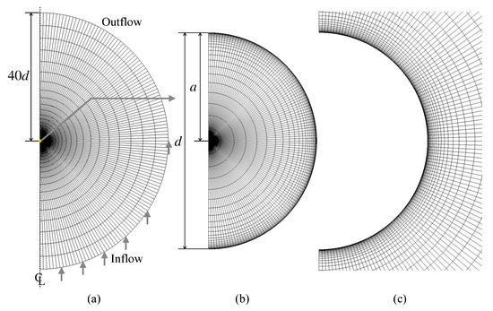
Figure 4. Computational grid. (a) whole domain, (b) drop, (c) continuous phase around drop.

Figure 5 shows predicted $u_{\theta ,int}^{\ast }$ of clean drops at several drop Reynolds numbers, $R{e}_C$, the range of which ($0.1\le R{e}_C\le 20$) covers $R{e}_C$ in the experiment of the contaminated drops [22], i.e., $0.5\le R{e}_C\le 0.73$. The viscosity ratio in the simulations is $\kappa =0.021$. The predicted $u_{\theta ,int}^{\ast }$ at $R{e}_C=0.1$ agrees well with the Hadamard–Rybczynski (HR) solution, $u_{\theta ,int}^{\ast }=sin\theta /\left(2(1+\kappa )\right)$. The slight difference between the prediction and the analytical solution for the Stokes flow is attributed to the presence of a weak inertial effect even at the small Reynolds number. The increase in $R{e}_C$ up to $R{e}_C=1$ makes the inertial effect obvious, i.e., $u_{\theta ,int}$ for $\theta <3\pi /4$ is larger than the HR solution. The deviation from the Stokes flow is increased by further increase in $R{e}_C$.

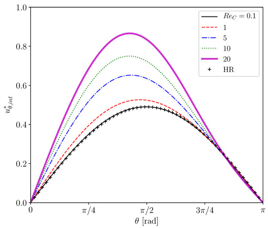
Figure 5. Interface velocities of clean drops at several Reynolds numbers. HR: Hadamard-Rybczynski solution.

Figure 6 shows predicted $C_D$ of clean spherical drops. The open circles are for $\kappa =0.021$ and they are compared with the HR drag (the black dashed line)

$$C_D=\frac{8}{R{e}_C}\left(\frac{2+3\kappa }{1+\kappa }\right)$$

(41)

and the empirical correlation proposed by Myint et al. [32] (the black solid line)

$$C_D=\frac{8}{R{e}_C}\left(\frac{2+3\kappa }{1+\kappa }\right)\left(1+0.15R{e}_C^{0.687}\right)$$

(42)

Figure 6. Drag coefficients, $C_D$, of clean drops and solid spheres. HR: Hadamard–Rybczynski [7,8] (Equation (41)), WM: Win Myint [32] (Equation (42)).

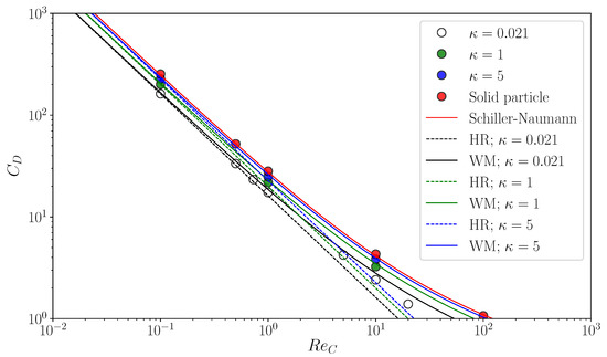
The $C_D$ at $R{e}_C=0.1$ agrees with both drag correlations. The predictions become larger than the HR drag as $R{e}_C$ increases due to the inertial effect. The trend of the drag curve of Equation (42) agrees with that of the data, the values of which are however smaller than those of the correlation since the correlation accounts for the increase in drag by shape deformation. The green and blue symbols in the figure are predictions for $\kappa =1$ and 5, respectively. The simulations reproduce well the increase in $C_D$ by the factor of $(2+3\kappa )/(1+\kappa )$. Simulations of flows about spherical particles are also carried out as the limiting case of $\kappa \to \infty$ by directly applying the no-slip boundary condition to the particle surface. The predicted drag coefficients are shown in the figure by the red symbols and compared with the following empirical correlation proposed by Schiller and Naumann [33]:

$$C_D=\frac{24}{R{e}_C}\left(1+0.15R{e}_C^{0.687}\right)$$

(43)

The data agree well with the correlation. Thus, the present numerical method gives good predictions of the motion of drops for wide ranges of $R{e}_C$ and $\kappa$.

3.2. Contaminated Bubbles

Cuenot et al. [10] carried out numerical simulations of contaminated spherical bubbles in stagnant liquid at $R{e}_C=100$, $P{e}_C=1\times {10}^5$ and $K=1$. They changed $Ma$, $\alpha$ and $La$ to deal with different situations, i.e., the stagnant-cap regime and the fully covered regime. Case 1 ($Ma=61$, $\alpha =0.001$, $La=0.112$), Case 3 ($Ma=61$, $\alpha =0.001$, $La=0.0112$) and Case 4 ($Ma=610$, $\alpha =0.001$, $La=0.112$) in their study are simulated with the present numerical method. The flows inside bubbles are not solved; instead, the tangential viscous stress in the gas phase is set to zero in Equation (6). Figure 7 shows predicted $u_{\theta ,int}^{\ast }$ and ${\mathsf{\Gamma }}^{\ast }$, which are compared with the predictions by Cuenot et al. [10]. The $u_{\theta ,int}^{\ast }$ increases with increasing $\theta$, whereas it steeply decreases to zero at $\theta \sim \pi /4$ and $5\pi /8$ in Cases 1 and 3, respectively. On the other hand, the gradients of ${\mathsf{\Gamma }}^{\ast }$ are large at these $\theta$. The steep decrease in $u_{\theta ,int}^{\ast }$ is due to the Marangoni stress caused by the gradient of ${\mathsf{\Gamma }}^{\ast }$. In comparison with Case 3, ${\mathsf{\Gamma }}^{\ast }$ in the contaminated region is larger in Case 1 and the attenuation of $u_{\theta ,int}^{\ast }$ is more significant because of the larger $La$. In Case 4, $u_{\theta ,int}^{\ast }$ is almost zero, in other words the interface is immobile, due to the large $Ma$, and ${\mathsf{\Gamma }}^{\ast }\approx 0.09$ even at the bubble nose. Thus, being similar to the predictions of Cuenot et al. [10], the effects of $La$ and $Ma$ on $u_{\theta ,int}^{\ast }$ and ${\mathsf{\Gamma }}^{\ast }$ are clearly observed.

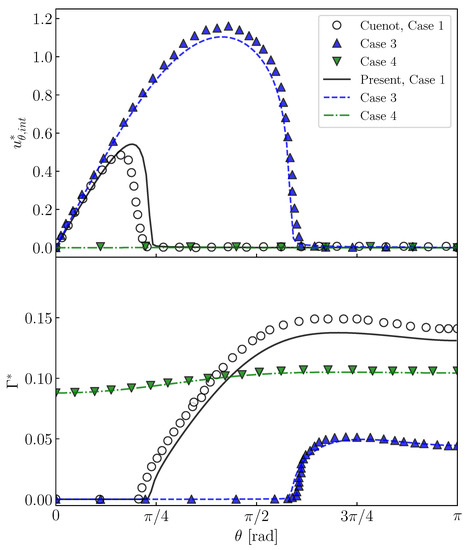
Figure 7. Interface velocities, $u_{\theta ,int}^{\ast }$, and interfacial surfactant concentrations, ${\mathsf{\Gamma }}^{\ast }$ of contaminated bubbles. Steady-state solutions for Cases 1, 3 and 4 in Cuenot et al. [10].

4. Simulations of Contaminated Drops

The main difference in the simulations of contaminated drops carried out in this section is the value of $La$, which ranges from 0 to ${10}^2$, leading to varying surface concentrations. The fluid properties of a drop and a bulk liquid are the same as those in the experiment [22], i.e., those for a glycerol–water solution of 54 wt.% and a silicone oil. They are summarized in Table 1. The drop diameter is $8.3$ mm. Under this condition, $R{e}_C$ is less than unity. Triton X-100 is used for surfactant. The adsorption–desorption properties and the diffusion coefficients of Triton X-100 are shown in Table 2 (see Appendix B for evaluation methods). The $C_0$ in a drop is initially set either to 0 (clean liquid), $0.0020$, $0.0050$, $0.010$ or $0.10$ mol/m${}^3$. These conditions are referred to as Cases 1, 2, 3, 4 and 5, respectively. The concentrations are less than the critical micellar concentration (0.28 mol/m${}^3$). The measurements were carried out at 250 mm below the nozzle tip. The dimensionless time when drops reached the measurement region was 30. The relevant dimensionless groups in each case are summarized in Table 3. These values of the dimensionless groups are used as the input parameters of the numerical simulations. See Hosokawa et al. [22] for further details of the experimental conditions.

Table 1. Fluid properties of glycerol–water solution of 54 wt.% and silicone oil at 298 K [22].

Phase	Dispersed	Continuous
$\rho$ [kg/m${}^3$]	1132	967
$\mu$ [Pa·s]	0.00613	0.299
${\sigma }_0$ [N/m]	0.0343

Table 2. Properties of Triton X-100 [22].

${\mathit{k}}_{\mathit{a}}$ [m${}^3$/mol·s]	${\mathit{k}}_{\mathit{d}}$ [1/s]	${\mathbf{\Gamma }}_{\mathbf{max}}$ [mol/m${}^2$]	${\mathit{D}}_{\mathit{D}}$ [m${}^2$/s]	${\mathit{D}}_{\mathit{S}}$ [m${}^2$/s]
9.4	0.0096	1.69 × 10${}^{-6}$	2 × 10${}^{-10}$	2 × 10${}^{-10}$

Table 3. Dimensionless groups.

Case	1	2	3	4	5
${\mathit{C}}_0$ [mol/m${}^3$]	0	0.0020	0.0050	0.010	0.10
${\rho }_D/{\rho }_C$	1.17	1.17	1.17	1.17	1.17
$\kappa$	0.021	0.021	0.021	0.021	0.021
$R{e}_D$	42	39	34	30	29
$R{e}_C$	0.73	0.68	0.59	0.52	0.50
$La$	0	2.0	4.9	9.8	98
$P{e}_D\times {10}^{-6}$	-	1.1	0.91	0.80	0.77
$P{e}_S\times {10}^{-6}$	-	1.1	0.91	0.80	0.77
$Ma$	-	0.55	0.64	0.72	0.75
$\alpha$	-	0.0062	0.018	0.040	0.42
K	-	0.10	0.041	0.020	0.0020
${\sigma }_0^{\ast }$	8.2	8.2	8.2	8.2	8.2

Figure 8a shows flow fields in Case 1 ($C_0=0$ mol/m${}^3$). The left half is the flow field visualized by integrating the grayscale values in high-speed video images while tracking the drop; the flow structure is therefore observed from the frame of reference moving with the drop. The liquid in the outside of the drop flows from the nose ($\theta =0$) side to the rear ($\theta =\pi$) side and no separation of the flow takes place. Inside the drop, an internal circulation is formed. Hence the interface is mobile. The right half of the figure shows the predicted velocity vectors inside and outside the drop. The number of the velocity vectors are reduced for visualization purposes. The flow characteristics inside and outside the drop agree with the measurement.

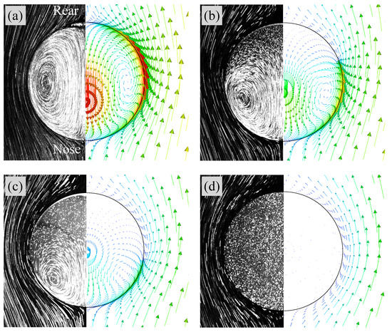
Figure 8. Comparisons of flow fields between predictions and experimental data [22]. (a) Case 1 (clean), (b) Case 3, (c) Case 4, (d) Case 5. Right: predicted; Left: measured (Reprinted from International Journal of Multiphase Flow 97, S. Hosokawa, Y. Masukura, K. Hayashi, A. Tomiyama, Experimental evaluation of Marangoni stress and surfactant concentration at interface of contaminated single spherical drop using spatiotemporal filter velocimetry, 157–167, Copyright (2017), with permission from Elsevier).

Figure 9 shows ${\mathsf{\Gamma }}^{\ast }$ at $t^{\ast }=10,20$ and 30. In Case 2 ($C_0=0.0020$ mol/m${}^3$), ${\mathsf{\Gamma }}^{\ast }$ increases in the rear region of the drop as $t^{\ast }$ increases. The contaminated area also increases, but is not so large even at $t^{\ast }=30$. In Case 3 ($C_0=0.0050$ mol/m${}^3$) and 4 ($C_0=0.010$ mol/m${}^3$), the trend of the temporal change in ${\mathsf{\Gamma }}^{\ast }$ is similar to that in Case 1, whereas the contaminated area becomes much wider as $C_0$ increases. The ${\mathsf{\Gamma }}^{\ast }$ in Case 5 ($C_0=0.10$ mol/m${}^3$) is much larger than the other cases, and the whole interface is contaminated. The presence of surfactant reduces the region of the internal circulation both in the experiment and simulation of Case 3 as shown in Figure 8b (the flow field of Case 2, whose flow characteristics are in-between those of Cases 1 and 3, was omitted for saving the space). The magnitude of the drop velocity in the vicinity of the drop rear is very small. The increase in $C_0$ from $0.0050$ mol/m${}^3$ to $0.010$ mol/m${}^3$ (Case 4) makes the circulation region smaller (Figure 8c). The interface velocity in the rear half, $\theta >\pi /2$, is close to zero, so that the formation of velocity boundary layer along the interface can be clearly observed in the continuous phase. In Case 5 (Figure 8d), no internal circulation is formed inside the drop. In the continuous phase, the grayscale values near the interface in the measurement are very low (almost black), which implies that the velocities there are very small. The prediction agrees with the measurement; the interface velocity is almost zero at the whole interface; in other words, the interface is fully contaminated and immobile, so that the velocity field outside the drop seems to be similar to that about a solid sphere.

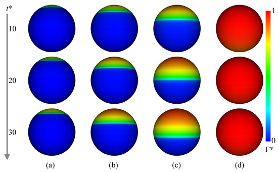
Figure 9. Time evolutions of ${\mathsf{\Gamma }}^{\ast }$. (a) Case 2; (b) Case 3; (c) Case 4; (d) Case 5.

Figure 10a shows the distribution of $C^{\ast }$ in Case 2. The $t^{\ast }$ increases from the left to the right. The rightmost figures are magnified views of the regions labeled by (i) and (ii). The $C^{\ast }$ near the interface in the rear region decreases at $t^{\ast }=5$. The low $C^{\ast }$ region develops toward the centerline of the drop as $t^{\ast }$ increases due to the advection. However $C^{\ast }$ near the rear does not decrease so much. Because of the low diffusion coefficient, the pattern of the low $C^{\ast }$ region is determined by the advection and does not smear out. Figure 11 shows the time evolution of $C_S^{\ast }$ in Case 2. The surfactant flux from the bulk to the interface decreases $C^{\ast }$ in the vicinity of the interface and the weak diffusion cannot compensate for the reduction in $C^{\ast }$ by adsorption. The $C_S^{\ast }$ at $t^{\ast }=5$ is therefore smaller than the initial value, $C_S^{\ast }=1$. The $\theta$ for the minimum $C_S^{\ast }$ corresponds to that for steep velocity decrease; in other words, the stagnant-cap angle, ${\theta }_{cap}$. For $\theta <{\theta }_{cap}$, ${\mathsf{\Gamma }}^{\ast }$ is very small, so that the adsorption is dominant in the surfactant flux. The increase in $C_S^{\ast }$ with increasing $\theta$ for $\theta >{\theta }_{cap}$ implies that the desorption increases $C_S^{\ast }$ in the stagnant-cap region. In the stagnant-cap region, ${\mathsf{\Gamma }}^{\ast }$ approaches a value for the local adsorption–desorption equilibrium, ${\mathsf{\Gamma }}^{\ast }\sim 1/(1+{\left(C_S^{\ast }\right)}^{-1})$. The $u_{\theta ,int}^{\ast }$ is very small in that region, but is still non-zero. The weak interface compression effect ($\mathsf{\Gamma }{\nabla }_S·{\mathbf{u}}_S$) appears and slightly increases ${\mathsf{\Gamma }}^{\ast }$. However, some excess amount of surfactant is desorbed from the interface to the bulk. Thus, $C_S^{\ast }$ has an increasing trend in the high $\theta$ region. At larger $t^{\ast }$, $C_S^{\ast }$ decreases moderately for $\theta <{\theta }_{cap}$, whereas for $\theta >{\theta }_{cap}$$C_S^{\ast }$ increases and becomes larger than unity.

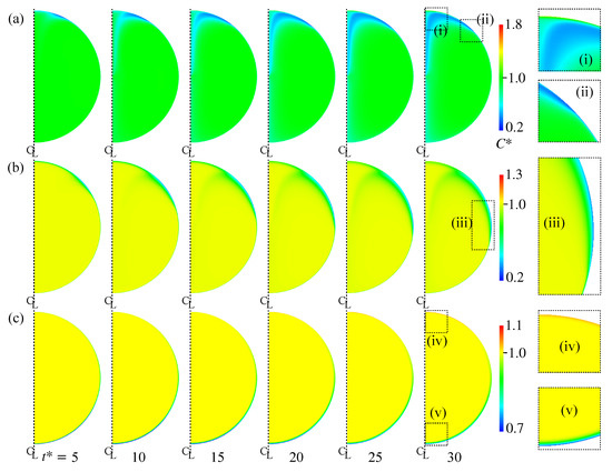
Figure 10. Time evolutions of $C^{\ast }$. (a) Case 2; (b) Case 4; (c) Case 5. The time $t^{\ast }$ increases from left to right, whereas the rightmost figures are magnified views of the distribution at $t^{\ast }=30$.

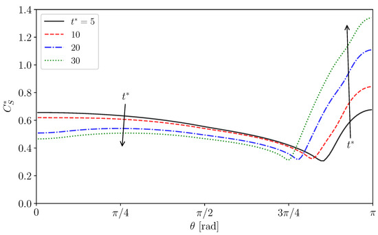
Figure 11. Surfactant concentration, $C_S^{\ast }$, at interface in Case 2.

Figure 10b shows the time evolution of $C^{\ast }$ in Case 4. As shown in the magnified view of $C^{\ast }$ near the interface (iii), a low $C^{\ast }$ region is formed around the drop equator. The interface area is more than half covered with surfactant at this moment (Figure 9c). The formation of the low $C^{\ast }$ region is therefore the result of surfactant adsorption from the bulk to the interface. The thickness of the concentration boundary layer is, as expected, very thin because of the high $P{e}_D$. In Case 5, the whole interface is covered by surfactant as shown in Figure 9d, which results in the formation of the thin concentration boundary layer of low $C^{\ast }$ in the nose region (Figure 10c(v)). As it is similar to Case 2, the interface compression effect increases ${\mathsf{\Gamma }}^{\ast }$ in the rear half of the drop and the desorption becomes dominant near the rear, resulting in the formation of boundary layer of $C^{\ast }$ larger than unity in the rear region (the magnified view (iv)).

Figure 12 shows the pressure distribution in Case 3, in which $p_D^{\ast }$ and $p_C^{\ast }$ are subtracted by the pressure, $p_0^{\ast }$, at the drop center and the far field pressure, $p_{\infty }^{\ast }=0$, respectively. The ${\theta }_{cap}$ represents the cap angle evaluated from the velocity distribution and ${\theta }_{cap}\sim 0.6\pi$ rad. In the pressure distribution, high-pressure spots are formed in the vicinity of the interface at $\theta$ slightly smaller than ${\theta }_{cap}$. Comparing $p^{\ast }$ with the velocity field clearly shows that these high-pressure spots prevent the fluid motion along the interface, which results in the formation of the stagnant-cap region in the rear half of the drop and the attenuation of the tangential velocity in the continuous phase.

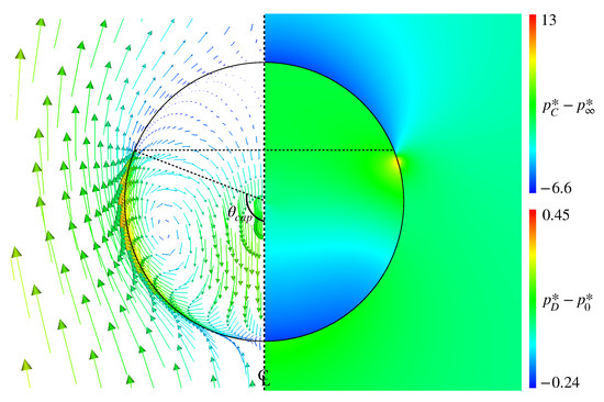
Figure 12. Pressure distributions inside and outside drop in Case 3 (right). The velocity field is also shown for comparing the high-pressure location with the cap angle, ${\theta }_{cap}\sim 0.6\pi$ rad (left).

Figure 13a shows the interface velocity, $u_{\theta ,int}^{\ast }$, at $t^{\ast }=30$. The lines and symbols are the predictions and the measured data [22], respectively. The predicted velocity of the clean drop (Case 1) agrees fairly with the data, except for the rear region. The lower values at large $\theta$ in the data are due to slight contamination in the rear region, the cause of which would be contamination brought into the drop by seeding particles. The retardation effect of surfactant in $u_{\theta ,int}^{\ast }$ is clearly seen in both data and predictions of Cases 2–5. In Case 2, the predicted velocity profile agrees with the data. The $u_{\theta ,int}^{\ast }$ decreases from $\theta \sim \pi /2$ as $\theta$ increases and becomes very small for $\theta >3\pi /4$, i.e., ${\theta }_{cap}\sim 3\pi /4$. The increase in $C_0$ decreases ${\theta }_{cap}$, i.e., ${\theta }_{cap}$ are $0.6\pi$ and $0.45\pi$ rad in Case 3 and 4, respectively. Although the predicted velocities are somewhat larger than the data, the dependence of $u_{\theta ,int}^{\ast }$ on $C_0$ is reproduced. In Case 5, $u_{\theta ,int}^{\ast }\sim 0$ at any $\theta$ as already seen in Figure 8.

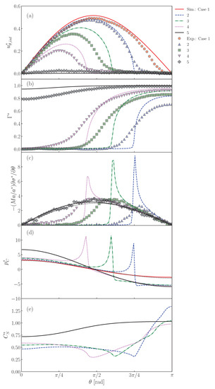
Figure 13. Predictions of (a) $u_{\theta ,int}^{\ast }$, (b) ${\mathsf{\Gamma }}^{\ast }$, (c) $-Ma\partial {\sigma }^{\ast }/\partial \left(a^{\ast }\theta \right)$, (d) $p_C^{\ast }$ and (e) $C_S^{\ast }$ at interface. The symbols and lines are measured [22] and predicted values, respectively. The black dotted line in $\partial {\sigma }^{\ast }/\partial \left(a^{\ast }\theta \right)$ represents the dimensionless velocity gradient, ${\left.\partial u_{\theta }^{\ast }/\partial r^{\ast }\right|}_{r^{\ast }=a^{\ast }}=3sin\theta$, given by the Stokes solution for solid sphere. The black dotted line in $p_C^{\ast }$ is also the Stokes solution given by $p_C^{\ast }=3cos\theta /\left(2R{e}_C\right)$.

The distributions of ${\mathsf{\Gamma }}^{\ast }$ are shown in Figure 13b. The predicted ${\mathsf{\Gamma }}^{\ast }$ of Case 2 is almost zero for $\theta <{\theta }_{cap}$, whereas it steeply increases and reaches a large value for $\theta >{\theta }_{cap}$, which is larger than $La/(1+La)=0.67$ for the absorption-desorption equilibrium for $C_0$ since $C_S^{\ast }$ in this region is larger than unity (Figure 11). The measured ${\mathsf{\Gamma }}^{\ast }$ shows a similar profile, while the following differences are present: the measured ${\mathsf{\Gamma }}^{\ast }$ is smoother around $\theta ={\theta }_{cap}$ than predicted and approaches $0.67$. The increase in $C_0$ (Cases 3 and 4) increases ${\mathsf{\Gamma }}^{\ast }$, whereas the drop nose is still almost clean. On the other hand, ${\mathsf{\Gamma }}^{\ast }$ takes a large value even at the nose in Case 5 since the adsorption is much more dominant than the desorption as represented by the large $La$.

As shown in Figure 13c, peaks appear in the predicted Marangoni stresses in Cases 2, 3 and 4. However, in Case 5, there are no peaks. This is due to the smaller ${\mathsf{\Gamma }}^{\ast }$ gradient. Despite a smaller ${\mathsf{\Gamma }}^{\ast }$ gradient, the Marangoni stress immobilizes the interface almost completely since the Marangoni stress acts on the whole interface. In this situation, the Marangoni stress agrees very well with the viscous stress acting on the solid sphere given by the Stokes solution (the black dotted line in the figure), i.e., ${\left.\partial u_{\theta }^{\ast }/\partial r^{\ast }\right|}_{r^{\ast }=a^{\ast }}=3sin\theta$. The smaller peaks in the data are attributed to a smoother distribution of ${\mathsf{\Gamma }}^{\ast }$.

The peaked distribution of the Marangoni stress also causes similar peaks in the pressure distribution as shown in Figure 13d. The locations of the strong Marangoni stress correspond to those of the steep velocity reduction (the cap angles). The peaks of the pressure however locate at slightly smaller $\theta$. This trend was already observed in Figure 12. The pressure distribution in Case 5 is smooth as in the clean drop case and agrees well with the Stokes solution given by $p_C^{\ast }=3cos\theta /\left(2R{e}_C\right)$.

In the distributions of $C_S^{\ast }$ shown in Figure 13d, $\theta$ for the minimum $C_S^{\ast }$ in Cases 2–4 roughly correspond to ${\theta }_{cap}$. The $C_S^{\ast }$ in these cases exhibit the increasing trend in the stagnant-cap region. On the other hand, on the completely immobilized interface in Case 5, the profile of $C_S^{\ast }$ monotonically increases with increasing $\theta$.

The measured ${\mathsf{\Gamma }}^{\ast }$ is much smoother than predicted, which suggests that in reality $P{e}_S$ is much lower than that used in the simulation or that there is some other transport process much more effective for interface transport. A brief discussion on this point is given in Appendix C.

5. Conclusions

The motion of contaminated spherical drops falling through a stagnant liquid were numerically simulated using the finite difference method to investigate the effects of surfactant on the flow inside and outside the drops. The numerical method was first validated through simulations of spherical particles, clean drops and contaminated bubbles. The predicted drag coefficients of the spherical particles and clean drops agreed well with available drag correlations. The interface velocity and the interfacial surfactant concentration of contaminated bubbles also agreed with those predicted in the literature [10]. The numerical simulations of contaminated drops were then carried out. The numerical conditions were the same as those in the experiment carried out in Hosokawa et al. [22], i.e., the fluid properties for the drop and the bulk liquid were for a glycerol–water solution and a silicone oil, respectively, and the surfactant was Triton X-100. The drop Reynolds numbers were less than unity and the drop shape kept spherical. The surfactant concentration, $C_0$, was varied below the critical micellar concentration; $C_0=0.0020$, $0.0050$, $0.010$ and $0.10$ mol/m${}^3$ in Cases 1, 2, 3, 4 and 5, respectively. The characteristics of the field variables can be summarized as follows:

• The predicted interfacial surfactant concentration, $\mathsf{\Gamma }$, is almost zero for the angle, $\theta$, smaller than a certain value (${\theta }_{cap}$), whereas it steeply increases and reaches a large value for $\theta >{\theta }_{cap}$. The interface velocity, $u_{\theta ,int}$, decreases as $\theta$ increases and becomes very small for $\theta >{\theta }_{cap}$. The increase in $C_0$ increases $\mathsf{\Gamma }$ and decreases ${\theta }_{cap}$. The presence of surfactant attenuates the internal circulation and the increase in $C_0$ makes the circulation region smaller.
• The surfactant flux from the bulk to the interface decreases C in the vicinity of the interface and the weak diffusion cannot compensate for the reduction in C by adsorption. The bulk concentration, $C_S$, at the interface therefore tends to be smaller than $C_0$ for $\theta <{\theta }_{cap}$. The pattern of the low C region is determined by the advection and does not smear out because of a small diffusive flux.
• Peaks appear in the predicted Marangoni stresses in Cases 2–4, while in Case 5 no peaks develop due to a smaller $\mathsf{\Gamma }$ gradient. The peaked distribution of the Marangoni stress also causes similar peaks in the pressure distribution. The locations of the strong Marangoni stress correspond to ${\theta }_{cap}$, whereas the peaks of the pressure appear at slightly smaller $\theta$. The high-pressure spots prevent the fluid motion along the interface, which results in the formation of the stagnant-cap region in the rear half of the drop and the attenuation of the tangential velocity in the continuous phase.

References

- Clift, R.; Grace, J.R.; Weber, M.E. Bubbles, Drops, and Particles; Academic Press: New York, NY, USA, 1978. [Google Scholar]
- Takagi, S.; Uda, T.; Watanabe, Y.; Matsumoto, Y. Behavior of a rising bubble in water with surfactant dissolution (1st report, steady behavior). Trans. JSME 2003, 69, 2192–2199. (In Japanese) [Google Scholar] [CrossRef][Green Version]
- Landau, L.D.; Lifshitz, E.M. Fluid Mechanics, 2nd ed.; Butterworth-Heinemann: Oxford, UK, 1987. [Google Scholar]
- Aoki, J.; Hayashi, K.; Hosokawa, S.; Tomiyama, A. Effects of surfactant on mass transfer from single carbon dioxide bubbles in vertical pipes. Chem. Eng. Technol. 2015, 38, 1955–1964. [Google Scholar] [CrossRef]
- Boussinesq, J. Vitesse de la chute lente, devenue uniforme, d’une goutte liquide spherique. dans un fluid visqueux de poids specifique moindre. C. R. Acad. Sci. 1913, 156, 1124–1130. [Google Scholar]
- Scriven, L.E. Dynamics of a fluid interface. Chem. Eng. Sci. 1960, 12, 98–108. [Google Scholar] [CrossRef]
- Hadamard, J.S. Mouvement permanent tent d’une sphere liquide et visquese dans un liquide visqueux. Comptes Rendus I’Acad. Des Sci. 1911, 152, 1735–1738. [Google Scholar]
- Rybczynski, W. On the translatory of a fluid sphere in a viscous medium. Bull. Acad. Sci. Kracow Ser. 1911, 3, 40–46. [Google Scholar]
- Levich, V.G. Physicochemical Hydrodynamics; Prentice Hall: Englewood Cliffs, NJ, USA, 1962. [Google Scholar]
- Cuenot, B.; Magnaudet, J.; Spennato, B. The effects of slightly soluble surfactants on the flow around a spherical bubble. J. Fluid Mech. 1997, 339, 25–53. [Google Scholar] [CrossRef]
- Takagi, S.; Ogasawara, T.; Fukuta, M.; Matsumoto, Y. Surfactant effect on the bubble motions and bubbly flow structures in a vertical channel. Fluid Dyn. Res. 2009, 41, 065003. [Google Scholar] [CrossRef]
- Muradoglu, M.; Tryggvason, G. A front-tracking method for computation of interfacial flows with soluble surfactants. J. Comput. Phys. 2008, 227, 2238–2262. [Google Scholar] [CrossRef]
- Hayashi, K.; Tomiyama, A. Effects of surfactant on terminal velocity of a Taylor bubble in a vertical pipe. Int. J. Multiph. Flow 2012, 39, 78–87. [Google Scholar] [CrossRef]
- Hayashi, K.; Tomiyama, A. Effects of numerical treatment of viscous and surface tension forces. J. Comput. Multiph. Flows 2014, 6, 111–126. [Google Scholar] [CrossRef]
- Engberg, R.F.; Wegener, M.; Kenig, E.Y. The influence of Marangoni convection on fluid dynamics of oscillating single rising droplets. Chem. Eng. Sci. 2014, 117, 114–124. [Google Scholar] [CrossRef]
- Atasi, O.; Haut, B.; Pedrono, A.; Scheid, B.; Legendre, D. Influence of soluble surfactants and deformation on the dynamics of centered bubbles in cylindrical microchannels. Langmuir 2018, 34, 10048–10062. [Google Scholar] [CrossRef] [PubMed]
- Shin, S.; Chergui, J.; Juric, D.; Kahouadji, L.; Matar, O.; Craster, R. A hybrid interface tracking-level set technique for multiphase flow with soluble surfactant. J. Comput. Phys. 2018, 359, 409–435. [Google Scholar] [CrossRef]
- Piedfert, A.; Lalanne, B.; Masbernat, O.; Risso, F. Numerical simulations of a rising drop with shape oscillations in the presence of surfactants. Phys. Rev. Fluids 2018, 3, 103605. [Google Scholar] [CrossRef]
- Batchvarov, A.; Kahouadji, L.; Magnini, M.; Constante-Amores, C.; Shin, S.; Chergui, J.; Juric, D.; Craster, R.; Matar, O. Effect of surfactant on elongated bubbles in capillary tubes at high Reynolds number. Phys. Rev. Fluids 2020, 5, 093605. [Google Scholar] [CrossRef]
- Ubal, S.; Brown, N.; Lu, J.; Corvalan, C. Active motion of contaminated microbubbles. Chem. Eng. Sci. 2021, 238, 116574. [Google Scholar] [CrossRef]
- Dukhin, S.S.; Kretzschmar, G.; Miller, R. Dynamics of Adsorption at Liquid Interfaces; Elsevier Science: Amsterdam, The Netherlands, 1995. [Google Scholar]
- Hosokawa, S.; Masukura, Y.; Hayashi, K.; Tomiyama, A. Experimental evaluation of Marangoni stress and surfactant concentration at interface of contaminated single spherical drop using spatiotemporal filter velocimetry. Int. J. Multiph. Flow 2017, 97, 157–167. [Google Scholar] [CrossRef]
- Hosokawa, S.; Tomiyama, A. Spatial Filter Velocimetry based on Time-Series Particle Images. Exp. Fluids 2012, 52, 1361–1372. [Google Scholar] [CrossRef]
- Batchelor, G.K. An Introduction to Fluid Dynamics; Cambridge University Press: Cambridge, UK, 1967. [Google Scholar]
- Stone, H.A. A simple derivation of the time-dependent convective-diffusion equation for surfactant transport along a deforming interface. Phys. Fluids 1990, 2, 111–112. [Google Scholar] [CrossRef]
- Frumkin, A.; Levich, V.G. On surfactants and interfacial motion. Zhurnal Fiz. Khimii 1947, 21, 1183–1204. (In Russian) [Google Scholar]
- Kim, J.; Moin, P. Application of a Fractional-Step Method to Incompressible Navier-Stokes Equations. J. Comput. Phys. 1985, 323, 308–323. [Google Scholar] [CrossRef]
- Choi, H.; Moin, P. Effects of the computational time step on numerical solutions of turbulent flow. J. Comput. Phys. 1994, 113, 1–4. [Google Scholar] [CrossRef]
- Shu, C.; Osher, S. Efficient implementation of essentially non-oscillatory shock-capturing schemes. J. Comput. Phys. 1988, 77, 439–471. [Google Scholar] [CrossRef]
- Mohseni, K.; Colonius, T. Numerical treatment of polar coordinate singularities. J. Comput. Phys. 2000, 157, 787–795. [Google Scholar] [CrossRef]
- Sugioka, K.; Komori, S. Drag and lift forces acting on a spherical water droplet in homogeneous linear shear air flow. J. Fluid Mech. 2007, 570, 155–175. [Google Scholar] [CrossRef]
- Myint, W.; Hosokawa, S.; Tomiyama, A. Terminal velocity of single drops in stagnant liquids. J. Fluid Sci. Technol. 2006, 1, 72–81. [Google Scholar] [CrossRef]
- Schiller, L.; Naumann, A. Über die grundlegende Berechnungen bei der Schwerkraft-aufbereitung. Z. Des Vereines Dtsch. Ingenieure 1933, 77, 318–320. [Google Scholar]
- Ward, A.F.H.; Tordai, L. Time-dependence of Boundary Tensions of Solutions: I. the role of diffusion in time-effects. J. Chem. Phys. 1946, 14, 453–461. [Google Scholar] [CrossRef]
- Valkovska, D.S.; Danov, K.D. Determination of Bulk and Surface Diffusion Coefficients from Experimental Data for Thin Liquid Film Drainage. J. Colloid Interface Sci. 2000, 223, 314–316. [Google Scholar] [CrossRef]
- Morgan, C.E.; Breward, C.J.W.; Griffiths, I.M.; Howell, P.D.; Penfold, J.; Thomas, R.K.; Tucker, I.; Petkov, J.T.; Webster, J.R.P. Kinetics of Surfactant Desorption at an Air-Solution Interface. J. Colloid Interface Sci. 2012, 28, 17339–17348. [Google Scholar] [CrossRef] [PubMed]
Publisher’s Note: MDPI stays neutral with regard to jurisdictional claims in published maps and institutional affiliations. |
© 2022 by the authors. Licensee MDPI, Basel, Switzerland. This article is an open access article distributed under the terms and conditions of the Creative Commons Attribution (CC BY) license (https://creativecommons.org/licenses/by/4.0/).