Magnetohydrodynamic Flow of a Bingham Fluid in a Vertical Channel: Mixed Convection

Abstract

In this paper, we describe our study of the mixed convection of a Boussinesquian Bingham fluid in a vertical channel in the absence and presence of an external uniform magnetic field normal to the walls. The velocity, the induced magnetic field, and the temperature are analytically obtained. A detailed analysis is conducted to determine the plug regions in relation to the values of the Bingham number, the buoyancy parameter, and the Hartmann number. In particular, the velocity decreases as the Bingham number increases. Detailed considerations are drawn for the occurrence of the reverse flow phenomenon. Moreover, a selected set of diagrams illustrating the influence of various parameters involved in the problem is presented and discussed.

1. Introduction

In recent years, magnetohydrodynamics has been the subject of many papers because of its relevant industrial applications. The elements of many magnetohydrodynamic devices are made in the form of long channels filled by rheological fluids. In this paper, we detail our study of the steady flow in the absence or in the presence of a uniform external magnetic field of an electrically conducting Bingham fluid in a vertical channel whose walls are heated at constant different temperatures. We analyze the mixed convection by continuing our previous study [1] in which we treated the natural convection.

Bingham fluids are non-Newtonian viscoplastic fluids that possess a yield stress below which they behave as rigid solids and as viscous fluids if the shear stress exceeds the yield stress. Therefore, they appear in the channel plug regions, which are a priori unknown and have to be determined as part of the solution of the problem.

We recall that Bingham fluid is one of the simplest models of a viscoplastic fluid [2]. This kind of fluid modelizes many materials as, for example, muds used in oil extractive industry, cements, ceramics, molten plastics in extrusion processes, and also biological fluids in particular conditions.

Many papers are devoted to the study of Bingham fluids both from a theoretical and a practical point of view. Existence of weak solutions for the system governing the motion is investigated in [3], studies nonlinear stability of Poiseuille flow in pipes and plane channels in [4], spatial decay estimates are obtained for the problem of entry flow in a pipe in [5], and Couette–Poiseuille flow in a porous channel is studied with slip conditions in [6]. Some papers deal with the convective flow of a Bingham fluid in a vertical channel: the natural convection is studied in [7] for the Couette–Poiseuille flow and in [8,9] for the Poiseuille flow, the effect of internal and external heating on the free convective flow in a porous channel is investigated using Pascal’s piecewise-linear law in [10], and the mixed convection is analyzed in [11].

In this research, the flow in the channel is steady and fully-developed, and the walls are vertical and kept at uniform different temperatures. We suppose that the external body forces are due to the gravity and the fluid is slightly compressible so that the Oberbeck–Boussinesq approximation is adopted. Moreover, a constant vertical pressure gradient is applied in order to have mixed convection.

This topic has been studied extensively for Newtonian fluids. A relevant characteristic is that asymmetric wall temperatures produce a skewness in the velocity profile and, if the buoyancy parameter is large enough, the reverse flow can occur near the walls ([12,13,14,15]). As far as Bingham fluids are concerned, the unique study is due to Patel and Ingham ([11]), who outline that three different profiles of the velocity are possible if one assumes that the magnitude of the stress at the hot wall is greater than the yield stress.

In this paper, we complete the analysis developed in [11]. Actually, many considerations in [11] are only sketched and the limitations to which the Bingham number B and the buoyancy parameter $\lambda$ must satisfy in order to have plug regions are not obtained. In the second part of our study, we suppose the presence of an external uniform magnetic field orthogonal to the heated walls. Such a magnetic field generates the Lorentz forces that influence the motion as in the well-known Hartmann flow. We notice that literature in this area of research is poor ([1,16,17,18]), and in most cases, the induced magnetic field is not taken into account.

As previously mentioned, our paper is divided in two parts. The first one (Section 2 and Section 3) is devoted to study the mixed convection in the absence of the external magnetic field in detail. We find that the stress depends on an integration constant $C_0$ that is a priori unknown. Unlike the natural convection in which the problem is symmetric ([1]), in the mixed convection, we have to distinguish three cases depending on the value of the stress on the coldest wall. We find the analytical expressions of the velocity in the three cases mentioned above and the plug regions are determined together with the value of the constant $C_0$. In order to determine the value of $C_0$, we match the expressions of the velocity at the interfaces between plug regions and no plug regions. The plug regions depend on the Bingham number B and on the buoyancy parameter $\lambda$. We obtain that the first case is possible only if $B<1$ without a priori restrictions on $\lambda$, whereas the other two cases are possible only if $\lambda >2$ while B may assume also values $\ge 1$. In Section 3.1, the velocity behavior is analyzed and the plug regions are described. In particular, the velocity decreases as B increases and the maximum of the velocity increases as $\lambda$ increases. In the third case, the reverse flow phenomenon ([7,14,15]) can occur near the cold wall. This situation happens when the magnitude of the buoyancy parameter is large enough.

The latter part concerns the flow in the presence of external the magnetic field (Section 4). We point out that we do not neglect the induced magnetic field because we do not impose restrictions on the magnetic Reynolds number. For this reason, it is much more complex to treat the problem because there is another unknown field: the induced magnetic field. In this situation, the significant component of the deviatoric part of the stress tensor depends on the induced magnetic field, which is unknown, and so we cannot obtain the plug regions in terms of the material parameters alone as we did in Section 3. We find that the presence of the external magnetic field tends to prevent the reverse flow as for a Newtonian fluid. The influence of B and $\lambda$ on the velocity is analogous to that of Section 3. As the Hartmann number M increases, the velocity decreases and the plug region increases its thickness with M. As far as the induced magnetic field h is concerned, the trend is similar to the Newtonian case ([14]). In particular, h is a decreasing function of B and is a increasing function of $\lambda$, whereas the modulus of the induced magnetic field is not monotone when M changes. In Section 6, we summarize the principal results obtained.

2. The Problem and the Governing Equations

In this section and in the next, we complete the study of the problem considered in [11] on the fully developed steady flow of a homogeneous Bingham fluid. Actually, many details in [11] are only sketched and the constraints that must be fulfilled by the Bingham number B and by the buoyancy parameter $\lambda$ in order to have plug regions are not given. Moreover, we study in the details the influence of B and $\lambda$ on the velocity profile and on the thickness of the plug regions.

Let us suppose that the motion occurs in the region $\mathcal{S}$ between two infinite rigid, fixed, and vertical plates ${\mathrm{\Pi }}_1,{\mathrm{\Pi }}_2$ separated by a distance $2d$ (Figure 1).

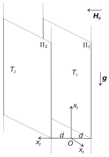
Figure 1. Physical configuration and coordinate system ($T_2>T_1)$.

We assume that

$$\begin{array}{cc}\hfill & \mathcal{S}=\{(x_1,x_2,x_3)\in {\mathbb{R}}^3:(x_1,x_3)\in {\mathbb{R}}^2,x_2\in (-d,d)\},\hfill \\ \hfill & {\mathrm{\Pi }}_i=\{(x_1,x_2,x_3)\in {\mathbb{R}}^3:(x_1,x_3)\in {\mathbb{R}}^2,x_2={(-1)}^{i}d\},i=1,2\hfill \end{array}$$

and $x_1$-axis is vertical upward.

The fluid is heat-conducting and the walls ${\mathrm{\Pi }}_{1,2}$ are kept at uniform temperature $T_{1,2}$ with $T_1<T_2$. Moreover, the fluid is assumed slightly compressible so that, under the Oberbeck–Boussinesq approximation, the governing equations can be written as follows

$$\begin{array}{c}{\rho }_0\mathbf{v}·\nabla \mathbf{v}=-\nabla p+\nabla ·{\mathbf{T}}^D+{\rho }_0[1-\alpha (T-T_0)]\mathbf{g},\hfill \end{array}$$

(1a)

$$\begin{array}{c}\nabla ·\mathbf{v}=0,\hfill \end{array}$$

(1b)

$$\begin{array}{c}\nabla T·\mathbf{v}=b\Delta T\hfill \end{array}$$

(1c)

where $\mathbf{v}$ is the velocity, p is the pressure, ${\mathbf{T}}^{\mathbf{D}}$ is the deviatoric part of the stress tensor $\mathbf{T}$, ${\rho }_0$ is the constant mass density at the reference temperature ${\displaystyle T_0=\frac{T_1+T_2}{2}}$, $\alpha$ is the thermal expansion coefficient, T is the (absolute) temperature, $\mathbf{g}=-g{\mathbf{e}}_1$ is the gravity acceleration, and b is the thermal diffusivity.

In the energy Equation (1a), we have neglected the dissipative terms, as is usual in the Oberbeck–Boussinesq approximation.

As known, the deviatoric part of the stress tensor satisfies ([2]):

$$\begin{array}{cc}\hfill {\mathbf{T}}^D=2\mu \mathbf{D}\left(\mathbf{v}\right)+\sqrt{2}\tau \frac{\mathbf{D}\left(\mathbf{v}\right)}{\left|\mathbf{D}\right(\mathbf{v}\left)\right|}& ⟺\mathbf{D}\left(\mathbf{v}\right)\ne \mathbf{0}\left(\mathrm{fluid}\mathrm{behavior}\right),\hfill \end{array}$$

(2a)

$$\begin{array}{cc}\hfill |{\mathbf{T}}^D|\le \sqrt{2}\tau & ⟺\mathbf{D}\left(\mathbf{v}\right)=\mathbf{0}\left(\mathrm{plug}\mathrm{region}\right).\hfill \end{array}$$

(2b)

In the previous relations, $\mathbf{D}\left(\mathbf{v}\right)=\frac{\mathbf{1}}{\mathbf{2}}(\nabla \mathbf{v}+\nabla {\mathbf{v}}^{\mathbf{T}})$ is the stretching tensor, $\mu$ is the dynamic viscosity, and $\tau$ is the yield stress ($\mu$, $\tau$ positive constants).

We recall that (2b) means that the fluid behaves like a rigid body (i.e., $\mathbf{D}\left(\mathbf{v}\right)=\mathbf{0}$) for small stresses. The regions where the Bingham fluid behaves like a rigid body are called plug regions, and in them, the constitutive equation for the deviatoric stress tensor ${\mathbf{T}}^D$ is indeterminate.

We assume $\mathbf{v},\mathbf{T}\in C^1\left(\mathcal{S}\right)$ and $T\in C^2\left(\mathcal{S}\right)$, while the second order derivatives of $\mathbf{v}$ are discontinuous across the boundary of the plug regions.

We study the fully developed flow of the Bingham fluid by searching the velocity and the temperature in the following form

$$\begin{array}{c}\hfill \mathbf{v}=v_1\left(x_2\right){\mathbf{e}}_1,\end{array}$$

(3a)

$$\begin{array}{c}\hfill T=T\left(x_2\right)\end{array}$$

(3b)

so that $\mathbf{v}$ is divergence free.

To (1), we append the boundary conditions

$$\begin{array}{c}\hfill v_1(\pm d)=0,\end{array}$$

(4a)

$$\begin{array}{c}\hfill T(-d)=T_1,\end{array}$$

(4b)

$$\begin{array}{c}\hfill T\left(d\right)=T_2.\end{array}$$

(4c)

As far as the temperature is concerned, from (1c), (3b), (4b), (4c), we obtain

$$\begin{array}{c}\hfill T\left(x_2\right)=\frac{T_2-T_1}{2d}{x}_2+T_0,x_2\in [-d,d].\end{array}$$

(5)

By virtue of (3) and (1a), we deduce

$$\begin{array}{cc}\hfill & p^{\ast }=p^{\ast }\left(x_1\right)=-C{x}_1+p_0,C,p_0\mathrm{s}\mathrm{o}\mathrm{m}\mathrm{e}\mathrm{c}\mathrm{o}\mathrm{n}\mathrm{s}\mathrm{t}\mathrm{a}\mathrm{n}\mathrm{t}\mathrm{s},\hfill \end{array}$$

(6a)

$$\begin{array}{cc}\hfill & T_{12}^D=T_{21}^D=-C{x}_2-{\rho }_{0}g\alpha \frac{T_2-T_1}{4d}{x}_2^2+{\tilde{C}}_0,T_{ij}^D=0fori,j\ne 1,2,\hfill \end{array}$$

(6b)

where $p^{\ast }=p+{\rho }_{0}g{x}_1$ ($p^{\ast }$ modified pressure) and ${\tilde{C}}_0$ is an integration constant.

We recall that in the mixed convection, the flow is induced by the gradient of the temperature together with the gradient of the modified pressure $p^{\ast }$, and so we assume $C\ne 0$.

At this stage, it is convenient to rescale the variables of the problem in the following way:

$$\begin{array}{cc}\hfill & y=\frac{x_2}{d},v\left(y\right)=\frac{v_1\left(dy\right)}{V_0},\vartheta \left(y\right)=\frac{T\left(dy\right)-T_0}{T_2-T_1},t_{12}\left(y\right)=\frac{d}{\mu V_0}{T}_{12}^D\left(dy\right),\hfill \\ & V_0=\frac{C{d}^2}{\mu },B=\frac{\tau d}{\mu V_0},\lambda =\frac{{\rho }_0\alpha g(T_2-T_1)}{C},\hfill \end{array}$$

(7)

where B is known as the Bingham number and $\lambda$ is the buoyancy parameter. This latter parameter influences in a relevant way the mixed convection in a vertical channel of Newtonian and non-Newtonian fluids because if it is large enough, then the reverse flow phenomenon may occur at cold wall if $C>0$ or at hot wall if $C<0$ ([11,12,13,14,15,19]).

By using (7), the temperature assumes the simple expression

$${\displaystyle \vartheta \left(y\right)=\frac{y}{2}}$$

as in natural convection ([1]).

By virtue of (7), the Equation (6b) written in dimensionless form becomes

$$\begin{array}{c}\hfill t_{12}=-\frac{\lambda }{4}{y}^2-y+C_0.\end{array}$$

(8)

As we will see, the integration constant $C_0$ plays a fundamental role in studying the problem. Finally, we suppose the constant $C>0$ in (6) for the sake of simplicity.

3. Analytical Study of the Flow

By taking into account the previous considerations, the velocity v satisfies the following equation outside the plug regions:

$$v^{\prime }\pm B=-\frac{\lambda y^2}{4}-y+C_0$$

(9)

where the prime ${}^{\prime }$ denotes differentiation with respect to y.

We suppose that near the hot wall ($y=1$), the continuum behaves as a viscous fluid so that $|t_{12}\left(1\right)|>B$. Since for a Newtonian fluid in the mixed convection $t_{12}\left(1\right)<0$, similarly, we assume

$$\begin{array}{c}\hfill t_{12}\left(1\right)<-B\end{array}$$

(10a)

$$\begin{array}{c}\hfill \Rightarrow C_0<\frac{\lambda }{4}+1-B.\end{array}$$

(10b)

By virtue of (10a) and the continuity of the stress tensor, we have that the continuum behaves as a fluid near the hot wall.

If we denote by $y_2$ the value of y closer to 1 such that $t_{12}\left(y_2\right)=-B$, then we have that v must solve in the interval $[y_2,1]$ the problem

$$v^{\prime }-B=-\frac{\lambda y^2}{4}-y+C_0,v\left(1\right)=0.$$

(11)

The solution is given by

$$\begin{array}{c}\hfill v\left(y\right)=\frac{1-y}{12}\left[\lambda y^2+(\lambda +6)y+\lambda (1-3y_2^2)+6(1-2y_2)\right],\forall y\in [y_2,1]\end{array}$$

(12)

where

$$\begin{array}{c}\hfill y_2=\frac{2}{\lambda }\left[-1+\sqrt{1+\lambda (C_0+B)}\right]\end{array}$$

(13)

provided

$$\begin{array}{c}\hfill -\frac{1}{\lambda }-B<C_0.\end{array}$$

(14)

We notice that (10) assures that $y_2<1$. Simple calculations show that $v\left(y_2\right)>0\forall \lambda >0.$

Now, we study the flow in $[-1,y_2]$. Unlike the natural convection in which the symmetry of the problem imposes that $t_{12}(-1)>B$ ([1,8]), in the mixed convection, there are not a priori restrictions on the value of $t_{12}(-1)$, and so we have to distinguish the following cases

Case 1.

$t_{12}(-1)>B$;

Case 2.

$-B<t_{12}(-1)<B$;

Case 3.

$t_{12}(-1)<-B$.

Case 1.

From the expression of $t_{12}$ given by (8), we get

$$\begin{array}{c}\hfill \frac{\lambda }{4}-1+B<C_0.\end{array}$$

(15)

Inequalities (10) and (15) furnish

$$\begin{array}{c}\hfill B<1.\end{array}$$

(16)

As it is immediate to verify ${\displaystyle -\frac{1}{\lambda }-B<\frac{\lambda }{4}-1+B\forall \lambda >0}$, so that $C_0$ must satisfy

$$\begin{array}{c}\hfill \frac{\lambda }{4}-1+B<C_0<\frac{\lambda }{4}+1-B.\end{array}$$

(17)

At this stage, we search if there exists some $y_1\in (-1,y_2)$ such that $[y_1,y_2]$ is the plug region. Precisely, $y_1$ must be a solution of the equation $t_{12}\left(y\right)=B$. Of course, we must choose the largest of the two roots of this equation, which is

$$\begin{array}{c}\hfill y_1=\frac{2}{\lambda }\left[-1+\sqrt{1+\lambda (C_0-B)}\right].\end{array}$$

(18)

We notice that inequalities (17) ensure that $y_1$ is a real number and that

$$-1<y_1<y_2.$$

Then, we solve in $[-1,y_1]$ the problem

$$v^{\prime }+B=-\frac{\lambda }{4}{y}^2-y+C_0,v(-1)=0$$

(19)

which furnishes

$$\begin{array}{c}\hfill v\left(y\right)=\frac{1+y}{12}\left[-\lambda y^2+(\lambda -6)y+\lambda (3y_1^2-1)+6(1+2y_1)\right]\forall y\in [-1,y_1].\end{array}$$

(20)

The constant $C_0$ has to be determined by requiring $v\left(y_1\right)=v\left(y_2\right)$:

$$\begin{array}{c}\hfill \lambda [2(y_2^3-y_1^3)-3(y_2^2+y_1^2)+2]+6(y_1+y_2)(y_2-y_1-2)=0\end{array}$$

(21)

Therefore, analogously to the natural convection in $[0,1]$ ([1]), this first case occurs if the parameters $\lambda ,B$ and the integration constant $C_0$ satisfy the following conditions

$$\begin{array}{c}\hfill B<1,\frac{\lambda }{4}-(1-B)<C_0<\frac{\lambda }{4}+1-B.\end{array}$$

(22)

Finally, we notice that if $-B<C_0<B$ then $y_1<0<y_2$.

We now summarize the solution of this case (Figure 2)

$$v\left(y\right)=\left\{\begin{array}{cc}\frac{1+y}{12}\left[-\lambda y^2+(\lambda -6)y+\lambda (3y_1^2-1)+6(1+2y_1)\right]\hfill & \mathrm{if} y\in [-1,y_1),\hfill \\ {(y_2-1)}^2\frac{\lambda +2\lambda y_2+6}{12}\hfill & \mathrm{if} y\in [y_1,y_2](\mathrm{p}\mathrm{l}\mathrm{u}\mathrm{g} \mathrm{r}\mathrm{e}\mathrm{g}\mathrm{i}\mathrm{o}\mathrm{n}),\hfill \\ \frac{1-y}{12}\left[\lambda y^2+(\lambda +6)y+\lambda (1-3y_2^2)+6(1-2y_2)\right]\hfill & \mathrm{if} y\in (y_2,1].\hfill \end{array}\right.$$

(23)

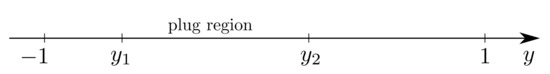
Figure 2. Plug region in Case 1; if $-B<C_0<B$ then $y_1<0<y_2$.

Case 2.

Let us consider now the second case: $-B<t_{12}(-1)<B$.

This condition furnishes

$$\begin{array}{c}\hfill \frac{\lambda }{4}-1-B<C_0<\frac{\lambda }{4}-1+B\end{array}$$

(24)

that we must associate to

$$\begin{array}{c}\hfill -\frac{1}{\lambda }-B<C_0<\frac{\lambda }{4}+1-B\end{array}$$

(25)

which assures the existence of $y_2$.

Since $t_{12}(-1)>-B$, there exists a plug region near the wall $y=-1$. In this region denoted by $[-1,y_0]$, the velocity vanishes and $t_{12}\left(y_0\right)=B$. This latter equation furnishes two real roots provided $C_0>-\frac{1}{\lambda }+B$ and $y_0$ is the smallest root given by

$$\begin{array}{c}\hfill y_0=\frac{2}{\lambda }\left[-1-\sqrt{1+\lambda (C_0-B)}\right].\end{array}$$

(26)

Taking into account these results, the condition on $C_0$ given by (25) becomes

$$\begin{array}{c}\hfill -\frac{1}{\lambda }+B<C_0<\frac{\lambda }{4}+1-B.\end{array}$$

(27)

From (27), we deduce the following condition on the Bingham number

$$\begin{array}{c}\hfill B<\frac{{(\lambda +2)}^2}{8\lambda };\end{array}$$

(28)

moreover since $y_0>-1$ after some calculations we find

$$\begin{array}{c}\hfill \lambda >2.\end{array}$$

(29)

Now, we study the flow in $[y_0,y_1]$ where

$$y_1=\frac{2}{\lambda }\left[-1+\sqrt{1+\lambda (C_0-B)}\right]$$

is the second root of the equation $t_{12}\left(y\right)=B$. In this interval, v is the solution of the problem

$$v^{\prime }+B=-\frac{\lambda }{4}{y}^2-y+C_0,v\left(y_0\right)=0$$

(30)

which gives

$$\begin{array}{c}\hfill v\left(y\right)=\frac{y_0-y}{12}[\lambda y^2+(\lambda y_0+6)y+\lambda y_0(y_0+3y_1)+6y_0],\forall y\in [y_0,y_1].\end{array}$$

(31)

Finally, we have to determine $C_0$ by requiring $v\left(y_1\right)=v\left(y_2\right)$, from which follows

$$\begin{array}{c}\hfill \lambda [2y_2^3-3y_2^2+(y_1-y_0)(y_0^2+4y_0{y}_1+y_1^2)+1]+6[{(y_2-1)}^2+y_1^2-y_0^2]=0.\end{array}$$

(32)

Inequalities (24) and (27) may be summarized in the form

$$\begin{array}{c}\hfill max\{-\frac{1}{\lambda }+B,\frac{\lambda }{4}-1-B\}<C_0<min\{\frac{\lambda }{4}-1+B,\frac{\lambda }{4}+1-B\}.\end{array}$$

(33)

We then summarize the solution of this case (Figure 3)

$$v\left(y\right)=\left\{\begin{array}{cc}0\hfill & \mathrm{if} y\in [-1,y_0](\mathrm{p}\mathrm{l}\mathrm{u}\mathrm{g} \mathrm{r}\mathrm{e}\mathrm{g}\mathrm{i}\mathrm{o}\mathrm{n}),\hfill \\ \frac{y_0-y}{12}[\lambda y^2+(\lambda y_0+6)y+\lambda y_0(y_0+3y_1)+6y_0]\hfill & \mathrm{if} y\in (y_0,y_1),\hfill \\ {(y_2-1)}^2\frac{\lambda +2\lambda y_2+6}{12}\hfill & \mathrm{if} y\in [y_1,y_2](\mathrm{p}\mathrm{l}\mathrm{u}\mathrm{g} \mathrm{r}\mathrm{e}\mathrm{g}\mathrm{i}\mathrm{o}\mathrm{n}),\hfill \\ \frac{1-y}{12}\left[\lambda y^2+(\lambda +6)y+\lambda (1-3y_2^2)+6(1-2y_2)\right]\hfill & \mathrm{if} y\in (y_2,1].\hfill \end{array}\right.$$

(34)

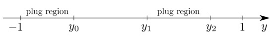
Figure 3. Plug regions in Case 2; $y_0<0$ and if $-B<C_0<B$ then $y_0<y_1<0<y_2$.

We now discuss the consequences of inequalities (33), taking into account the four possibilities and inequalities (28) and (29).

First, we assume that the max in (33) is given by ${\displaystyle -\frac{1}{\lambda }+B}$. If the min in (33) is ${\displaystyle \frac{\lambda }{4}-1+B}$, then we must have

$${\displaystyle \frac{{(\lambda -2)}^2}{8\lambda }<B<1,2<\lambda <6+4\sqrt{2}.}$$

If the min in (33) is ${\displaystyle \frac{\lambda }{4}+1-B}$, then, recalling that $\lambda >2$, we deduce

$$\mathrm{if}2<\lambda \le 6+4\sqrt{2},\mathrm{then}1\le B<\frac{{(\lambda +2)}^2}{8\lambda },$$

$$\mathrm{if}\lambda >6+4\sqrt{2},\mathrm{then}\frac{{(\lambda -2)}^2}{8\lambda }<B<\frac{{(\lambda +2)}^2}{8\lambda }.$$

Alternatively, we suppose that the max in (33) is given by ${\displaystyle \frac{\lambda }{4}-1-B}$. If the min in (33) is given by ${\displaystyle \frac{\lambda }{4}-1+B}$, then we obtain

$$\mathrm{if}2<\lambda <6+4\sqrt{2},\mathrm{then}B\le \frac{{(\lambda -2)}^2}{8\lambda },$$

$$\mathrm{if}\lambda \ge 6+4\sqrt{2},\mathrm{then}B<1.$$

Finally, if min in (33) is given by ${\displaystyle \frac{\lambda }{4}+1-B}$, then we have

$$1\le B\le \frac{{(\lambda -2)}^2}{8\lambda },\lambda \ge 6+4\sqrt{2}.$$

Moreover, we notice that $y_0<0$ and if $-B<C_0<B$ then $y_1<0<y_2$.

Case 3.

We suppose $t_{12}(-1)<-B$.

This inequality, together with the condition for the existence of $y_2$, implies that $C_0$ must satisfy

$$\begin{array}{c}\hfill -\frac{1}{\lambda }-B<C_0<\frac{\lambda }{4}-1-B.\end{array}$$

(35)

We search now for the smallest $y_0$ such that $t_{12}\left(y_0\right)=-B$. A simple calculation furnishes

$$\begin{array}{c}\hfill y_0=-\frac{2}{\lambda }\left[1+\sqrt{1+\lambda (C_0+B)}\right].\end{array}$$

(36)

We have that $y_0>-1$ if $\lambda >2$.

We solve in $[-1,y_0]$ the problem

$$v^{\prime }-B=-\frac{\lambda }{4}{y}^2-y+C_0,v(-1)=0$$

(37)

from which we get

$$\begin{array}{c}\hfill v\left(y\right)=\frac{1+y}{12}[-\lambda y^2+(\lambda -6)y+\lambda (3y_0^2-1)+6(2y_0+1)].\end{array}$$

(38)

The plug region is $[y_0,y_1]$ with

$${\displaystyle t_{12}\left(y_1\right)=B,y_1=-\frac{2}{\lambda }\left[1+\sqrt{1+\lambda (C_0-B)}\right],}$$

provided ${\displaystyle C_0>B-\frac{1}{\lambda }}$. Therefore, conditions (35) must be replaced with

$$\begin{array}{c}\hfill -\frac{1}{\lambda }+B<C_0<\frac{\lambda }{4}-1-B\end{array}$$

(39a)

$$\begin{array}{c}\hfill \Rightarrow B<\frac{{(\lambda -2)}^2}{8\lambda }.\end{array}$$

(39b)

In $[y_0,y_1]$, the velocity takes the negative constant value $v\left(y_0\right)\forall \lambda >2$, as it is easy to verify.

At this stage, we search the interval $[y_1,{\overline{y}}_1]$ where $v^{\prime }>0$ and ${\overline{y}}_1$ ($<y_2$) is such that $t_{12}\left({\overline{y}}_1\right)=B$. This latter condition gives

$${\displaystyle {\overline{y}}_1=\frac{2}{\lambda }\left[-1+\sqrt{1+\lambda (C_0-B)}\right].}$$

The velocity is found solving in the interval $[y_1,{\overline{y}}_1]$ the problem

$$v^{\prime }+B=-\frac{\lambda }{4}{y}^2-y+C_0,v\left(y_1\right)=v\left(y_0\right),$$

(40)

where $v\left(y_0\right)$ is computed using (38).

So, in the interval $[y_1,{\overline{y}}_1]$, the velocity is given by

$$\begin{array}{cc}\hfill & v\left(y\right)=-\frac{\lambda }{12}(1+y^3)+\frac{1}{2}(1-y^2)+(\frac{\lambda }{4}{y}_1^2+y_1)y+\frac{1}{2}(y_0^2-y_1^2)+\frac{\lambda }{6}(y_0^3-y_1^3)+\frac{\lambda }{4}{y}_0(y_0^2+1).\hfill \end{array}$$

(41)

In order to determine the constant $C_0$, we have to solve the equation

$$v\left(y_2\right)=v\left({\overline{y}}_1\right)$$

where $v\left(y_2\right)$ is furnished by (12) with $y_2$ given by (13): i.e.,

$$\lambda [{(y_2-1)}^2(2y_2+1)+{\overline{y}}_1({\overline{y}}_1^2-3y_1^2)+2y_1^3-5y_0^3-3y_0+1]+6[{(1-y_2)}^2+{({\overline{y}}_1-y_1)}^2-y_0^2-1]=0.$$

(42)

Moreover, we notice that $y_0<y_1<0$, and if $-B<C_0<B$, then ${\overline{y}}_1<0<y_2$.

Finally, we write the solution of this case (Figure 4)

$$v\left(y\right)=\left\{\begin{array}{cc}\frac{1+y}{12}[-\lambda y^2+(\lambda -6)y+\lambda (3y_0^2-1)+6(2y_0+1)]\hfill & \mathrm{if} y\in [-1,y_0),\hfill \\ {(y_0+1)}^2\frac{2\lambda y_0-\lambda +6}{12}\hfill & \mathrm{if} y\in [y_0,y_1](\mathrm{p}\mathrm{l}\mathrm{u}\mathrm{g} \mathrm{r}\mathrm{e}\mathrm{g}\mathrm{i}\mathrm{o}\mathrm{n}),\hfill \\ -\frac{\lambda }{12}(1+y^3)+\frac{1}{2}(1-y^2)+(\frac{\lambda }{4}{y}_1^2+y_1)y+\frac{1}{2}(y_0^2-y_1^2)+\frac{\lambda }{6}(y_0^3-y_1^3)+\frac{\lambda }{4}{y}_0(y_0^2+1)\hfill & \mathrm{if} y\in (y_1,{\overline{y}}_1),\hfill \\ {(y_2-1)}^2\frac{\lambda +2\lambda y_2+6}{12}\hfill & \mathrm{if} y\in [{\overline{y}}_1,y_2](\mathrm{p}\mathrm{l}\mathrm{u}\mathrm{g} \mathrm{r}\mathrm{e}\mathrm{g}\mathrm{i}\mathrm{o}\mathrm{n}),\hfill \\ \frac{1-y}{12}\left[\lambda y^2+(\lambda +6)y+\lambda (1-3y_2^2)+6(1-2y_2)\right]\hfill & \mathrm{if} y\in (y_2,1].\hfill \end{array}\right.$$

(43)

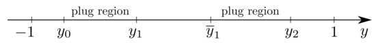
Figure 4. Plug regions in Case 3; $y_0<y_1$ and if $-B<C_0<B$, then $y_0<y_1<{\overline{y}}_1<0<y_2$.

Remark 1.

It is interesting to observe that, since $v\left(y_0\right)<0$, in case 3, the phenomenon of reverse flow occurs at the cold wall.

Remark 2.

Case 1 is possible only if $B<1$ without a priori restrictions on λ, whereas cases 2 and 3 are possible only if $\lambda >2$ while B may also assume values $\ge 1$. Thus, we have that the restrictions on B are weaker than those of the isothermal case and the natural convection ([1,4,8]).

Remark 3.

We underline that the conditions on B and λ are only necessary if it is essential that there exists $C_0$ solution of (21), or (33), or (42) satisfying the restrictions (17), or (27), or (39a), respectively.

3.1. Trend of the Velocity

In this subsection, we analyze the velocity and of the plug regions in the previous three cases.

Table 1 and Figure 5 show that for every $(\lambda ,B)$, only one of the three cases occurs.

Table 1. Values of $C_0$ and of the boundaries of the plug regions when $\lambda$ and B vary.

$\mathit{\lambda }$	B	Case	${\mathit{C}}_0$	${\mathit{y}}_0$	${\mathit{y}}_1$	${\overline{\mathit{y}}}_1$	${\mathit{y}}_2$
1.0	0.10	1	0.0923		−0.0077		0.1838
1.0	0.50	1	0.1441		−0.3948		0.5645
1.0	0.90	1	0.2245		−0.8607		0.9151
3.0	0.10	1	0.2732		0.1551		0.3039
3.0	0.50	1	0.4007		−0.1080		0.6161
3.0	0.90	2	0.6063	−0.8964	−0.4369		0.8995
3.0	1.0	2	0.6748	−0.7710	−0.5623		0.9697
5.0	0.10	1	0.4486		0.2625		0.3739
5.0	0.50	2	0.6082	−0.8966	0.0966		0.6230
5.0	1.0	2	0.8685	−0.6340	−0.1660		0.8864
5.0	1.20	2	1.0040	−0.4567	−0.3433		0.9868
7.0	0.10	3	0.6148	−0.9858	−0.8988	0.3273	0.4144
7.0	0.50	2	0.7716	−0.7724	0.2010		0.6133
7.0	1.0	2	1.0145	−0.5856	0.0142		0.8246
7.0	1.20	2	1.1306	−0.4905	−0.0809		0.9031
10.0	0.10	3	0.8570	−0.8502	−0.7855	0.3855	0.4502
10.0	0.50	3	0.9865	−0.9966	−0.6844	0.2844	0.5966
10.0	0.70	2	1.0721	−0.6345	0.2345		0.6653
10.0	1.20	2	1.3162	−0.4941	0.0941		0.8230

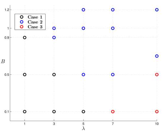
Figure 5. The position of the points in parameter space indicates which case occurs. The picture shows only the couples $(\lambda ,B)$ of Table 1.

The profile of the velocity in Case 1 is plotted in Figure 6: v decreases as B increases and the maximum of the velocity increases as $\lambda$ increases.

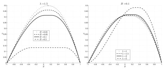
Figure 6. Case 1: profile of the velocity.

In this case, the plug region is closer to the hot wall; its boundaries are shown in Figure 7. We have that $y_1$ decreases with B and increases with $\lambda$, while $y_2$ increases with B and $\lambda$. Hence, when B increases, the thickness of the plug region increases.

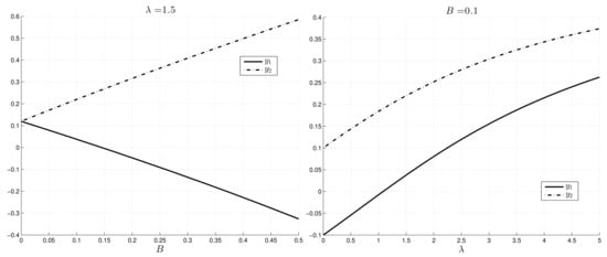
Figure 7. Case 1: plug boundaries ($y_1$, $y_2$).

Figure 8 shows the trend of v as the Bingham number B and the buoyancy parameter $\lambda$ vary in Case 2: the velocity decreases as B increases, as in Case 1.

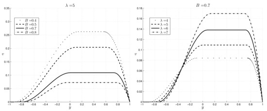
Figure 8. Case 2: profile of the velocity.

In Case 2, we have two plug regions (Figure 9): one attached to the cold wall ($[0,y_0]$) and one closer to the hot wall ($[y_1,y_2]$).

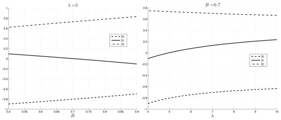
Figure 9. Case 2: plug boundaries ($y_0$, $y_1$, $y_2$).

We have that $y_0$ increases with B and $\lambda$ such that the thickness of the plug region $[0,y_0]$ increases with these two parameters. Furthermore, we see that the thickness of the plug region $[y_1,y_2]$ increases with B and decreases with $\lambda$.

Finally, the behavior of the velocity in Case 3 is shown in Figure 10, which underlines that, in this case, the reverse flow phenomenon can occur near the cold wall. This phenomenon has been studied in other physical situations (see, for example, [7,14,15]). This situation occurs when the magnitude of the buoyancy parameter $\lambda$ is large enough ($\lambda >6$). We notice that the reverse flow occurs for a Bingham fluid if $\lambda$ takes values greater than those concerning Newtonian fluids for which the critical value of $\lambda$ is 6 ([15]). This fact is physically reasonable.

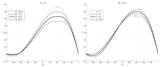
Figure 10. Case 3: profile of the velocity.

We recall that now we have two plug regions: the thickness of $[y_0,y_1]$ and $[{\overline{y}}_1,y_2]$ increases with B, while slightly decreases with $\lambda$ (Figure 11).

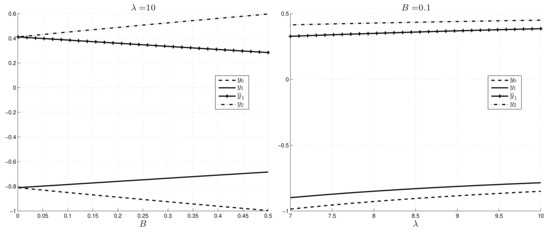
Figure 11. Case 3: plug boundaries ($y_0$, $y_1$, ${\overline{y}}_1$, $y_2$).

4. Hartmann Flow with Mixed Convection

In this section, we assume that the Bingham fluid filling the channel $\mathcal{S}$ is electrically conducting, in the regions outside $\mathcal{S}$ there is a vacuum, and the walls are nonelectrically conducting.

An external uniform magnetic field ${\mathbf{H}}_0=H_0{\mathbf{e}}_2$ normal to planes ${\mathrm{\Pi }}_{1,2}$ ($H_0>0$) is applied.

We search the magnetic field $\mathbf{H}\in C^2\left(\mathcal{S}\right)$ in the form:

$$\begin{array}{c}\hfill \mathbf{H}=H_1\left(x_2\right){\mathbf{e}}_1+H_0{\mathbf{e}}_2,\end{array}$$

(44)

so that $\mathbf{H}$ is divergence free.

The equations governing the motion now are

$$\begin{array}{c}{\rho }_0\mathbf{v}·\nabla \mathbf{v}=-\nabla p+\nabla ·{\mathbf{T}}^D+{\mu }_e(\nabla \times \mathbf{H})\times \mathbf{H}+{\rho }_0[1-\alpha (T-T_0)]\mathbf{g},\hfill \end{array}$$

(45a)

$$\begin{array}{c}\nabla ·\mathbf{v}=0,\nabla ·\mathbf{H}=0,\hfill \end{array}$$

(45b)

$$\begin{array}{c}{\eta }_e\Delta \mathbf{H}+\nabla \times (\mathbf{v}\times \mathbf{H})=\mathbf{0},\hfill \end{array}$$

(45c)

$$\begin{array}{c}\nabla T·\mathbf{v}=b\Delta T\hfill \end{array}$$

(45d)

where ${\mu }_e,{\eta }_e$ are the magnetic permeability, magnetic diffusivity respectively (positive constants).

Boundary conditions for the induced magnetic field $H_1$ are

$$H_1(\pm d)=0.$$

(46)

As in the previous section, we write the problem in dimensionless form by adding to (7) relation giving the rescaled induced magnetic field

$$h\left(y\right)=\frac{H_1\left(dy\right)}{V_0\sqrt{{\sigma }_e\mu }},{\sigma }_e=\mathrm{e}\mathrm{l}\mathrm{e}\mathrm{c}\mathrm{t}\mathrm{r}\mathrm{i}\mathrm{c}\mathrm{a}\mathrm{l}\mathrm{c}\mathrm{o}\mathrm{n}\mathrm{d}\mathrm{u}\mathrm{c}\mathrm{t}\mathrm{i}\mathrm{v}\mathrm{i}\mathrm{t}\mathrm{y}.$$

(47)

By virtue of (3), (44), and (45a), we deduce

$$\begin{array}{cc}\hfill & P=P\left(x_1\right)=-C{x}_1+p_{0}C,p_0\mathrm{s}\mathrm{o}\mathrm{m}\mathrm{e}\mathrm{c}\mathrm{o}\mathrm{n}\mathrm{s}\mathrm{t}\mathrm{a}\mathrm{n}\mathrm{t}\mathrm{s},\hfill \\ \hfill & T_{12}^D=T_{21}^D=-{\mu }_e{H}_0{H}_1\left(x_2\right)-C{x}_2+{\tilde{C}}_0,T_{ij}^D=0\mathrm{for}i,j\ne 1,2\hfill \end{array}$$

(48)

where ${\displaystyle P=p+{\rho }_{0}g{x}_1+{\mu }_e\frac{H_1^2}{2}}$ is the modified pressure, $C>0$ and ${\tilde{C}}_0$ is an integration constant.

Using (7) and (47) and introducing the Hartmann number M given by

$${\displaystyle M=d{\mu }_e{H}_0\sqrt{\frac{{\sigma }_e}{\mu }},}$$

we have that the only significant component of ${\mathbf{T}}^D$ is

$$\begin{array}{c}\hfill t_{12}=-Mh-\frac{\lambda }{4}{y}^2-y+C_0.\end{array}$$

(49)

Then, outside the plug regions, we have the system

$$\begin{array}{cc}\hfill & v^{\prime }\pm B=-Mh-\frac{\lambda }{4}{y}^2-y+C_0,\hfill \\ \hfill & h^{″}+M{v}^{\prime }=0,\hfill \end{array}$$

while the dimesionless temperature $\vartheta$ is again given by ${\displaystyle \vartheta \left(y\right)=\frac{y}{2}.}$

In order to study the flow, we adopt arguments and procedures analogous to those used in the absence of magnetic field. However, as it is seen from (49), now $t_{12}$ depends on h which is unknown so that we cannot obtain the explicit expressions of the boundaries of the plug regions in terms of $B,C_0,\lambda$ as in Section 3. For this reason, it is not possible to find a priori restrictions on the buoyancy parameter $\lambda$.

As in the previous section, we assume $t_{12}\left(1\right)<-B$ so that from (46) and (49), we obtain again condition (10b) on the integration constant $C_0$.

The hypothesis on $t_{12}\left(1\right)$ assures that near the hot wall $y=1$, there is a region where the continuum behaves as a fluid.

We denote by $[y_2,1]$ this region with $y_2$ such that $t_{12}\left(y_2\right)=-B$. Then, we have to solve in this interval the system

$$\begin{array}{cc}\hfill & v^{\prime }-B=-Mh-\frac{\lambda }{4}{y}^2-y+C_0,\hfill \end{array}$$

(50a)

$$\begin{array}{cc}\hfill & h^{″}+M{v}^{\prime }=0\hfill \end{array}$$

(50b)

with the boundary conditions

$$\begin{array}{cc}\hfill & v\left(1\right)=0,v^{\prime }\left(y_2\right)=0,h\left(1\right)=0.\hfill \end{array}$$

(51)

The solution is given by

$$\begin{array}{cc}\hfill & v\left(y\right)=-c_{1}sinh\left(My\right)-c_{2}cosh\left(My\right)+\frac{\lambda }{2M^2}y+c_3,\hfill \end{array}$$

(52a)

$$\begin{array}{cc}\hfill & h\left(y\right)=c_{1}cosh\left(My\right)+c_{2}sinh\left(My\right)-\frac{\lambda }{4M}{y}^2-\frac{y}{M}+\frac{B+C_0}{M}-\frac{\lambda }{2M^3}\forall y\in [y_2,1]\hfill \end{array}$$

(52b)

where the constants $c_1,c_2,c_3$ depend on $C_0,y_2$, which, for the moment, are unknown. The expressions of $c_1,c_2,c_3$ are given in the Appendix A.

In order to study the flow in $[-1,y_2]$, we have to distinguish the same three cases examined in the absence of the magnetic field.

Case 1M: $t_{12}(-1)>B$

This condition together (10b) furnishes

$$\begin{array}{c}\hfill \frac{\lambda }{4}+B-1<C_0<\frac{\lambda }{4}-B+1,B<1.\end{array}$$

(53)

Now, we search $y_1\in (-1,y_2)$ such that $t_{12}\left(y_1\right)=B$ and in $[-1,y_1]$ the continuum behaves as a fluid. Therefore, in this interval, we have to solve the system

$$\begin{array}{cc}\hfill & v^{\prime }+B=-Mh-\frac{\lambda }{4}{y}^2-y+C_0,\hfill \\ \hfill & h^{″}+M{v}^{\prime }=0\hfill \end{array}$$

(54)

with the boundary conditions

$$\begin{array}{cc}\hfill & v(-1)=0,v^{\prime }\left(y_1\right)=0,h(-1)=0.\hfill \end{array}$$

(55)

The solution is

$$\begin{array}{cc}\hfill & v\left(y\right)=-c_{4}sinh\left(My\right)-c_{5}cosh\left(My\right)+\frac{\lambda }{2M^2}y+c_6,\hfill \\ \hfill & h\left(y\right)=c_{4}cosh\left(My\right)+c_{5}sinh\left(My\right)-\frac{\lambda }{4M}{y}^2-\frac{y}{M}+\frac{C_0-B}{M}-\frac{\lambda }{2M^3}\forall y\in [-1,y_1]\hfill \end{array}$$

(56)

where the constants $c_4,c_5,c_6$ are given in the Appendix A and they depend on $C_0,y_1$ which for the moment are unknown.

Unlike what happens in the absence of the magnetic field, $y_1$ and $y_2$ cannot be determined explicitly as function of $C_0$ (see (13) and (18)) so that we have three unknowns $y_1,y_2,C_0$ that we can determine by means of the following arguments.

First of all, we have that $[y_1,y_2]$ is a plug region so that

$$\begin{array}{c}\hfill v\left(y_1\right)=v\left(y_2\right).\end{array}$$

(57)

Moreover, also in this region Equation (50b) holds; hence, $h^{″}=0$ from which $h^{\prime }\left(y\right)=h^{\prime }\left(y_1\right)=h^{\prime }\left(y_2\right)\forall y\in [y_1,y_2]$. Then the induced magnetic field in the plug region is linear. Precisely, we have

$$\begin{array}{c}\hfill h\left(y\right)=h^{\prime }\left(y_1\right)y+h\left(y_2\right)-h^{\prime }\left(y_2\right)y_2\Rightarrow h\left(y_1\right)-h^{\prime }\left(y_1\right)y_1=h\left(y_2\right)-h^{\prime }\left(y_2\right)y_2.\end{array}$$

(58)

Finally, since $h^{\prime }+Mv=\mathrm{constant}$ in $[-1,1]$, then

$$\begin{array}{c}\hfill h^{\prime }(-1)=h^{\prime }\left(1\right).\end{array}$$

(59)

Taking into account (57)–(59), we have that $y_1,y_2,C_0$ are determined by solving the system

$$\begin{array}{cc}\hfill & \frac{\lambda [M^2+2-2cosh\left(M(1+y_1)\right)]-4M^2(C_0-B+1)}{sinh\left(M(1+y_1)\right)}+\hfill \\ \hfill & \frac{\lambda [M^2+2-2cosh\left(M(1-y_2)\right)]-4M^2(C_0+B-1)}{sinh\left(M(1-y_2)\right)}+2\lambda M(y_1-y_2)=0,\hfill \\ \hfill & y_1\frac{\lambda [M^2+2-2cosh\left(M(1+y_1)\right)]-4M^2(C_0-B+1)}{sinh\left(M(1+y_1)\right)}+\hfill \\ & +y_2\frac{\lambda [M^2+2-2cosh\left(M(1-y_2)\right)]-4M^2(C_0+B-1)}{sinh\left(M(1-y_2)\right)}+\lambda M(y_1^2-y_2^2)-8MB=0,\hfill \\ \hfill & \frac{\lambda [2-(M^2+2)cosh\left(M(1+y_1)\right)]+4M^2(C_0-B+1)cosh\left(M(1+y_1)\right)}{sinh\left(M(1+y_1)\right)}+\hfill \\ & +\frac{\lambda [2-(M^2+2)cosh\left(M(1-y_2)\right)]+4M^2(C_0+B-1)cosh\left(M(1-y_2)\right)}{sinh\left(M(1-y_2)\right)}+4M\lambda =0.\hfill \end{array}$$

(60)

We now summarize the solution of this case (Figure 2)

$$v\left(y\right)=\left\{\begin{array}{cc}-c_{4}sinh\left(My\right)-c_{5}cosh\left(My\right)+\frac{\lambda }{2M^2}y+c_6\hfill & \mathrm{if} y\in [-1,y_1),\hfill \\ -c_{4}sinh\left(M{y}_1\right)-c_{5}cosh\left(M{y}_1\right)+\frac{\lambda }{2M^2}{y}_1+c_6\hfill & \mathrm{if} y\in [y_1,y_2](\mathrm{p}\mathrm{l}\mathrm{u}\mathrm{g} \mathrm{r}\mathrm{e}\mathrm{g}\mathrm{i}\mathrm{o}\mathrm{n}),\hfill \\ -c_{1}sinh\left(My\right)-c_{2}cosh\left(My\right)+\frac{\lambda }{2M^2}y+c_3\hfill & \mathrm{if} y\in (y_2,1];\hfill \end{array}\right.$$

(61)

$$h\left(y\right)=\left\{\begin{array}{cc}{c}_{4}cosh\left(My\right)+c_{5}sinh\left(My\right)-\frac{\lambda }{4M}{y}^2-\frac{y}{M}+\frac{C_0-B}{M}-\frac{\lambda }{2M^3}\hfill & \mathrm{if} y\in [-1,y_1),\hfill \\ h^{\prime }\left(y_1\right)y+h\left(y_2\right)-h^{\prime }\left(y_2\right)y_2\hfill & \mathrm{if} y\in [y_1,y_2](\mathrm{p}\mathrm{l}\mathrm{u}\mathrm{g} \mathrm{r}\mathrm{e}\mathrm{g}\mathrm{i}\mathrm{o}\mathrm{n}),\hfill \\ c_{1}cosh\left(My\right)+c_{2}sinh\left(My\right)-\frac{\lambda }{4M}{y}^2-\frac{y}{M}+\frac{B+C_0}{M}-\frac{\lambda }{2M^3}\hfill & \mathrm{if} y\in (y_2,1].\hfill \end{array}\right.$$

(62)

Case 2M: $-B<t_{12}(-1)<B$

This condition on $t_{12}$ furnishes again (24). Since inequality (10b) holds, we have to distinguish two cases:

$$\begin{array}{cc}\hfill & B<1\Rightarrow \frac{\lambda }{4}-1-B<C_0<\frac{\lambda }{4}-1+B\hfill \\ \hfill & B\ge 1\Rightarrow \frac{\lambda }{4}-1-B<C_0<\frac{\lambda }{4}+1-B.\hfill \end{array}$$

(63)

Since $t_{12}(-1)>-B$, there is a plug region near the cold wall. We denote by $[-1,y_0]$ this region where $v=0$; $y_0<y_2$ is the smallest solution of the equation $t_{12}\left(y\right)=B$, i.e.,

$$\begin{array}{c}\hfill Mh\left(y_0\right)+\frac{\lambda }{4}{y}_0^2+y_0-C_0+B=0.\end{array}$$

(64)

As far as the expression of the induced magnetic field is concerned, from $h^{″}=0$ we deduce easily

$$\begin{array}{c}\hfill h\left(y\right)=h^{\prime }\left(y_0\right)(y+1)\forall y\in [-1,y_0].\end{array}$$

(65)

Of course, $h^{\prime }\left(y_0\right)=h^{\prime }(-1)$ and $h^{\prime }(-1)=h^{\prime }\left(1\right)$ as we have explained in the Case 1.

Now, we suppose $y>y_0$. By virtue of the continuity of v and taking into account that $v\ne 0$ in $[y_2,1)$ we search $y_1$ such that $v\ne 0$ in $(y_0,y_1]$. As in the Section 2 we have that $y_1(<y_2)$ is solution of the equation $t_{12}\left(y\right)=B$.

Therefore, we have to solve the system (54) with the boundary conditions

$$\begin{array}{cc}\hfill & v\left(y_0\right)=0,v^{\prime }\left(y_1\right)=0,h\left(y_0\right)=-\frac{1}{M}\left(\frac{\lambda }{4}{y}_0^2+y_0-C_0+B\right).\hfill \end{array}$$

(66)

The solution is given by

$$\begin{array}{cc}\hfill & v\left(y\right)=-c_{7}sinh\left(My\right)-c_{8}cosh\left(My\right)+\frac{\lambda }{2M^2}y+c_9,\hfill \end{array}$$

(67a)

$$\begin{array}{cc}\hfill & h\left(y\right)=c_{7}cosh\left(My\right)+c_{8}sinh\left(My\right)-\frac{\lambda }{4M}{y}^2-\frac{y}{M}+\frac{C_0-B}{M}-\frac{\lambda }{2M^3}\forall y\in [y_0,y_1]\hfill \end{array}$$

(67b)

where the constants appearing in the solution have the expressions given in (A3).

Finally, in $[y_1,y_2]$ the velocity is constant, i.e., $v\left(y\right)=v\left(y_1\right)=v\left(y_2\right)$ and the induced magnetic field is linear and given by $h\left(y\right)=h^{\prime }\left(y_1\right)y+[h\left(y_2\right)-h^{\prime }\left(y_2\right)y_2]$.

At this stage, we must determine $y_0,y_1,y_2,C_0$ by means of the system

$$\begin{array}{cc}\hfill & v\left(y_1\right)=v\left(y_2\right),h\left(y_0\right)=h^{\prime }\left(y_0\right)(y_0+1),\hfill \\ \hfill & h^{\prime }\left(y_0\right)=h^{\prime }\left(1\right),h\left(y_1\right)-h^{\prime }\left(y_1\right)y_1=h\left(y_2\right)-h^{\prime }\left(y_2\right)y_2\hfill \end{array}$$

(68)

where $h\left(y_0\right)$ is given in (66), $h^{\prime }\left(y_0\right)$ and $h^{\prime }\left(1\right)$ are obtained from (67b) and (52b). If we explicit Equation (68), then we get

$$\begin{array}{cc}\hfill & \frac{\lambda [M^2+2-2cosh\left(M(1-y_2)\right)]-4M^2(C_0+B-1)}{sinh\left(M(1-y_2)\right)}+\hfill \\ \hfill & 2\lambda \frac{1-cosh\left(M(y_1-y_0)\right)}{sinh\left(M(y_1-y_0)\right)}+2\lambda M(y_1-y_0)=0,\hfill \\ \hfill & \frac{2\lambda (y_0+1)[1-cosh\left(M(y_1-y_0)\right)}{sinh\left(M(y_1-y_0)\right)}-\lambda M{y}_0(y_0+2)-4M(C_0-B+1)=0,\hfill \\ \hfill & \frac{\lambda [2-(M^2+2)cosh\left(M(1-y_2)\right)]+4M^2(C_0+B-1)cosh\left(M(1-y_2)\right)}{sinh\left(M(1-y_2)\right)}+\hfill \\ & +2\lambda \frac{1-cosh\left(M(y_1-y_0)\right)}{sinh\left(M(y_1-y_0)\right)}+2\lambda M(1-y_0)=0,\hfill \\ \hfill & y_2\frac{\lambda [M^2+2-2cosh\left(M(1-y_2)\right)]-4M^2(C_0+B-1)}{sinh\left(M(1-y_2)\right)}+\hfill \\ & +y_1\frac{2\lambda [1-cosh\left(M(y_1-y_0)\right)]}{sinh\left(M(y_1-y_0)\right)}+\lambda M(y_1^2-y_2^2)-8MB=0.\hfill \end{array}$$

(69)

We now summarize the solution of this case (Figure 3)

$$v\left(y\right)=\left\{\begin{array}{cc}0\hfill & \mathrm{if} y\in [-1,y_0](\mathrm{p}\mathrm{l}\mathrm{u}\mathrm{g} \mathrm{r}\mathrm{e}\mathrm{g}\mathrm{i}\mathrm{o}\mathrm{n}),\hfill \\ -c_{7}sinh\left(My\right)-c_{8}cosh\left(My\right)+\frac{\lambda }{2M^2}y+c_9\hfill & \mathrm{if} y\in (y_0,y_1),\hfill \\ -c_{7}sinh\left(M{y}_1\right)-c_{8}cosh\left(M{y}_1\right)+\frac{\lambda }{2M^2}{y}_1+c_9\hfill & \mathrm{if} y\in [y_1,y_2](\mathrm{p}\mathrm{l}\mathrm{u}\mathrm{g} \mathrm{r}\mathrm{e}\mathrm{g}\mathrm{i}\mathrm{o}\mathrm{n}),\hfill \\ -c_{1}sinh\left(My\right)-c_{2}cosh\left(My\right)+\frac{\lambda }{2M^2}y+c_3\hfill & \mathrm{if} y\in (y_2,1];\hfill \end{array}\right.$$

(70)

$$h\left(y\right)=\left\{\begin{array}{cc}{h}^{\prime }\left(y_0\right)(y+1)\hfill & \mathrm{if} y\in [-1,y_0](\mathrm{p}\mathrm{l}\mathrm{u}\mathrm{g} \mathrm{r}\mathrm{e}\mathrm{g}\mathrm{i}\mathrm{o}\mathrm{n}),\hfill \\ c_{7}cosh\left(My\right)+c_{8}sinh\left(My\right)-\frac{\lambda }{4M}{y}^2-\frac{y}{M}+\frac{C_0-B}{M}-\frac{\lambda }{2M^3}\hfill & \mathrm{if} y\in (y_0,y_1),\hfill \\ h^{\prime }\left(y_1\right)y+h\left(y_2\right)-h^{\prime }\left(y_2\right)y_2\hfill & \mathrm{if} y\in [y_1,y_2](\mathrm{p}\mathrm{l}\mathrm{u}\mathrm{g} \mathrm{r}\mathrm{e}\mathrm{g}\mathrm{i}\mathrm{o}\mathrm{n}),\hfill \\ c_{1}cosh\left(My\right)+c_{2}sinh\left(My\right)-\frac{\lambda }{4M}{y}^2-\frac{y}{M}+\frac{B+C_0}{M}-\frac{\lambda }{2M^3}\hfill & \mathrm{if} y\in (y_2,1].\hfill \end{array}\right.$$

(71)

Case 3M: $t_{12}(-1)<-B$

In this case, the condition on $t_{12}(-1)$ furnishes

$$\begin{array}{c}\hfill C_0<\frac{\lambda }{4}-1-B.\end{array}$$

(72)

Now, we study the flow in $[-1,y_2]$; first of all we search the smallest $y_0\in (-1,y_2)$ such that $t_{12}\left(y_0\right)=-B$, i.e.,

$$\begin{array}{c}\hfill Mh\left(y_0\right)+\frac{\lambda }{4}{y}_0^2+y_0-C_0-B=0.\end{array}$$

(73)

We have to solve in $[-1,y_0]$ the system (50) with the boundary conditions

$$\begin{array}{cc}\hfill & v(-1)=0,v^{\prime }\left(y_0\right)=0,h(-1)=0\hfill \end{array}$$

(74)

whose solution is

$$\begin{array}{cc}\hfill & v\left(y\right)=-c_{10}sinh\left(My\right)-c_{11}cosh\left(My\right)+\frac{\lambda }{2M^2}y+c_{12},\hfill \\ \hfill & h\left(y\right)=c_{10}cosh\left(My\right)+c_{11}sinh\left(My\right)-\frac{\lambda }{4M}{y}^2-\frac{y}{M}+\frac{C_0+B}{M}-\frac{\lambda }{2M^3}\forall y\in [-1,y_0]\hfill \end{array}$$

(75)

where $c_{10},c_{11},c_{12}$ are given in the Appendix A.

Now, we search the plug region $[y_0,y_1]$ where $y_1$ satisfies the equation $t_{12}\left(y\right)=B$, i.e.,

$$\begin{array}{c}\hfill Mh\left(y_1\right)+\frac{\lambda }{4}{y}_1^2+y_1-C_0+B=0.\end{array}$$

(76)

In this interval

$$\begin{array}{c}\hfill v\left(y\right)=v\left(y_0\right)=v\left(y_1\right),h\left(y\right)=h^{\prime }\left(y_0\right)y+h\left(y_1\right)-h^{\prime }\left(y_1\right)y_1.\end{array}$$

(77)

The next step is to search the interval $[y_1,{\overline{y}}_1]$ where $v^{\prime }>0$ and ${\overline{y}}_1<y_2$ is solution of $t_{12}\left(y\right)=B$.

The velocity and the induced magnetic field satisfy in $[y_1,{\overline{y}}_1]$ the system (54) with the boundary conditions

$$\begin{array}{c}\hfill v\left(y_1\right)=v\left(y_0\right),v^{\prime }\left({\overline{y}}_1\right)=0,h\left(y_1\right)=-\frac{1}{M}\left(\frac{\lambda }{4}{y}_1^2+y_1-C_0+B\right).\end{array}$$

(78)

Hence $v,h$ are given by (67) with the substitution of the constants $c_7,c_8,c_9$ with $c_{13},c_{14},c_{15},$ respectively. In the Appendix A, we write the expressions of the arbitrary constants.

In $[{\overline{y}}_1,y_2]$ there is another plug region where

$$\begin{array}{c}\hfill v\left(y\right)=v\left({\overline{y}}_1\right)=v\left(y_2\right),h\left(y\right)=h^{\prime }\left({\overline{y}}_1\right)y+h\left(y_2\right)-h^{\prime }\left(y_2\right)y_2.\end{array}$$

(79)

To conclude, we must determine $C_0,y_0,y_1,y_2,{\overline{y}}_1$ that are unknown.

By proceeding as previously, we have to solve the system

$$\begin{array}{cc}\hfill & v\left(y_2\right)=v\left({\overline{y}}_1\right),h\left({\overline{y}}_1\right)-h^{\prime }\left({\overline{y}}_1\right){\overline{y}}_1=h\left(y_2\right)-h^{\prime }\left(y_2\right)y_2,h^{\prime }\left({\overline{y}}_1\right)+Mv\left({\overline{y}}_1\right)=h^{\prime }(-1),\hfill \\ \hfill & h^{\prime }\left(y_0\right)+Mv\left(y_0\right)=h^{\prime }\left(1\right),h\left(y_0\right)-h^{\prime }\left(y_0\right)y_0=h\left(y_1\right)-h^{\prime }\left(y_1\right)y_1.\hfill \end{array}$$

(80)

After some calculations the previous system becomes

$$\begin{array}{cc}\hfill & \frac{\lambda [M^2+2-2cosh\left(M(1-y_2)\right)]-4M^2(C_0+B-1)}{sinh\left(M(1-y_2)\right)}+\hfill \\ & +\frac{2\lambda [1-cosh\left(M({\overline{y}}_1-y_1)\right)]}{sinh\left(M({\overline{y}}_1-y_1)\right)}+2\lambda M({\overline{y}}_1-y_2)=0,\hfill \\ \hfill & y_2\frac{\lambda [M^2+2-2cosh\left(M(1-y_2)\right)]-4M^2(C_0+B-1)}{sinh\left(M(1-y_2)\right)}+\hfill \\ & +{\overline{y}}_1\frac{2\lambda [1-cosh\left(M({\overline{y}}_1-y_1)\right)]}{sinh\left(M({\overline{y}}_1-y_1)\right)}+\lambda M({\overline{y}}_1^2-y_2^2)-8MB=0,\hfill \\ \hfill & \frac{\lambda [M^2+2-2cosh\left(M(1+y_0)\right)]-4M^2(C_0+B+1)}{sinh\left(M(1+y_0)\right)}+\hfill \\ & +\frac{2\lambda [1-cosh\left(M({\overline{y}}_1-y_1)\right)]}{sinh\left(M({\overline{y}}_1-y_1)\right)}+2M\lambda (y_0-y_1)=0,\hfill \\ \hfill & \frac{\lambda [2-(M^2+2)cosh\left(M(1+y_0)\right)]+4M^2(C_0+B+1)cosh\left(M(1+y_0)\right)}{sinh\left(M(1+y_0)\right)}+\hfill \\ & +\frac{\lambda [2-(M^2+2)cosh\left(M(1-y_2)\right)]+4M^2(C_0+B-1)cosh\left(M(1-y_2)\right)}{sinh\left(M(1-y_2)\right)}+4M\lambda =0,\hfill \\ \hfill & y_0\frac{\lambda [M^2+2-2cosh\left(M(1+y_0)\right)]+4M^2(C_0+B+1)}{sinh\left(M(1+y_0)\right)}+\hfill \\ & +y_1\frac{2\lambda [1-cosh\left(M({\overline{y}}_1-y_1)\right)]}{sinh\left(M({\overline{y}}_1-y_1)\right)}+\lambda M(y_0^2-y_1^2)+8MB=0.\hfill \end{array}$$

(81)

Finally, the solution of this case is given by (Figure 4)

$$v\left(y\right)=\left\{\begin{array}{cc}-c_{10}sinh\left(My\right)-c_{11}cosh\left(My\right)+\frac{\lambda }{2M^2}y+c_{12}\hfill & \mathrm{if} y\in [-1,y_0),\hfill \\ -c_{10}sinh\left(M{y}_0\right)-c_{11}cosh\left(M{y}_0\right)+\frac{\lambda }{2M^2}{y}_0+c_{12}\hfill & \mathrm{if} y\in [y_0,y_1](\mathrm{p}\mathrm{l}\mathrm{u}\mathrm{g} \mathrm{r}\mathrm{e}\mathrm{g}\mathrm{i}\mathrm{o}\mathrm{n}),\hfill \\ -c_{13}sinh\left(My\right)-c_{14}cosh\left(My\right)+\frac{\lambda }{2M^2}y+c_{15}\hfill & \mathrm{if} y\in (y_1,{\overline{y}}_1),\hfill \\ -c_{13}sinh\left(M{\overline{y}}_1\right)-c_{14}cosh\left(M{\overline{y}}_1\right)+\frac{\lambda }{2M^2}{\overline{y}}_1+c_{15}\hfill & \mathrm{if} y\in [{\overline{y}}_1,y_2](\mathrm{p}\mathrm{l}\mathrm{u}\mathrm{g} \mathrm{r}\mathrm{e}\mathrm{g}\mathrm{i}\mathrm{o}\mathrm{n}),\hfill \\ -c_{1}sinh\left(My\right)-c_{2}cosh\left(My\right)+\frac{\lambda }{2M^2}y+c_3\hfill & \mathrm{if} y\in (y_2,1];\hfill \end{array}\right.$$

(82)

$$h\left(y\right)=\left\{\begin{array}{cc}{c}_{10}cosh\left(My\right)+c_{11}sinh\left(My\right)-\frac{\lambda }{4M}{y}^2-\frac{y}{M}+\frac{C_0+B}{M}-\frac{\lambda }{2M^3}\hfill & \mathrm{if} y\in [-1,y_0),\hfill \\ h^{\prime }\left(y_0\right)y+h\left(y_1\right)-h^{\prime }\left(y_1\right)y_1\hfill & \mathrm{if} y\in [y_0,y_1](\mathrm{p}\mathrm{l}\mathrm{u}\mathrm{g} \mathrm{r}\mathrm{e}\mathrm{g}\mathrm{i}\mathrm{o}\mathrm{n}),\hfill \\ c_{13}cosh\left(My\right)+c_{14}sinh\left(My\right)-\frac{\lambda }{4M}{y}^2-\frac{y}{M}+\frac{C_0-B}{M}-\frac{\lambda }{2M^3}\hfill & \mathrm{if} y\in (y_1,{\overline{y}}_1),\hfill \\ h^{\prime }\left(y_3\right)y+h\left(y_2\right)-h^{\prime }\left(y_2\right)y_2\hfill & \mathrm{if} y\in [{\overline{y}}_1,y_2](\mathrm{p}\mathrm{l}\mathrm{u}\mathrm{g} \mathrm{r}\mathrm{e}\mathrm{g}\mathrm{i}\mathrm{o}\mathrm{n}),\hfill \\ c_{1}cosh\left(My\right)+c_{2}sinh\left(My\right)-\frac{\lambda }{4M}{y}^2-\frac{y}{M}+\frac{B+C_0}{M}-\frac{\lambda }{2M^3}\hfill & \mathrm{if} y\in (y_2,1].\hfill \end{array}\right.$$

(83)

Remark 4.

Taking into account the Maxwell equations, we have that to the magnetic field $\mathbf{H}$ an electric field $\mathbf{E}$ is associated given by

$$\mathbf{E}=\frac{1}{{\sigma }_e}\nabla \times \mathbf{H}+{\mu }_e\mathbf{H}\times \mathbf{v}$$

which furnishes

$$\begin{array}{c}\hfill \mathbf{E}=-\frac{{\mu }_e{H}_0{V}_0}{M}[h^{\prime }\left(y\right)+Mv\left(y\right)]{\mathbf{e}}_3=E_0{\mathbf{e}}_3,\end{array}$$

where $E_0$ is a constant, as a consequence of (50b). The value taken by $E_0$ depends on the case considered.

Since in the most of papers concerning MHD flows, the induced magnetic fied is neglected, the presence of a uniform electric field orthogonal to the flow and to the magnetic field is not highlighted.

Finally, outside the walls, where we assume that there is a vacuum, the electromagnetic field is given by

$$\begin{array}{cc}\hfill \mathbf{E}& =E_0{\mathbf{e}}_3,\mathbf{H}=H_0{\mathbf{e}}_2.\hfill \end{array}$$

Remark 5.

We furnish some physical characteristics of the flow in the three cases. These features do not depend on the presence of the external magnetic field.

The Nusselt number at the walls is

$$\begin{array}{c}\hfill {Nu}_{1,2}=\frac{k_{1,2}d}{k}=\frac{d}{T_2-T_1}\frac{dT}{d{x}_2}{|}_{x_2=\pm d}={\vartheta }^{\prime }(\pm 1)=\frac{1}{2}\end{array}$$

where $k_{1,2}$ are the heat transfer coefficients of the walls.

The heat flux vector, which is related to the Nusselt number, is constant in the channel and is given by

$$\begin{array}{c}\hfill \mathbf{q}=-\frac{(T_2-T_1)k}{2d}{\mathbf{e}}_{\mathbf{2}}.\end{array}$$

This expression is physically quite reasonable because the heat transfer occurs from the hot wall to the cold one.

The skin frictions ${\mathbf{\tau }}_{1,2}$ at both walls are given by

$$\begin{array}{c}\hfill {\mathbf{\tau }}_{1,2}=\mu \frac{V_0}{d}[\mp (C_0-\frac{\lambda }{4})-1]{\mathbf{e}}_1.\end{array}$$

5. Discussion

In this section we analyze the behavior of the velocity and determine the plug regions in the three cases influenced by the presence of the external magnetic field.

In Table 2 we write which of the three cases occurs for $(M,\lambda ,B)$ fixed (we refer to Figure 12 for better viewing).

Table 2. Values of $C_0$ and of the boundaries of the plug regions when M, $\lambda$ and B vary.

M	$\mathit{\lambda }$	B	Case	${\mathit{C}}_0$	${\mathit{y}}_0$	${\mathit{y}}_1$	${\overline{\mathit{y}}}_1$	${\mathit{y}}_2$
0.10	5.00	0.05	1M	0.4328		0.2825		0.3389
0.10	5.00	0.10	1M	0.4491		0.2625		0.3740
0.10	5.00	0.20	1M	0.4846		0.2223		0.4411
0.10	7.00	1.00	2M	1.0147	−0.5856	0.0141		0.8246
0.10	7.00	1.10	2M	1.0709	−0.5406	−0.0309		0.8641
0.10	10.00	1.10	2M	1.2639	−0.5247	0.1247		0.7927
0.10	10.00	0.10	3M	0.8562	−0.8500	−0.7852	0.3864	0.4503
0.10	20.00	1.10	3M	1.9332	−0.8853	−0.5202	0.3206	0.6853
0.10	30.00	0.80	3M	2.6549	−0.7486	−0.5683	0.4353	0.6153
0.10	30.00	0.90	3M	2.6777	−0.7605	−0.5579	0.4249	0.6272
0.10	40.00	0.70	3M	3.4600	−0.6968	−0.5775	0.4778	0.5968
0.10	40.00	0.80	3M	3.4800	−0.7060	−0.5699	0.4702	0.6060
1.00	6.00	0.01	1M	0.5639		0.3380		0.3491
1.00	6.00	0.05	1M	0.5761		0.3224		0.3770
1.00	6.00	1.10	2M	1.0092	−0.5495	−0.1191		0.8984
1.00	7.00	1.00	2M	1.0306	−0.5864	0.0110		0.8286
1.00	7.00	1.10	2M	1.0815	−0.5407	−0.0333		0.8667
1.00	8.00	1.10	2M	1.1525	−0.5339	0.0310		0.8402
1.00	10.00	1.00	2M	1.2486	−0.5542	0.1507		0.7685
1.00	10.00	1.10	2M	1.2926	−0.5246	0.1217		0.7981
1.00	20.00	0.90	3M	1.8636	−0.8489	−0.5420	0.3850	0.6534
1.00	20.00	1.00	2M	1.9509	−0.5218	0.3221		0.6711
1.00	30.00	1.00	2M	2.6487	−0.5125	0.3821		0.6279
1.00	30.00	1.10	2M	2.6816	−0.5034	0.3727		0.6411
10.00	1.00	0.50	1M	0.2094		−0.6567		0.7703
10.00	4.00	0.50	1M	0.8343		−0.0893		0.8154
10.00	8.00	0.10	1M	1.6431		0.4971		0.7288

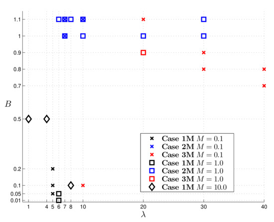
Figure 12. The position of the points in parameter space indicates which case occurs. The picture shows only the couples $(\lambda ,B)$ for given M of Table 2.

We remark that the presence of the external magnetic field complicates the motion and the search for the plug regions because we have to solve a system and no longer an equation in order to get $C_0$, $y_0$, $y_1$, $y_2$, $y_3$. Actually $t_{12}$ depends on the induced magnetic field which is unknown and so we cannot obtain the plug regions in terms of the material parameters alone. Moreover, Table 2 shows that more M increases the more difficult it is to get cases 2M and 3M; this is not surprising also bearing in mind that the presence of the external magnetic field tends to prevent the reverse flow phenomenon [5,15].

The behaviour of the velocity in the three cases is showed in Figure 13. The Case 3M shows the reverse flow phenomenon with $\lambda$ very large ($\lambda \sim 80$) due to the presence of the magnetic field.

Figure 13. Profile of the velocity in the three cases.

For the sake of brevity, we just show how the velocity and the induced magnetic field are influenced by the three parameters in Case 1M (see Figure 14 and Figure 15). We notice that the influence of B and $\lambda$ on the velocity is analogous to the case in which the magnetic field is not present. As the Hartmann number M increases the velocity decreases and the plug region increases its thickness with M. As far as the induced magnetic field is concerned, the trend is similar to the Newtonian case. In particular h is a decreasing function of B and is a increasing function of $\lambda$, while the modulus of the induced magnetic field is not monotone when the Hartmann number changes (as showed in [14]).

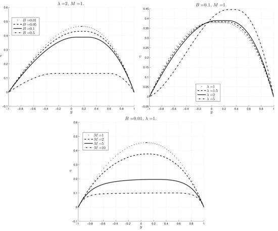
Figure 14. Case 1M: profile of the velocity.

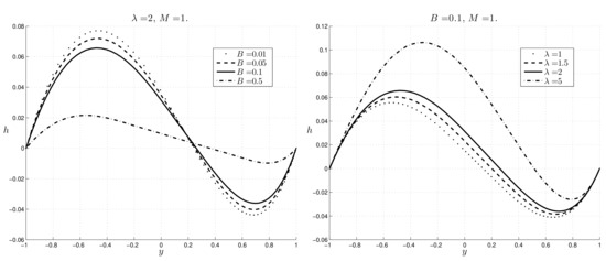
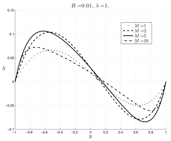
Figure 15. Case 1M: profile of the induced magnetic field.

Figure 16 shows the boundaries of the plug regions: we have that $y_1$ decreases with B and increases with $\lambda$, while $y_2$ increases with B and $\lambda$, as in the absence of the external magnetic field. When M increases, $y_1$ and $y_2$ increase.

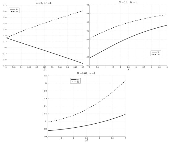
Figure 16. Case 1M: plug boundaries ($y_1$, $y_2$).

6. Conclusions

The problem of the steady mixed convection of a Bingham fluid in a vertical channel in the absence and in the presence of an external uniform magnetic field ${\mathbf{H}}_0$ is studied in the details obtaining the analytical solution: the velocity, the induced magnetic field and the temperature. The plug regions are determined: they depend on the Bingham number B, on the buoyancy parameter $\lambda$ and on the Hartmann number M. Moreover, the velocity decreases and the thickness of the plug region increases as the magnetic field increases. Due to the presence of the buoyancy forces, the reverse flow may occur, as it happens in the case of a Newtonian fluid, but now the magnitude of $\lambda$ must be very large ($\lambda >6$ in the absence of ${\mathbf{H}}_0$, $\lambda \ge 10$ in the presence of ${\mathbf{H}}_0$). Finally, the magnetic field tends to prevent the reverse flow phenomenon as for a Newtonian fluid.

References

- Borrelli, A.; Giantesio, G.; Patria, M.C. Exact solutions in MHD natural convection flow of a Bingham fluid in a vertical channel. submitted.
- Bingham, E.C. Fluidity and Plasticity; McGraw-Hill Book Company, Inc.: New York, NY, USA, 1922. [Google Scholar]
- Obando, B.; Takahashi, T. Existence of weak solutions for a Bingham fluid-rigid body system. Ann. l’Institut Henri Poincaré 2019, 36, 1281–1309. [Google Scholar] [CrossRef]
- Nouar, C.; Frigaard, I.A. Nonlinear stability of Poiseuille flow of a Bingham fluid; theoretical results and comparison with phenomenological criteria. J. Non Newt. Fluid Mech. 2001, 100, 127–149. [Google Scholar] [CrossRef]
- Borrelli, A.; Patria, M.C.; Piras, E. Spatial decay estimate in the problem of entry flow for a Bingham fluid filling a pipe. Mat. Comp. Model. 2004, 40, 23–42. [Google Scholar] [CrossRef]
- Chen, Y.L.; Zhu, K.Q. Couette-Poiseuille flow of Bingham fluids between two porous parallel plates with slip conditions. J. Non Newt. Fluid Mech. 2008, 153, 1–11. [Google Scholar] [CrossRef]
- Barletta, A.; Mayari, E. Buoyant Couette-Bingham flow between vertical parallel plates. Int. J. Therm. Sci. 2008, 47, 811–819. [Google Scholar] [CrossRef]
- Frigaard, I.A.; Karimfazli, I. Natural convection flows of a Bingham fluid in a long vertical channel. J. Non Newt. Fluid Mech. 2013, 201, 39–55. [Google Scholar]
- Bayazitoglu, Y.; Palay, P.R.; Cenocky, P. Laminar Bingham fluid flow between vertical parallel plates. Int. J. Thermal Sci. 2007, 46, 349–357. [Google Scholar] [CrossRef]
- Rees, D.A.S.; Bassom, A.P. The Effect of Internal and External Heating on the Free Convective Flow of a Bingham Fluid in a Vertical Porous Channel. Fluids 2019, 4, 95. [Google Scholar] [CrossRef]
- Patel, N.; Ingham, D.B. Analytic solutions for the mixed convection flow of non-Newtonian fluids in parallel plate ducts. Int. Comm. Heat Mass Transf. 1994, 21, 75–84. [Google Scholar] [CrossRef]
- Aung, W.; Worku, G. Developing flow and flow reversal in a vertical channel with asymmetric wall temperature. ASME J. Heat Transf. 1986, 108, 299–304. [Google Scholar] [CrossRef]
- Aung, W.; Worku, G. Theory of fully developed combined convection including flow reversal. ASME J. Heat Transf. 1986, 108, 485–488. [Google Scholar] [CrossRef]
- Borrelli, A.; Giantesio, G.; Patria, M.C. Magnetoconvection of a micropolar fluid in a vertical channel. Int. J. Heat Mass Transf. 2015, 80, 614–625. [Google Scholar] [CrossRef]
- Borrelli, A.; Giantesio, G.; Patria, M.C. Reverse Flow in Magnetoconvection of Two Immiscible Fluids in a Vertical Channel. J. Fluid Eng. 2017, 139, 101203–101216. [Google Scholar] [CrossRef]
- Misra, J.C.; Adhikary, S.D. Flow of Bingham fluid in a porous bed under the action of a magnetic field: Application to magneto-hemorheology. Eng. Sci. Tech. Int. J. 2017, 20, 973–981. [Google Scholar] [CrossRef][Green Version]
- Pourjafar, M.; Malmir, F.; Bazargan, S.; Sadeghy, K. Magnetohydrodynamic flow of Bingham fluids in a plane channel: A theoretical study. J. Non-Newton. Fluid Mech. 2019, 264, 1–18. [Google Scholar] [CrossRef]
- Vishnyakov, V.I.; Vishnyakova, S.M.; Druzhinin, P.V.; Pokrovskii, L.D. Unsteady flow of an electrically conducting Bingham fluid in a plane magntohydrodynamic channel. J. Appl. Mech. Tech. Phys. 2019, 60, 432–437. [Google Scholar] [CrossRef]
- Barletta, A. Laminar mixed convection with viscous dissipation in a vertical channel. Int. J. Heat Mass Transf. 1998, 41, 3501–3513. [Google Scholar] [CrossRef]
Publisher’s Note: MDPI stays neutral with regard to jurisdictional claims in published maps and institutional affiliations. |
© 2021 by the authors. Licensee MDPI, Basel, Switzerland. This article is an open access article distributed under the terms and conditions of the Creative Commons Attribution (CC BY) license (https://creativecommons.org/licenses/by/4.0/).