Abstract
In the present work, we study the normal shock wave flow problem using a combination of the OBurnett equations and the Holian conjecture. The numerical results of the OBurnett equations for normal shocks established several fundamental aspects of the equations such as the thermodynamic consistency of the equations, and the existence of the heteroclinic trajectory and smooth shock structures at all Mach numbers. The shock profiles for the hydrodynamic field variables were found to be in quantitative agreement with the direct simulation Monte Carlo (DSMC) results in the upstream region, whereas further improvement was desirable in the downstream region of the shock. For the discrepancy in the downstream region, we conjecture that the viscosity–temperature relation () needs to be modified in order to achieve increased dissipation and thereby achieve better agreement with the benchmark results in the downstream region. In this respect, we examine the Holian conjecture (HC), wherein transport coefficients (absolute viscosity and thermal conductivity) are evaluated using the temperature in the direction of shock propagation rather than the average temperature. The results of the modified theory (OBurnett + HC) are compared against the benchmark results and we find that the modified theory improves upon the OBurnett results, especially in the case of the heat flux shock profile. We find that the accuracy gain is marginal at lower Mach numbers, while the shock profiles are described better using the modified theory for the case of strong shocks.
1. Introduction
In the continuum regime for vanishing Knudsen numbers (), the linear constitutive laws (Newton’s law of viscosity and Fourier’s law of heat conduction) employed in the Navier-Stokes equations are sufficient to discern the flow physics. However, as we start moving into the slip regime () and the transition regime () by virtue of the reduction in the characteristic length scale (L) or increase in the mean free path (), these linear constitutive laws are shown to be inaccurate [1,2,3,4,5]. Several non-equilibrium flow phenomena [6,7,8] start arising in the flow that cannot be described using the Navier-Stokes equations. For such flows, it becomes necessary to employ particle methods such as the direct simulation Monte Carlo (DSMC) technique [9,10] or formulate higher-order continuum theories starting from the Boltzmann kinetic equation, for example, conventional Burnett equations [11,12], Grad 13 moment equations [13,14], Onsager-Burnett equations [15], and Onsager 13 moment equations [16]. These higher-order continuum theories have shown promise in modeling simple flow problems such as force-driven plane Poiseuille flow [17,18], shear-driven Couette flow [19,20], and the recently proposed Grad’s second problem [21,22]. However, the fundamental limitations of some of these theories, such as conventional Burnett equations and Grad moment equations, have also been exposed for shock waves, which have somewhat restricted the mainstream adoption of these higher-order continuum theories.
For the shock wave flow problem, the Mach number and Knudsen number are two important dimensionless numbers that characterize the flow problem. The Mach number is greater than unity and is defined as the ratio of the speed of the shock to the adiabatic sound speed. The Knudsen number is of the order of unity and falls well within the transition regime (). With such a high degree of non-equilibrium across the shock, the Navier-Stokes equations fail to quantitatively agree with the benchmark results for Mach numbers () greater than [23,24,25,26,27,28]. The solution to the same problem within the higher-order continuum framework was also not successful. For example, the conventional Burnett equations become invalidated for owing to the unstable nature of the equations, possible violation of the second law of thermodynamics, and the non-existence of the heteroclinic trajectory [25,29,30,31]. In case of the hyperbolic Grad 13 moment equations, discontinuity (sub-shocks) is observed in the shock profiles for [4,32]. Furthermor, the Grad distribution function assumes unphysical negative values for , invalidating the moment equations at higher Mach numbers [33]. Only recently [34], we showed that the OBurnett equations based on the Onsager-consistent approach do not suffer from these limitations and, at the same time, provide significant improvement over the results of Navier-Stokes equations for all Mach numbers. Without tweaking the equations in any way, the equations accurately resolved the upstream region of the shock, whereas some discrepancy was observed in the downstream region. In the present work, we modified the OBurnett equations by incorporating the Holian conjecture (HC) [35,36,37] in order to achieve quantitative agreement in the downstream region. In the present work, the modified theory (OBurnett + HC) was tested for a wide Mach number range including the case of a very strong shock (), and the results were benchmarked against the DSMC/non-equilibrium molecular dynamics (NEMD) results for a dilute gas system composed of hard-sphere molecules.
The remainder of this paper is organized as follows: The OBurnett equations are introduced in Section 2, with a brief introduction to the Onsager-consistent approach. In Section 3, the significance and superiority of the OBurnett equations over other higher-order continuum theories are highlighted. The problem definition for the normal shock wave flow problem is introduced in Section 4, and the reduced form of the equations based on the modified theory (OBurnett + HC) is dscribed in Section 5. The results are presented in Section 6, followed by the important conclusions in Section 7.
2. OBurnett Equations
The Onsager-Burnett (OBurnett) equations belong to a class of higher-order continuum transport equations that form a super-set of Navier-Stokes equations. In the derivation of these equations, the Onsager-consistent approach forms the basis that is completely independent of the Chapman-Enskog approach or the Grad moment method. In the Onsager-consistent approach, we ignore the traditional phenomenological approach of deriving continuum theories; rather, we start with the fundamental Boltzmann equation from kinetic theory, which is given as:
where is the single particle distribution function, which represents the solution of the Boltzmann equation; is th location of a particle in physical space; is the molecular velocity; t is the time variable; is the external force per unit mass acting on the molecules; and represents the collision integral.
The transition from microscopic to macroscopic dynamics can be achieved by taking the appropriate moments of the Boltzmann equation. The macroscopic properties of interest, such as density, bulk velocity, and temperature, are related to the distribution function as
where n is the number density of the molecules, m is the molecular mass, and is the Boltzmann constant.
Multiplying the Boltzmann equation by and then integrating over the velocity space, the basic conservation laws of mass, momentum, and energy can be obtained as
where is the mass density, is the bulk velocity vector, p is the thermodynamic pressure, is the heat flux vector, is the stress tensor, is the external body force per unit mass, () is the internal energy, and T is the absolute temperature.
It is easily recognized that the above system of equations is not closed as we have 5 equations and 13 unknowns. To obtain a closed set of equations, we need to substitute the constitutive relations for the stress tensor and the heat flux vector in terms of the primary variables and their gradients. In the traditional phenomenological approach employed while deriving the Navier-Stokes equations, the necessary closure is obtained by using Newton’s law of viscosity and Fourier’s law of heat conduction. However, in the kinetic approach, we evaluate the stress tensor and the heat flux vector as
Note that C is peculiar velocity given as and the angular bracket denotes the symmetric and trace-free part of the tensor, given as .
Expressions for the stress tensor (Equation (8)) and the heat flux vector (Equation (9)) can only be evaluated once we know the form of the distribution function, i.e., we need to solve the Boltzmann equation for the distribution function. The Chapman-Enskog approach, the Grad moment method, and the Onsager-consistent approach focus on obtaining the form of the distribution function, and all these approaches are independent of one another. In the Onsager-consistent approach [15], the distribution function is represented in terms of the thermodynamic forces and fluxes [16,38,39] as
where represents the Maxwell–Boltzmann distribution function and the subscript O in signifies that the distribution function is consistent with Onsager’s reciprocity principle. When the series is truncated until the Maxwell–Boltzmann distribution, we can obtain the inviscid Euler equations. Taking into account the first-order correction terms, the Navier-Stokes equations can be obtained, which are first-order accurate for Knudsen number. As we extend one step further by considering the second-order correction terms, the OBurnett equations can be obtained, which form a super-set of the Navier-Stokes equations and are second-order accurate for Knudsen number.
In the Onsager-consistent approach, the formulation of the distribution function is performed carefully so that it is consistent with Onsager’s symmetry principle [40,41] and the H-theorem. As these important principles are satisfied at the level of the distribution function, we ultimately obtain thermodynamically consistent theory at the macroscopic level. Th Onsager-consistent distribution function also satisfies the linearized Boltzmann equation and the collision invariance property. This particular form of the distribution function is then utilized to derive the OBurnett [15] (Burnett-like) and O13 [16] (Grad-like) equations.
Substituting the expression for the Onsager-consistent distribution function (Equation (10)) in Equations (8) and (9), the OBurnett constitutive relations for the stress tensor and the heat flux vector can be obtained as
where u, v, and w are the x, y, and z components of the bulk velocity vector, respectively; is the absolute viscosity; k is the thermal conductivity of the gas; and is the specific heat ratio. The expressions for and g are given as
The coefficients, , , , and , with numerical subscripts, are functions of the type of gas and the interaction potential between the molecules. The constants appearing in front of the derivatives of flow field variables are
To evaluate the Burnett contribution for other components of the stress tensor and heat flux vector, we apply a suitable change in variables in an appropriate base equation as given in Table 1.

Table 1.
Base equation and change in variables to be followed while evaluating the Burnett-order contribution for other components of the stress tensor and heat flux vector.
3. Significance of the OBurnett Equations
The conventional Burnett equations, as is now well-known [31,39,42], are unstable, known to violate the second law of thermodynamics, and require additional boundary conditions for their complete solution, which are generally unknown. As such, the theory is far from complete and cannot be applied to complex boundary value problems. All these limitations associated with the conventional Burnett equations do not arise in the OBurnett equations. With respect to the boundary conditions part, the OBurnett equations require the same number of boundary conditions as the Navier-Stokes equations. This is evident when we notice the absence of second- and higher-order derivatives of velocity and temperature in the OBurnett constitutive relations. Stability is another important aspect wherein the OBurnett equations score above the conventional Burnett equations. The OBurnett equations are unconditionally stable and, hence, accurate solutions can be obtained on finer grids, which is not possible in the case of conventional Burnett equations. Hence, it is safe to say that the OBurnett equations form a complete theory and can serve as a monolithic solver for simulating flows starting from the continuum regime to the transition regime without any restrictions.
The accuracy of the OBurnett equations in describing non-equilibrium flow phenomena was successfully demonstrated in the force-driven plane compressible flow problem [18]. The equations were shown to capture the non-constant pressure profile, the tangential heat flux, and the presence of the normal stresses, in agreement with the DSMC results. After this initial success, the equations were applied to the shock wave flow problem, which is regarded as the most stringent test case for higher-order continuum theories [34,43]. This flow problem helped to establish several fundamental aspects of the OBurnett equations by providing strong evidence for the following:
- 1.
- Smooth shock structures at all Mach numbers;
- 2.
- Existence of the heteroclinic trajectory (a curve connecting the upstream and downstream equilibrium states);
- 3.
- Positive entropy generation at all Mach numbers, implying the thermodynamic consistency of the equations.
It is important to highlight that neither the conventional Burnett equations nor the Grad 13 moment equations satisfy all these claims. For example, the heteroclinic trajectory does not exist for the conventional Burnett equations for and the equations predict negative entropy generation in the upstream region of the shock [25,30,43]. In the case of moment equations, since the equations are hyperbolic, the issue of subshocks arise and we cannot obtain smooth shock structures for [2,4,32,33]. This properties help to establish the superiority of the OBurnett equations over the conventional Burnett equations and the Grad moment equations.
While describing the shock structures for the hydrodynamic field variables using the OBurnett equations [34,43], the equations provide significant improvement over the results of the Navier-Stokes equations for a wide range of Mach numbers. Further comparison with the benchmark data (DSMC/NEMD results) revealed that the agreement is quantitative in the upstream region, whereas further improvement is desirable in the downstream region. This result was a bit surprising since the more rarefied upstream region is supposedly more difficult to resolve than the downstream region. In order to explain this behavior, we conjecture that the relation between the viscosity and the absolute temperature () is insufficient to capture the flow physics in the high-temperature, downstream region. To be more specific, the dissipation needs to be increased in the downstream region either by enhancing the viscosity index, as in [27,28], or by employing the Holian conjecture [35,36,37]. In the present work, we apply the Holian conjecture in the OBurnett equations and aim to verify whether the modified theory reasonably agrees with the benchmark data in the downstream region of the shock.
4. Problem Definition
A typical normal shock wave consists of two equilibrium states, namely the upstream state before the shock and the downstream state after the shock, as shown in Figure 1. The shock wave propagates with a constant velocity; hence, modeling the problem in the shock wave reference frame removes the time dependency in the governing equations. This simplification reduces the complexity of the problem, and an important aspect of the time of shock formation does not apply. Accordingly, all the hydrodynamic variables are now functions of the x coordinate only; hence, the problem can be modeled in a one-dimensional framework. As such, the velocity vector (), the stress tensor (), and the heat flux vector () have only their x components, which are u, , and , respectively.
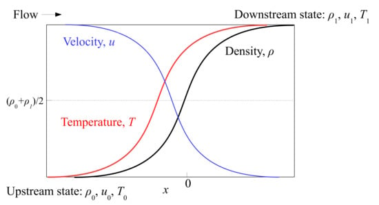
Figure 1.
Schematic of the internal structure of a one-dimensional normal shock wave.
The upstream state is characterized by supersonic velocity (), whereas the velocity at the downstream state is subsonic (). The thermodynamic variables, density and temperature, rise sharply from the upstream state (, ) to the downstream state (, ) across the narrow region of the shock. These strong gradients of the field variables induces dissipative effects inside the shock region leading to the formation of a strong non-equilibrium region across the narrow width of the shock. Accordingly, the mass, momentum, and energy conservation equations (Equations (5)–(7)) can be readily obtained as
where the normal stress and x component of the heat flux vector are represented by and q, respectively. The thermodynamic pressure p appearing in the momentum and energy equation can be replaced using ideal gas equation as
Furthermore, for a dilute, monatomic gas system, the internal energy of a monatomic gas without internal degrees of freedom is given as
Substituting for p and , the conservation Equations (15)–(17) can be written in a more convenient form as
Noting that the stresses and heat fluxes are absent before and after the shock ( and ) owing to the zero gradients of the field variables, the Rankine-Hugoniot conditions can be obtained by performing integration between the upstream and downstream equilibrium states as
where we use Equation (23) to obtain Equation (25).
To obtain the variation in the hydrodynamic field variables across the shock, we need to carry out the integration between the upstream state and any point inside the shock as
Note that the above equations are not in a closed form, and we need to substitute the constitutive relations for the normal stress and the heat flux. The OBurnett constitutive relations for the normal shock wave flow problem can be obtained as
The space coordinate and other field variables are non-dimensionalized, as in [29,36]
The quantities l and are different and related to each other as . Note that is defined at the upstream point for the case of hard-sphere molecules, and the transport coefficients are proportional to square root of temperature as [12]
where is the particle diameter and the coefficients and are taken as 1.
By substituting the OBurnett constitutive relations for normal stress (Equation (29)) and heat flux (Equation (30)), the closed form of the momentum (27) and energy (28) equations can be obtained. The final non-dimensionalized form of the reduced OBurnett equations was derived in our earlier work (see Equations (28) and (29) in [34]). Without repeating the mathematical details, the final equations read as
where , where Pr is the Prandtl number, which is for monatomic gases. The relevant OBurnett coefficients for the case of hard-sphere molecules () are obtained as
The Rankine-Hugoniot conditions in the non-dimensionalized form can be obtained as
5. Modified Theory: OBurnett + HC
In this section, we combine OBurnett theory and the Holian conjecture and present the reduced form of the equations for the modified theory. The main idea of the Holian conjecture [35,36] is to modify the viscosity–temperature relation () by replacing the average temperature (T) with the component of temperature in the direction of the shock propagation (). The average temperature is related to the directional temperatures as
For a monatomic gas, the temperature component can be extracted from the normal component of pressure tensor as
Note that the pressure tensor is related to the stress tensor as , so that the relation can be obtained.
The temperature in the direction of the shock propagation () is always greater than the average temperature (T). By replacing T with in the viscosity-temperature relation, we are essentially increasing the viscosity across the shock region. This results in increased dissipation, thereby broadening the shock profiles for the case of strong shocks. This modification when applied to the Navier-Stokes equations provides reasonable agreement with the NEMD results for strong shocks (), as shown in [36].
Here, we apply the Holian conjecture in OBurnett theory by correcting only the Navier-Stokes-order terms of the stress tensor and the heat flux vector. We do not attempt to correct the Burnett-order terms since the magnitude of these terms will be small compared to that of the Navier-Stokes terms and most of the Burnett-order terms are actually independent of temperature, as also noted in [37]. Following this procedure, it can be shown that the term appearing in the underlined terms of Equations (32) and (33) needs to be replaced with , and the expression for is given as [35,36,44],
The final form of the system of the ordinary differential equations for the modified theory (OBurnett + HC) then assumes the form
The Rankine-Hugoniot boundary conditions given in Equation (35) remain same for the modified theory. The system of Equations (39) and (40) is tackled as an initial value problem as performed in the literature [25,29,36,45]. The adopted numerical procedure is the same as followed in our earlier works [34,43]. The MATLAB solver ode15i of order 5 was selected to solve the implicit system of ordinary differential equations with the relative and absolute errors set to and , respectively. Once we obtain the solution for velocity and temperature, other shock profiles for density, normal stress, and heat flux can be readily obtained as
The results of the shock profiles for three Mach numbers ( = 3, 9, and 134) are presented in the ensuing sections.
6. Results
In this section, the variation in the conserved variables (, , and ) and the non-conserved variable () across the narrow region of the shock, as obtained by combination of the OBurnett equations and the Holian conjecture, is compared with the benchmark DSMC results. To generate the DSMC results, Bird’s DSMC code [9] for the normal shock wave flow problem was implemented; details are provided in our earlier work [43]. By employing the combination of the OBurnett equations and the Holian conjecture, we first verified the thermodynamic consistency of the modified theory and the existence of the heteroclinic trajectory. The results indicate that the modified theory satisfies all these fundamental aspects, similar to the OBurnett equations [34].
The shock profiles for the velocity, density, temperature, and the heat flux for two Mach numbers, 3 and 9, are shown in Figure 2 and Figure 3. The effect of the increased dissipation that is achieved by employing the Holian conjecture is not that significant for the conserved variables, as is evident from the velocity (Figure 2a and Figure 3a), density (Figure 2b and Figure 3b), and temperature (Figure 2c and Figure 3c) shock profiles. The modified theory marginally improves upon the results of the OBurnett equations in the downstream region due to increased dissipation. However, the same cannot be said for the upstream region, where the results of the modified theory and the OBurnett equations are almost indistinguishable. For the heat flux (Figure 2d and Figure 3d), the modified theory accurately captures the peak of the heat flux while improving upon the results of the OBurnett equations. An interesting phenomenon of temperature overshoot is observed in the downstream region of the shock where the temperature of the gas molecules exceeds that downstream. This behavior is confirmed by the experiments as well as the DSMC method and is probably due to the delayed relaxation of the transversal kinetic energy of the gas molecules. Although higher-order terms are added in the constitutive relation of heat flux vector in OBurnett theory, we observe a monotonous rise in the temperature across the shock as per the modified theory.
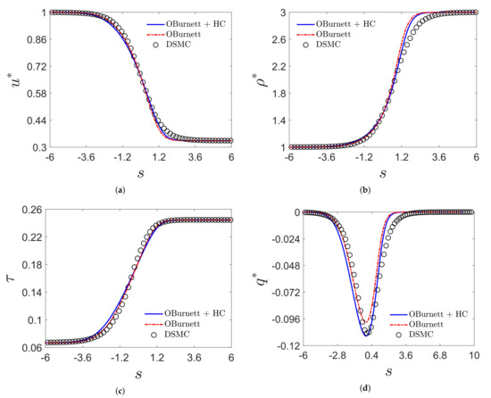
Figure 2.
Variation in hydrodynamics field (a) velocity, (b) density, (c) temperature, and (d) heat flux across the shock for .
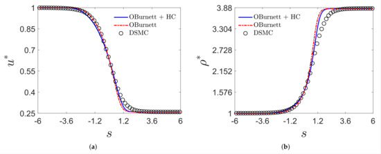
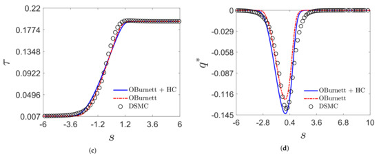
Figure 3.
Variation in hydrodynamics field (a) velocity, (b) density, (c) temperature, and (d) heat flux across the shock for .
The case of a very strong shock with is also studied using the modified theory (Figure 4) and the results are compared against the non-equilibrium molecular dynamics (NEMD) results, as obtained by Salamons and Mareschal [26]. For the velocity (Figure 4a) and the density (Figure 4b) profiles, we observe that the modified theory provides significant improvement in the downstream region compared with the results of the OBurnett equations. However, the temperature profile is described much better by the OBurnett equations than the modified theory, both in the upstream and the downstream regions. With respect to the heat flux profile (Figure 4d), the results of the modified theory are in good agreement with those of the NEMD with substantial improvement achieved compared to the OBurnett results.
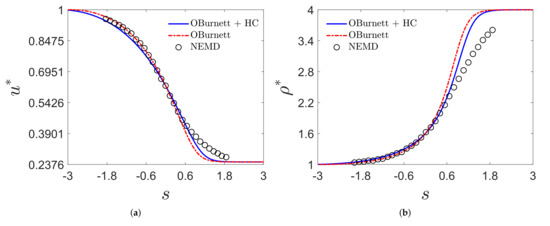
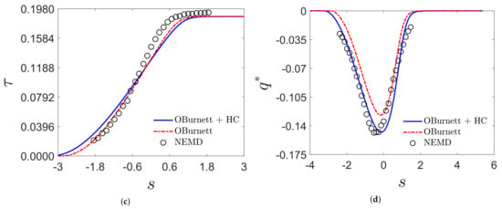
Figure 4.
Variation in hydrodynamics field (a) velocity, (b) density, (c) temperature, and (d) heat flux across the shock for . Non-equilibrium molecular dynamics (NEMD) results were obtained from [26].
For all the three cases studied here ( = 3, 9, and 134), we observe that the shock thickness increases only slightly with the Mach number. This observation is consistent with the experimental and the DSMC results in the literature [46,47], where it is shown that the for higher Mach numbers, the shock thickness based on density profiles increases only slightly with Mach number.
In summary, the Holian conjecture when applied to OBurnett theory, a modified theory, performs well for the case of a very strong shock. However, for weak shocks, the modified theory provides marginal improvement over the results of the OBurnett equations. Hence, our hypothesis that the modified theory will be able to resolve the downstream region well only for the case of strong shocks. This also implies that the applicability of the Holian conjecture is only for strong shocks, as also noted in the works of [37,48].
7. Conclusions
In the present work, we proposed a modified theory by combining the OBurnett equations and the Holian conjecture (OBurnett + HC) to model the normal shock waves for a dilute gas system of hard-sphere molecules. Rather than using the average temperature, the longitudinal temperature in the direction of the shock propagation was used in the evaluation of the transport coefficients. The sole aim of this modification was to achieve increased dissipation in the hot region of the shock and thereby obtain better quantitative agreement with the benchmark results than the previously obtained OBurnett results. The modified theory still formed an entropic consistent system, a clear heteroclinic trajectory existed, and smooth shock structures were obtained at all Mach numbers, similar to OBurnett theory. For two Mach numbers tested ( = 3 and 9), the modified theory improved upon the OBurnett results for the heat flux shock profiles. However, the accuracy gain for the other hydrodynamic fields (, , and ) was only marginal. The results for the case of a very strong shock () were significantly improved using the modified theory, with excellent agreement observed for the heat flux profile. These results suggest that accounting for the Holian conjecture in the OBurnett equations works better for the case of strong shocks, whereas the original OBurnett theory seems to be a better choice for modeling weak shocks.
Author Contributions
Conceptualization and methodology, R.S.J. and A.A.; formal analysis, investigation, and writing—original draft preparation, R.S.J.; writing—review and editing, A.A.; supervision, A.A.; project administration and funding acquisition, A.A. All authors have read and agreed to the published version of the manuscript.
Funding
This work was performed as part of the Department of Atomic Energy Science Research Council Outstanding Investigator Award (21/01/2015-BRNS/35038).
Institutional Review Board Statement
Not applicable.
Informed Consent Statement
Not applicable.
Conflicts of Interest
The authors declare no conflict of interest.
Abbreviations
The following abbreviations are used in this manuscript:
| OBurnett | Onsager-Burnett |
| HC | Holian Conjecture |
| DSMC | Direct Simulation Monte Carlo |
| NEMD | Non-equilibrium Molecular Dynamics |
References
- Gad-el Hak, M. The fluid mechanics of microdevices—The Freeman scholar lecture. J. Fluids Eng. 1999, 121, 5–33. [Google Scholar] [CrossRef]
- Torrilhon, M. Modeling Nonequilibrium Gas Flow Based on Moment Equations. Annu. Rev. Fluid Mech. 2016, 48, 429–458. [Google Scholar] [CrossRef]
- Uribe, F.; Garcia, A. Burnett description for plane Poiseuille flow. Phys. Rev. E 1999, 60, 4063–4078. [Google Scholar] [CrossRef] [PubMed] [Green Version]
- Grad, H. The profile of a steady plane shock wave. Commun. Pure Appl. Math. 1952, 5, 257–300. [Google Scholar] [CrossRef]
- Myong, R. Theoretical description of the gaseous Knudsen layer in Couette flow based on the second-order constitutive and slip-jump models. Phys. Fluids 2016, 28, 012002. [Google Scholar] [CrossRef]
- Balaj, M.; Roohi, E.; Mohammadzadeh, A. Regulation of anti-Fourier heat transfer for non-equilibrium gas flows through micro/nanochannels. Int. J. Therm. Sci. 2017, 118, 24–39. [Google Scholar] [CrossRef]
- Mohammadzadeh, A.; Rana, A.S.; Struchtrup, H. Thermal stress vs. thermal transpiration: A competition in thermally driven cavity flows. Phys. Fluids 2015, 27, 112001. [Google Scholar] [CrossRef] [Green Version]
- Hemadri, V.; Biradar, G.S.; Shah, N.; Garg, R.; Bhandarkar, U.V.; Agrawal, A. Experimental study of heat transfer in rarefied gas flow in a circular tube with constant wall temperature. Exp. Therm. Fluid Sci. 2018, 93, 326–333. [Google Scholar] [CrossRef]
- Bird, G.A.; Brady, J. Molecular Gas Dynamics and the Direct Simulation of Gas Flows; Clarendon press Oxford: Oxford, UK, 1994; Volume 42. [Google Scholar]
- Bird, G. The DSMC Method; CreateSpace Independent Publishing Platform: Scotts Valley, CA, USA, 2013. [Google Scholar]
- Burnett, D. The distribution of molecular velocities and the mean motion in a non-uniform gas. Proc. Lond. Math. Soc. 1936, 2, 382–435. [Google Scholar] [CrossRef]
- Chapman, S.; Cowling, T.G. The Mathematical Theory of Non-Uniform Gases: An Account of the Kinetic Theory of Viscosity, Thermal Conduction and Diffusion in Gases; Cambridge University Press: Cambridge, UK, 1970. [Google Scholar]
- Grad, H. On the kinetic theory of rarefied gases. Commun. Pure Appl. Math. 1949, 2, 331–407. [Google Scholar] [CrossRef]
- Grad, H. Principles of the Kinetic Theory of Gases. In Thermodynamik der Gase/Thermodynamics of Gases; Springer: Berlin/Heidelberg, Germany, 1958; pp. 205–294. [Google Scholar]
- Singh, N.; Jadhav, R.S.; Agrawal, A. Derivation of stable Burnett equations for rarefied gas flows. Phys. Rev. E 2017, 96, 013106. [Google Scholar] [CrossRef]
- Singh, N.; Agrawal, A. Onsager’s-principle-consistent 13-moment transport equations. Phys. Rev. E 2016, 93, 063111. [Google Scholar] [CrossRef] [PubMed]
- Tij, M.; Santos, A. Perturbation analysis of a stationary nonequilibrium flow generated by an external force. J. Stat. Phys. 1994, 76, 1399–1414. [Google Scholar] [CrossRef]
- Jadhav, R.S.; Singh, N.; Agrawal, A. Force-driven compressible plane Poiseuille flow by Onsager-Burnett equations. Phys. Fluids 2017, 29, 102002. [Google Scholar] [CrossRef]
- Lockerby, D.A.; Reese, J.M. High-resolution Burnett simulations of micro Couette flow and heat transfer. J. Comput. Phys. 2003, 188, 333–347. [Google Scholar] [CrossRef]
- Singh, N.; Gavasane, A.; Agrawal, A. Analytical solution of plane Couette flow in the transition regime and comparison with Direct Simulation Monte Carlo data. Comput. Fluids 2014, 97, 177–187. [Google Scholar] [CrossRef]
- Jadhav, R.S.; Agrawal, A. Grad’s second problem and its solution within the framework of Burnett hydrodynamics. J. Heat Transf. 2020, 142, 102105. [Google Scholar] [CrossRef]
- Jadhav, R.S.; Agrawal, A. Evaluation of Grad’s Second Problem Using Different Higher Order Continuum Theories. J. Heat Transf. 2021, 143, 012102. [Google Scholar] [CrossRef]
- Becker, R. Impact Waves and Detonation; Zeitschrift für Physik Transtation, N.A.C.A.-T.M. No. 505 (1929); Springer: Berlin/Heidelberg, Germany, 1929; Volume 8, pp. 321–362. [Google Scholar]
- Thomas, L. Note on Becker’s theory of the shock front. J. Chem. Phys. 1944, 12, 449–453. [Google Scholar] [CrossRef]
- Uribe, F.; Velasco, R.; Garcia-Colin, L.; Diaz-Herrera, E. Shock wave profiles in the Burnett approximation. Phys. Rev. E 2000, 62, 6648. [Google Scholar] [CrossRef] [PubMed]
- Salomons, E.; Mareschal, M. Usefulness of the Burnett description of strong shock waves. Phys. Rev. Lett. 1992, 69, 269. [Google Scholar] [CrossRef] [PubMed]
- Greenshields, C.J.; Reese, J.M. The structure of shock waves as a test of Brenner’s modifications to the Navier–Stokes equations. J. Fluid Mech. 2007, 580, 407–429. [Google Scholar] [CrossRef] [Green Version]
- Uribe, F.; Velasco, R. Shock-wave structure based on the Navier-Stokes-Fourier equations. Phys. Rev. E 2018, 97, 043117. [Google Scholar] [CrossRef] [PubMed]
- Uribe, F.J.; Velasco, R.M.; García-Colín, L.S. Burnett Description of Strong Shock Waves. Phys. Rev. Lett. 1998, 81, 2044–2047. [Google Scholar] [CrossRef]
- Comeaux, K.A.; Chapman, D.R.; MacCormack, R.W. An analysis of the Burnett equations based on the second law of thermodynamics. In Proceedings of the 33rd Aerospace Sciences Meeting and Exhibit, Reno, NV, USA, 9–12 January 1995; p. 415. [Google Scholar]
- Garcia-Colin, L.; Velasco, R.; Uribe, F. Beyond the Navier-Stokes equations: Burnett hydrodynamics. Phys. Rep. 2008, 465, 149–189. [Google Scholar] [CrossRef]
- Weiss, W. Continuous shock structure in extended thermodynamics. Phys. Rev. E 1995, 52, R5760–R5763. [Google Scholar] [CrossRef] [PubMed]
- Torrilhon, M.; Struchtrup, H. Regularized 13-moment equations: Shock structure calculations and comparison to Burnett models. J. Fluid Mech. 2004, 513, 171–198. [Google Scholar] [CrossRef] [Green Version]
- Jadhav, R.S.; Agrawal, A. Strong shock as a stringent test for Onsager-Burnett equations. Phys. Rev. E 2020, 102, 063111. [Google Scholar] [CrossRef]
- Holian, B.L. Modeling shock-wave deformation via molecular dynamics. Phys. Rev. A 1988, 37, 2562. [Google Scholar] [CrossRef] [PubMed] [Green Version]
- Holian, B.L.; Patterson, C.; Mareschal, M.; Salomons, E. Modeling shock waves in an ideal gas: Going beyond the Navier-Stokes level. Phys. Rev. E 1993, 47, R24. [Google Scholar] [CrossRef] [PubMed]
- He, Y.; Tang, X.; Pu, Y. Modeling shock waves in an ideal gas: Combining the Burnett approximation and Holian’s conjecture. Phys. Rev. E 2008, 78, 017301. [Google Scholar] [CrossRef] [PubMed]
- Mahendra, A.K.; Singh, R.K. Onsager reciprocity principle for kinetic models and kinetic schemes. arXiv 2013, arXiv:1308.4119. [Google Scholar]
- Agrawal, A.; Kushwaha, H.M.; Jadhav, R.S. Microscale Flow and Heat Transfer: Mathematical Modelling and Flow Physics; Springer: Cham, Switzerland, 2020. [Google Scholar]
- Onsager, L. Reciprocal relations in irreversible processes. I. Phys. Rev. 1931, 37, 405. [Google Scholar] [CrossRef]
- Onsager, L. Reciprocal relations in irreversible processes. II. Phys. Rev. 1931, 38, 2265. [Google Scholar] [CrossRef] [Green Version]
- Struchtrup, H. Macroscopic Transport Equations for Rarefied Gas Flows; Springer: Berlin/Heidelberg, Germany, 2005. [Google Scholar]
- Jadhav, R.S.; Gavasane, A.; Agrawal, A. Improved theory for shock waves using the OBurnett equations. J. Fluid Mech. 2021, 929, A37. [Google Scholar] [CrossRef]
- Holian, B. A History of constitutive modeling via molecular dynamics: Shock waves in fluids and gases. In Proceedings of the EPJ Web of Conferences. EDP Sciences, Poitiers, France, 4–9 July 2010; Volume 10, p. 00002. [Google Scholar]
- Gilbarg, D.; Paolucci, D. The Structure of Shock Waves in the Continuum Theory of Fluids. J. Ration. Mech. Anal. 1953, 2, 617–642. [Google Scholar]
- Alsmeyer, H. Density profiles in argon and nitrogen shock waves measured by the absorption of an electron beam. J. Fluid Mech. 1976, 74, 497–513. [Google Scholar] [CrossRef]
- Solovchuk, M.A.; Sheu, T.W. Prediction of strong-shock structure using the bimodal distribution function. Phys. Rev. E 2011, 83, 026301. [Google Scholar] [CrossRef] [Green Version]
- Velasco, R.; Uribe, F. A study on the Holian conjecture and Linear Irreversible Thermodynamics for shock-wave structure. Wave Motion 2021, 100, 102684. [Google Scholar] [CrossRef]
Publisher’s Note: MDPI stays neutral with regard to jurisdictional claims in published maps and institutional affiliations. |
© 2021 by the authors. Licensee MDPI, Basel, Switzerland. This article is an open access article distributed under the terms and conditions of the Creative Commons Attribution (CC BY) license (https://creativecommons.org/licenses/by/4.0/).