Abstract
Turbulence in the edge plasma of a tokamak is a key actor in the determination of the confinement properties. The divertor configuration seems to be beneficial for confinement, suggesting an effect on turbulence of the particular magnetic geometry introduced by the X-point. Simulations with the 3D fluid turbulence code TOKAM3X are performed here to evaluate the impact of a diverted configuration on turbulence in the edge plasma, in an isothermal framework. The presence of the X-point is found, locally, to affect both the shape of turbulent structures and the amplitude of fluctuations, in qualitative agreement with recent experimental observations. In particular, a quiescent region is found in the divertor scrape-off layer (SOL), close to the separatrix. Globally, a mild transport barrier spontaneously forms in the closed flux surfaces region near the separatrix, differently from simulations in limiter configuration. The effect of turbulence-driven Reynolds stress on the formation of the barrier is found to be weak by dedicated simulations, while turbulence damping around the X-point seems to globally reduce turbulent transport on the whole flux surface. The magnetic shear is thus pointed out as a possible element that contributes to the formation of edge transport barriers.
1. Introduction
In the Deuterium-Tritium phase, ITER is expected to operate in the so-called High-confinement (H) mode. The H-mode regime, in opposition to the Low-confinement mode (L), is characterized by a visible steepening of the profiles of plasma density in the edge region that leads ultimately to a higher plasma pressure at the magnetic axis. This phenomenon is associated with a reduction in turbulent transport, which is the dominant particle and heat transport mechanism in the edge plasma. More specifically, in H-mode conditions, the fluctuation level is strongly reduced in a region of the edge plasma radially localized near the separatrix: this partial turbulence suppression in a localized region is also called “transport barrier”. The transition from L to H-mode is experimentally obtained when the power injected into the plasma exceeds a certain threshold. This power threshold depends on the device characteristics and on the plasma conditions [1]. When the threshold is exceeded, the dynamic system exhibits a bifurcation, the level of fluctuation is drastically reduced, and large relaxation events as edge localized modes (ELMs) are usually observed. The magnetohydrodynamic (MHD) stability and the transport processes in the region affected by the transport barrier are extensively studied in the so-called pedestal physics [2].
Even if the L-H transition is experimentally reproducible, theory cannot yet completely explain this process, making difficult the extrapolation of the existing scaling laws to new devices. Up to now, it seems clear that the suppression of turbulent structures is due to the shear of the plasma velocity in the poloidal direction, which is perpendicular both to the magnetic field and to the direction perpendicular to flux surfaces [3]. However, the cause of this shear is still unclear, and several mechanisms have been pointed out. Indeed, the poloidal velocity derives from the radial profile of the electric field, which tends to balance the radial pressure gradient. Turbulence itself is a potential source of poloidal flows, uniform on a flux surface but with a finite radial wavenumber: these are also called Zonal Flows (ZF). As well-explained in [4], small turbulence scales can, in fact, provide energy to large scale flows in an inverse cascade process, in particular through the mechanism of the Reynolds stress. Therefore small-scale turbulence, which is affected by the shear, contributes to the formation of the shear itself. The problem is complicated by the fact that the characteristics of turbulence depend on the background plasma equilibrium. In fact, the energy available for interchange turbulence depends on the average pressure gradient in the plasma. Also, there are some turbulence saturation mechanisms, which depend on the background gradients [5]. Turbulence is the main transport mechanism and therefore affects, in turn, the global equilibrium. Figure 1 shows schematically the complex interplay between turbulence and the background conditions.

Figure 1.
Sketch of the interplay of physical mechanisms intervening in the formation of transport barriers.
Another element which is affecting turbulence and, in turn, the overall equilibrium, is the magnetic shear, namely the variation of the field line pitch angle in the cross-field direction. In past works, it has been proven that interchange turbulence growth rate is maximum for a certain value of the shear in circular geometries: this can be proven analytically [6] and numerically with linear and non-linear gyrokinetic simulations [7]. Recently, it has been pointed out that the magnetic shear can induce an shear [8]: this synergy further complicates the identification of the primary causes of the build-up of a transport barrier.
The complex problem of the transport barriers calls for an investigation with global turbulence simulations, which are presently able to include all the mentioned aspects of the edge plasma physics. During the years, fluid turbulence codes have addressed the transport barriers problem in various ways. On one hand, transport barriers were forced by regulating some physical parameters in 2D turbulence codes (see e.g., [9,10]), then assessing the effect of barriers on turbulence properties. On the other hand, some anisothermal 2D turbulence codes have reproduced transport barriers by varying the energy source value, in some cases (see e.g., [5,11]) leading to a dynamics in the system behavior coherent with an L-H transition. In 3D global edge turbulence fluid simulations, instead, macroscopic transport barriers have never been highlighted, to our knowledge. An enhancement of radial pressure gradient was observed in Global Braginskii Solver (GBS) simulations in the first open flux surfaces [12], however not associated with a lowering of turbulence levels. It is worth noting that the XGC1 gyrokinetic code [13], simulating an edge plasma with realistic magnetic geometry and physical parameters, has reproduced a bifurcative dynamics associable to the L-H transition. However, in XGC1 simulations, the initial background profiles are artificially imposed, and the system evolves for a small time with respect to the confinement time. Therefore, simulations run on longer time scales are required to better interpret the outcome of these simulations. In this context, 3D fluid turbulence codes can play an important role, giving an insight on global mechanisms as the formation of edge transport barriers.
It is to be noted that the H-mode has been first achieved in the Axially Symmetric Divertor Experiment (ASDEX) [14], when a divertor magnetic configuration was first introduced. Even though several examples of improved confinement exist also in limiter configuration (e.g., [15]), the H-mode is routinely achieved only in divertor configuration. This fact suggests that the particular geometry of the magnetic field in the vicinity of the X-point, can somehow affect the global behavior of turbulence in the edge plasma. In this work, we will exploit the ability of the TOKAM3X code to perform global simulations in divertor configuration [16], to study the effects of the magnetic geometry introduced by the X-point on the turbulence local and global behavior, including the formation of transport barriers. In order to limit the computational cost of simulations we solve, in this work, the isothermal version of the TOKAM3X model. Although the isothermal assumption clearly represents a strong limitation in the description of the edge plasma, first TOKAM3X simulations with the anisothermal model have shown that turbulence nature and statistical properties are qualitatively similar to the isothermal case [17]. Therefore, we expect the general conclusions of this paper to be qualitatively valid also in an anisothermal framework.
In Section 2 we briefly describe TOKAM3X, and the setup of the divertor simulations. In Section 3 we describe the results of the simulations, including the local effect of the X-point on fluctuations shape and amplitude, and the characteristics of the observed transport barrier. We also investigate the physical mechanism underneath the formation of the transport barrier. In Section 4 we isolate the role of the Reynolds stress in driving the poloidal flows. This publication can be seen as complementary of [18], where we described the macroscopic behavior of the background plasma in the same divertor configuration.
2. The TOKAM3X Code
TOKAM3X solves a two-fluid, electrostatic model for electrons and ions. The physical system is obtained by calculating the successive moments of the Boltzmann equation for the two species. The relatively low temperature of the edge plasma, and thus the high collisionality, allows to adopt the so-called Braginskii closure [19]. The large anisotropy of magnetized plasmas is conveniently described by separating the dynamics parallel to the magnetic field to the one perpendicular to it. In particular, equations are drift-reduced, assuming that the characteristic turbulence frequencies are slow compared to the ion cyclotronic frequency. The motion of the fluid in the cross-field direction is given, at the first order, by the drift velocities:
where s denotes the specie, the electric charge of the specie, E the electric field, T the temperature, and B the magnetic field. The first term on the right hand side (RHS) is the drift, which we rename , while the second is the drift, which we call . The ions polarization drift, being of second order, is retained only when it is in a divergence operator, since its divergence is of the same order of the other drifts’ one. The centrifugal drift here is omitted: this hypothesis is justified by the fact that parallel velocity is large only in a small region of the domain, in the vicinity of the targets, thus the associated drift is not expected to change the overall behavior of the system. An ordering procedure is carried out basing on the ordering parameter , namely the ratio of the characteristic frequency of each term with respect to the ion cyclotronic frequency . The edge plasma is modelled as quasi-neutral, since the considered characteristic lengths are much larger than the typical Debye length. Moreover, the magnetic field is fixed in space and time, thus neglecting the feedback actions of currents on it: this hypothesis is usually satisfied for L-mode, sufficiently low- plasmas, as the ones that we are considering in this work. Under this hypothesis, one obtains the system of equations:
In this system, Equation (2) represents the electrons particle balance, (3) the ion momentum balance, (4) the electric charge balance and (5) the so-called Ohm’s law. The system is thus solved for the electron density N, the ion parallel momentum , the electric potential and the parallel current density . In these equations, the vorticity W is calculated with a Boussinesq-like approximation [20], so it can be defined as:
We point the reader to the publication [16] for more details on the derivation of the equations. In this work, the code is run in isothermal mode, with a constant temperature for both species, , where is the reference temperature. In the normalized equations, by consequence, temperature has a constant unitary value. As shown in [16], the correct implementation and solution of the physical isothermal model in TOKAM3X has been verified by means of the Method of Manufactured Solutions.
The parallel resistivity is an independent parameter in TOKAM3X model, and, in SI units, it is expressed as:
where is Coulomb logarithm, is a constant, derived from the Braginskii theory, and all the quantities are expressed in SI units, apart from , expressed in . In the simulations presented here, the normalized parallel resistivity is set to . This value can be obtained, for example, by choosing , and . These values are comparable with the ones measurable in the edge plasma of a small tokamak as COMPASS [21].
In Equations (2)–(4), diffusive terms can be considered as representative of a collisional transport, and they roughly account for the dynamics of the scales smaller than the grid spacing. The amplitude of the diffusive terms is regulated by the parameters and . Their weight is kept low ( in this work), so that non-linear terms have a dominant role in determining the turbulent transport. Considering the reference values for density and temperature mentioned before, one would obtain diffusivities of ∼0.075 m/s, a value close to the typical ones of neoclassical transport. Since in the version used in this code, TOKAM3X does not deal with the neutral dynamics, ionization sources are not calculated self-consistently. Instead, a particle source is imposed at the inner boundary of the geometrical domain, in the closed flux surfaces region, to mimic an ionization source. The behavior of the system is therefore closer to a sheath-limited regime, where the main particle source for the scrape-off layer (SOL) is given by the outflow from the edge region, than to an high-recycling regime, in which the ionization source would be mainly localized close to the divertor targets [22]. The imposed particle source has a Gaussian shape in the radial direction, with a half-width of about , where a is the minor radius. The particle source is constant in time and along the poloidal and toroidal directions. Choosing the above-mentioned reference parameters, one would obtain a particle source of ∼4 × 10 s, which is a value somewhat realistic for a discharge in small-size devices as COMPASS.
Bohm’s boundary conditions are imposed in the parallel direction at the targets. A logical condition on parallel Mach number is imposed such that
where in the isothermal framework. We combine the Ohm’s law to the Bohm’s boundary condition on the parallel current, to obtain the condition on the electrostatic potential
where is the electric potential drop at a floating surface, and a linearization has been performed in the limit . The conditions and are also needed at the targets. Neumann conditions of null flux are imposed in the radial direction on the inner boundary of the domain, and on the open flux surfaces outer boundary. The TOKAM3X grid cells size is of the order of the main normalization length, which is the ionic Larmor radius . The minor radius of the simulated tokamak measures 256 .
We choose to simulate a COMPASS-like diverted magnetic equilibrium. This particular shape has been chosen envisaging a future comparison with experimental results, which would be allowed by the relatively small size of the device. Figure 2 shows the mesh grid used for TOKAM3X divertor simulations. We will sometimes compare, throughout the work, the divertor simulations with a limiter simulation with circular geometry, run with the same physical parameters. The grid of the limiter simulations is shown on the right.
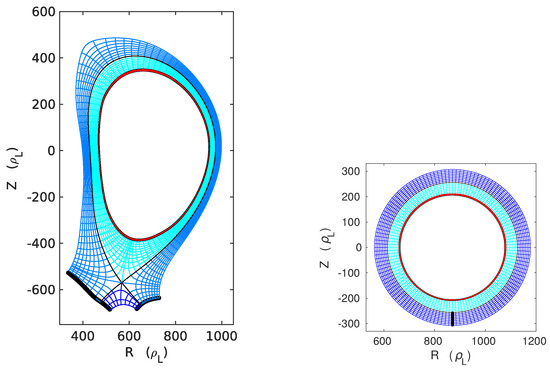
Figure 2.
(Left) COMPASS-like mesh grid used for TOKAM3X simulations. Displayed grid is coarser than the actual used by the code by a factor four, both in radial and poloidal direction. Toroidally, a quarter of the torus is simulated. Thick black line indicates divertor targets, where the Bohm’s boundary conditions are imposed. The region where the particle source is located, is highlighted in red. (Right) same plot for the limiter configuration.
TOKAM3X is based on a flux-surface aligned coordinate system, , where labels flux surfaces, is a curvilinear abscissa along the magnetic flux surface in the poloidal plane, and is the toroidal direction. The grid resolution in the space is in the divertor simulation (plus for the region below the X-point), and in the limiter one. The geometrical domain is subdivided in several subdomains, rectangular in the plane, connected to each other in the radial or in the poloidal direction. This division in subdomains allows the treatment of arbitrary axisymmetric magnetic topologies, including the single-null divertor configuration. In this case, by a proper choice of the domain subdivision [16], the X-point is a corner point, common to several subdomains communicating with each other. Since the magnetic field is calculated in the center of cells, the singularity in flux-aligned coordinates is by-passed.
TOKAM3X adopts a flux-driven approach: this means that no scale separation is assumed, and the background plasma is evolved together with the small-scale fluctuations. Initially, an artificial average profile is imposed (where all the normalized fields are set to 0, apart from T which is set to 1), then we let the system evolve freely. Gradients form thanks to the imposed particle source, and the plasma becomes turbulent when a critical value of the gradient is reached. Simulations are run for times longer than the characteristic confinement time (∼10) until the quantities N, and W, integrated over the whole domain, show small temporal variation () over a sufficiently long period of time.
3. Results
3.1. Deformation of Turbulent Structures Due to the X-Point
Interchange turbulence leads to turbulent structures which are quasi-field-aligned, because of the rapidity of parallel transport with respect to the cross-field one. More precisely, in our simulations . Assuming, at the first order, a structure perfectly aligned to a flux tube, one can study the spatial variation of the structure in the poloidal plane simply by knowing the magnetic field shape.
The divertor configuration introduces a saddle point for the poloidal flux, the X-point, leading to strong local deformations of the poloidal magnetic field, and ultimately on field-aligned structures. These effects have been quantified theoretically, assuming a certain magnetic field shape in the proximity of the X-point [23], and reproduced numerically in flux-tube simulations [24]. In TOKAM3X divertor simulations we observe turbulent structures whose shape in the poloidal plane varies strongly according to the position. In particular, in [25] we have verified that turbulent structures lying on the flux surface at the poloidal position are characterized by poloidal wavenumber
where the superscript indicates the outer midplane, and is the poloidal flux expansion. In (10), the dependence on the major radius comes from the inverse proportionality of the magnetic field with the major radius R. Equation (10) shows that structures become infinitely thin in the poloidal direction at the X-point. Since the total cross-section of the flux tube is conserved, filaments also become extremely stretched in the radial direction.
A second geometric effect is given by the magnetic shear. This geometric characteristic of the magnetic field deforms to a bigger extent the structures which are more extended radially. The typical shape of turbulent structures in the SOL, close to the X-point, of a COMPASS-like simulation, is visible in Figure 3.
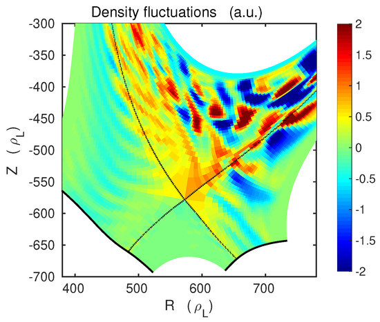
Figure 3.
Snapshot of density fluctuations in a COMPASS-like diverted simulation, with zoom on the divertor region.
One can notice from Figure 3 that in the vicinity of the outer target, structures get an elongated and sheared shape, so that they appear as finger structures pointing towards the outer target. This kind of shape was observed also by fast-imaging visible cameras in the MAST (Mega-Ampère Spherical Tokamak) divertor [26]. For the moment, this comparison can only be qualitative, since the light emission measured by fast-imaging cameras is actually a function of electrons density and temperature, and neutral density: these last two elements are not present in the simulation that we are analyzing. Therefore, in our isothermal simulations the emission would be only a function of electron density. Only a few attempts of comparison between fast cameras and numerical simulations have been carried out by other authors (e.g., [27]), relying on several assumptions. However, considering that temperature fluctuations have small phase shift with respect to density ones, the emissivity on lines is generally considered as a good indicator of electron density.
This qualitative comparison confirms that the nature of turbulence in the divertor is well described by TOKAM3X. We need however to inspect not only the shape of fluctuations in the divertor, but also their amplitude.
3.2. Fluctuations Amplitude in the Vicinity of the X-Point
In TOKAM3X simulations, and usually also in experiments, turbulent structures originate at locations close to the low-field side (LFS) midplane, as it can be expected from the ballooned nature of interchange turbulence. After propagating radially into the SOL, structures spread in the divertor region through parallel transport, as one can see from Figure 3. Filaments extend in the parallel direction up to the targets, progressively losing amplitude. On the LFS, the SOL region is in generally unstable towards interchange turbulence, since , even at locations lower than the X-point. Nevertheless, experiments have underlined the presence of a quiescent region in the divertor SOL, just outside the separatrix, where fluctuations amplitude is reduced. Several tokamaks, as the Mega Amp Spherical Tokamak (MAST) [28] and the Tokamak à Configuration Variable (TCV) [29], have shown the same feature. Thus, this phenomenon seems to be generalized, and common to all experiments with at least one X-point.
The cause of the quiescent region is clearly to be searched in the presence of the X-point. In the SOL region around the X-point, indeed, the connection length diverges, so that filaments get more easily decorrelated in the parallel direction. Moreover, for the deformation effect described previously, turbulent structures become extremely thin in the poloidal direction, so they tend to be damped more easily by diffusive mechanisms (density fluctuations damping ). Finally, the magnetic shear in this region is expected to decrease the linear growth rate of the interchange instability.
Magnetic shear is defined for limiter configurations as , where q is the safety factor of the flux surface, calculated as in [30]. The magnetic shear definition must be generalized when considering more complex geometries, as the divertor one: in regions as the divertor SOL and the Private Flux Region (PFR), in fact, r is ill-defined. Several generalized definitions can be found in literature (e.g., [31,32,33]), but there is no work, to our knowledge, that relates turbulence growth rates to one of these specific parameters. Therefore, we will use here a simpler and intuitive definition of the local magnetic shear. Using the expression for the safety factor in large aspect-ratio tokamaks, , we reformulate the definition of magnetic shear as:
We generalize then the definition of r by replacing it with the average curvature radius on the flux surface . We also replace the derivative in the radial direction with the derivative in the direction, finally obtaining:
This definition reduces to the simpler one in the limit of circular geometries. Figure 4 shows a map of the standard deviation of density fluctuations in the divertor region, along with the average density value, and the local shear calculated for the COMPASS-like geometry used in simulations. The ⟨⟩ operator stands for the average in toroidal direction and time, unless otherwise specified.
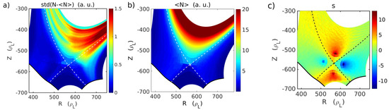
Figure 4.
(a) Standard deviation of density fluctuations sampled in time and toroidal direction, zoom on the divertor region. (b) Poloidal map of the average density. (c) 2D map of the local magnetic shear in the divertor region.
As visible in Figure 4a, within a radial distance of ∼15 from the separatrix, the standard deviation of density fluctuations drops suddenly by a factor at the poloidal location of the X-point. We are able thus, to recover the quiescent region feature observed in experiments. The quiescent region appears in all the TOKAM3X simulations with divertor configuration (see [34] for a TCV-like geometry), even if its extension can vary among different equilibria.
One can notice from Figure 4 that turbulence is strongly damped in regions where > ∼5. In the far SOL, where the shear is low, turbulent structures can connect again to the target. Turbulence damping seems, so, to correlate well with the presence of magnetic shear. This has been also noticed in TOKAM3X simulations where an artificial shear has been imposed in a limiter geometry [35]. We remark that the deformation experienced by the filament is an integrated effect, which depends on the position where the structure is generated, and on its propagation. In our simulations, most of the filaments are generated near the LFS midplane, so they are all subject, on average, to a similar shear effect.
We also notice from Figure 4a that density fluctuations are partially damped in the region of closed flux surfaces near the X-point, even if with a lower extent. As shown in Figure 4b, the average density decays radially, also at the X-point poloidal location. Nevertheless, one must notice that density is fairly constant poloidally, also near the last closed flux surface (LCFS): this means that poloidally, the ratio of the fluctuation amplitude with respect to the background value, is lowered close to the X-point. This is coherent with the fact that the turbulence damping mechanisms described above are also at play in this region. The low fluctuation level in the closed flux surface region around the X-point could be related to the formation of transport barriers, described in the next section.
3.3. Effects of a Transport Barrier on Edge Turbulence
TOKAM3X simulations in divertor configuration show the presence of spontaneous transport barriers (not forced by any physical parameter), which are absent in TOKAM3X limiter isothermal simulations run with the same set of physical parameters.
The macroscopic signature of a transport barrier is the local increase of radial gradients of plasma density: indeed, in absence of anomalous transport, less effective transport mechanism come into play, such as neoclassical transport. In Figure 5, we represent the radial profile of the density averaged over time and toroidal direction, for different poloidal locations.
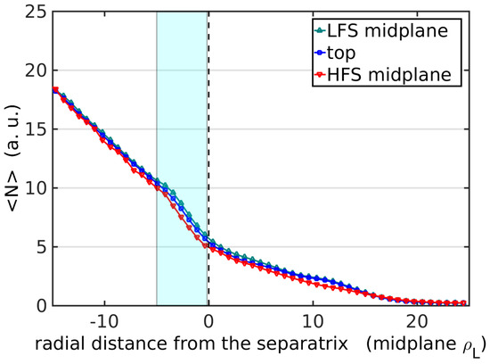
Figure 5.
Radial profiles of the density averaged over time and toroidal direction, for a COMPASS-like diverted geometry. The profiles are taken at the LFS midplane, at the top of the plasma (top), and at the High-Field Side (HFS) midplane. In evidence, the region affected by the barrier.
We notice from Figure 5 that there is a local increase in the density gradient in the closed flux surface region, near the LCFS. It is important to notice that the effect of the barrier on density profiles is extended on the whole flux surfaces which are affected. We observe this transport barrier in all the TOKAM3X divertor simulations, although its effect on average density profile can differ quantitatively. No sign of transport barrier has been detected in limiter simulations run with similar physical parameters, as it can be verified, for example, in [36].
We can quantify the efficiency of turbulent transport with the parameter , defined as in [37]:
where and are respectively the flux and the diffusive flux in the direction, averaged over the flux surface. Sometimes in literature the complementary parameter is used (e.g., in [38]). We consider the average fluxes on flux surfaces, since we are interested in the net particle transport across flux surfaces. Here the plays no role, because of its small divergence over a flux surface. In the closed flux surfaces region, we notice that
where ˜ indicates the fluctuating part of the field. The turbulent flux, so, approximates well the total flux. In a flux-driven system, the total cross-field flux averaged over a flux surface should be radially constant in the closed field lines, since there are no net parallel losses. Therefore, a decrease in the turbulent transport enhances the diffusive flux, leading to a lower index. Vice versa, in regions not affected by the barrier, . Figure 6a shows the coefficient, calculated for a given timespan.
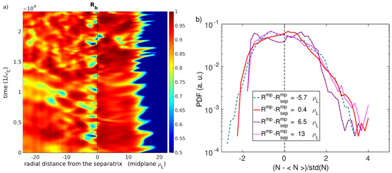
Figure 6.
(a) Turbulent transport efficiency coefficient , in function of the midplane radius and of time. The dashed line indicates the separatrix position. (b) Probability density fluctuations (PDFs) at four different radial positions, calculated at the LFS midplane. The corresponding values of the skewness, from radially inwards to radially outwards positions, are respectively , , and .
We can notice from Figure 6a that a mild transport barrier is active in the closed field lines, in the vicinity of the separatrix. The region affected by the transport barrier is thin, with a width of ∼5 . We remark that the drift-reduced model is at the limit of its applicability domain in this case, since this structure develops on few Larmor radii. From the numerical point of view, the barrier affects radially mainly five to eight points in our grid, highlighting the fact that a high resolution is necessary in this region to capture the phenomenon of the transport barrier. One can notice that the behavior of the barrier is intermittent in time: this reflects the fact that some structures manage to radially overcome the barrier, while others get damped while being in the barrier region.
In this simulation, turbulence carries on average around the of the flux in the barrier region. However, the standard deviation fluctuations of the turbulent transport efficiency value is around , and can decrease to up to the . In the innermost closed flux surfaces, instead, the turbulent flux carries more than the of the particles. Also, in the SOL, turbulent flux is dominant, but the total flux is decreasing because of the particles draining towards the divertor targets. After a characteristic decay length of around , comparable with the density decay length observed at the target, turbulent flux is almost completely decayed and becomes comparable, or even lower, than the diffusive flux. One can also notice from Figure 6a the propagation of turbulent events in the SOL, occurring with a frequency of around . The low efficiency of the transport barrier in reducing turbulent transport can be partially due to its small width, smaller than the average radial correlation length, which is around .
These characteristics of the transport barriers seem to have some similarities to the ones found in the 2D fluid turbulence code TOKAM2D in the work by Ph. Ghendrih et al. [39]. In that analysis, the curvature term, responsible for the interchange turbulence driving, was artificially suppressed in a localized radial region. The simulations revealed the presence of a transport barrier, whose coefficient had a bell-shape in the radial direction, given by the spreading of turbulence in the stable region (although in that case , much lower than the one found in divertor simulations). In divertor geometry, the transport barrier builds up in a zone where the driving terms are comparable with the rest of the domain. This suggests that a steady mechanism of turbulence damping is at play.
The transport barrier seems also to locally alter the statistical properties of turbulent fluctuations. Figure 6b represents the Probability Density Function (PDF) for different radial positions at the LFS midplane of the simulation. The probability density function of density fluctuations, which are usually generated at the innermost flux surfaces, have an almost Gaussian shape before encountering the barrier, and get increasingly positively skewed propagating radially outwards. However, the effects of the barrier are visible after the separatrix. As one can see from Figure 6b, the PDF calculated just outside the separatrix has a hollow profile: this suggests that while large-amplitude events can survive the barrier, small ones are more easily damped, and thus less probable in the near SOL. The usual, positively skewed shape of the PDF is re-established further in the SOL, as it was observed in former simulations in limiter configuration [36].
The factor is a global index of the efficiency of transport barrier over a flux surface. However, poloidally, turbulent structures do not behave homogeneously. Figure 7 shows the standard deviation of density and potential fluctuations at different poloidal locations.
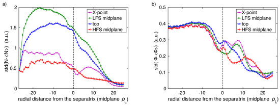
Figure 7.
(a) Radial profiles of the standard deviation of density fluctuations, plotted at different poloidal position. (b) Same plot for the electrostatic potential fluctuations.
As visible in Figure 7a, the density fluctuation level is lowered by roughly the in the closed flux surfaces, near the X-point. Moreover, at the same radial position, the level of fluctuation is lowered also at the LFS and at the HFS midplane, even though only by around the . This effect is even more visible on electrostatic potential fluctuations, whose amplitude is more homogeneous on the flux surface. We remark also that the relative decay of the amplitude of electrostatic fluctuations in the barrier region, around the , is stronger than the one observed on density fluctuations.
These elements suggest a non-local effect of the damping of turbulent structures around the X-point, which are connected to the LFS midplane by the parallel transport of particles and electric charge. Nevertheless, the magnetic shear is not the only element acting in the vicinity of the Last Closed Flux Surface, and the role of the other mechanisms, pointed out in Figure 1, must also be inspected.
3.4. The Role of Poloidal Shear in Suppressing Turbulence
One of the possible causes of turbulence suppression is the decorrelation of density and velocity fluctuations by means of the poloidal shear . This can happen only if the shear acts on time scales faster than the growth rate of the instability [3]:
Figure 8a shows the shear averaged over the flux surfaces in our divertor simulation. The same profile is traced for a simulation with limiter configuration for comparison.
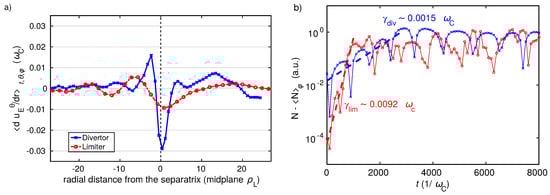
Figure 8.
(a) Radial shear of the poloidal velocity averaged in time and over the flux surface and remapped at LFS midplane in a COMPASS-like and in a limiter simulation. (b) Time trace of density fluctuations, calculated at the LFS midplane at , including the linear phase, in divertor and limiter configurations. Dashed lines indicate the exponential fit used to evaluate the linear growth rate.
The strongest shear is measured at the separatrix. This happens because the poloidal velocity suddenly changes direction between the closed field lines and the open field lines. In fact, in closed field lines the electric field is directed radially inwards, to balance the pressure gradient, while in the SOL the electric field is directed outwards because of the boundary conditions at the targets. We notice also that the shear can be 2–3 times stronger in divertor than in limiter configuration. This is due, at least partly, to the fact that in the divertor configuration the flux surfaces are more radially compressed at the LFS midplane, as visible in Figure 2.
Figure 8b shows the linear phase of turbulence, observed at the point in space where the growth rate was observed to be the largest in the divertor configuration. In particular, this point usually locates near the particle source, in the closed flux surfaces. In order to evaluate the linear growth rate independently from the evolution of the background density, we subtract the field averaged over the toroidal direction . As one can notice from Figure 8b, the maximum linear growth rate in divertor geometry is around . Positive and negative peaks are given by the fact that positive and negative fluctuations are advected through the fixed observation point by the drift. In limiter configuration, the linear growth rate for the interchange turbulence appears to be bigger by a factor ∼6 with respect to the divertor configuration: this difference is due to the different global curvature and magnetic shear, as pointed out in [40].
In divertor simulations, so, the shearing rate seems to be lower, or comparable with the growth rate of the instability at the point where turbulent structures form. Therefore, it may impact the amplitude of the fluctuations in steady state, but it does not prevent the formation of turbulent structures. However, turbulent structures propagate then radially, finally encountering the barrier region, where the condition (15) is clearly satisfied.
We notice from Figure 8a that the location where the shear peaks is slightly misaligned with respect to the actual location of the transport barrier. Nevertheless, the condition (15) is satisfied already at ∼5 inside the separatrix, where the barrier is located, so we cannot exclude, in these simulations, the importance of the shear. At the radial location where we observe the transport barrier, so, we have both the magnetic shear acting at the X-point, and possibly inducing non-local effects, and an shear spread around the flux surface. This situation is not comparable with limiter simulations, where the X-point shear is absent and the shear is generally lower than the linear growth rate, as visible in Figure 8a. The picture is complicated by the fact that the magnetic shear induced by the X-point, as explained in [8], can induce net poloidal flows (potentially sheared) by means of the Reynolds stress mechanism. In order to investigate more deeply the origin of the transport barriers, we evaluate in the next section the contribution of the Reynolds stress on the total fluxes in our simulations.
4. Discussion: The Role of Reynolds Stress in Generating Poloidal Fluxes
The radial profile of the poloidal velocity, and thus of the electrostatic potential, is determined by the vorticity balance (4). This balance equation contains the information about the conservation of the poloidal momentum. As described in [4], turbulence can drive ZF, by means of the Reynolds stress. This mechanism can be described, in the simplest way and in a simplified Cartesian geometry, by the equation:
where the coordinate x identifies the radial direction, y the poloidal one, and is the so-called Reynolds stress.
In TOKAM3X model, the radial derivative of the Reynolds stress is contained in the advection term in vorticity equation. The other terms, however, contribute as well to determine the equilibrium profile of the velocity. To investigate the impact of the Reynolds stress mechanism on the formation of the transport barrier, we run a divertor simulation with the same physical and geometrical parameters as the previously described one, and we artificially suppress the Reynolds stress term in the vorticity equation. The resulting profile of poloidal velocity is represented in Figure 9a.
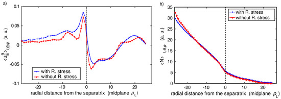
Figure 9.
(a) Radial profile of the poloidal velocity averaged on time ad over the flux surface in a COMPASS-like geometry, in the cases with and without Reynolds stress. (b) Comparison of the density averaged on the flux surface, in the two cases.
One can notice in Figure 9a that the poloidal velocity is slightly reduced in magnitude, in the case without Reynolds stress driving, and its radial derivative is weakly impacted. The amplitude of the transport barrier and the global equilibrium, are not affected, as shown in Figure 9b, by the absence of the advection term in the vorticity equation. This analysis suggests that the radial profile of the average poloidal velocity is mainly dominated by the linear terms in Equation (4): in particular, the average electric field tends to equilibrate the radial pressure gradient.
We have thus excluded the turbulence-driven ZF from the causes of the transport barrier build-up in our simulations. In order to identify, between the and the magnetic shear, the mechanism leading to the formation of the observed transport barrier, further simulations have been setup, in which an artificial magnetic shear is introduced in a simplified circular geometry: this is the subject of the work [35]. The results show, more clearly than in divertor simulations, that in isothermal cases, the shear plays a minor role in damping turbulent fluctuations, with respect to the magnetic shear, essentially confirming the central role of the magnetic shear in creating the transport barrier observed in this work.
5. Conclusions
TOKAM3X global simulations of electrostatic turbulence in tokamak edge plasma have been run in realistic divertor geometry. As previously found theoretically and experimentally, filaments get strongly elongated and poloidally thin in the X-point region, because of the large flux expansion.
A quiescent region, where the fluctuation level is drastically reduced, similar to the one observed in recent experiments, is found in the divertor SOL, close to the separatrix. The magnetic shear introduced by the X-point is pointed out as the possible cause for this damping. Indeed, the low poloidal field leads to large values around the X-point, so that dissipation processes tend to damp turbulent structures. More non-linear simulations, spanning different values of the magnetic shear, are needed to clarify this point. In the interpretation of the results here presented, one must consider the effects of the finite size of the grid cells. Near the X-point, in fact, turbulent structures can reach, in the poloidal direction, sizes comparable to the grid cell. This process is likely to introduce a cut-off in the possible range of scales describable by the code. Also, a strong numerical diffusion could intervene, smoothing the sharp gradients from one cell to the adjacent. The weight of the numerical diffusion in TOKAM3X simulations with divertor configuration, is currently being evaluated by means of the PoPe method [41], and the first results seem to show that numerical diffusion is of the same order of magnitude as the imposed physical one. Nevertheless, even if the nature of the dissipation of turbulent fluctuations around the X-point is still uncertain, this characteristic reproduces qualitatively well the experimental observations.
It is important to notice that in TOKAM3X divertor simulations, this local mechanism probably leads to a non-local effect, namely the reduction of the fluctuation amplitude over the last closed flux surfaces. Simulations have shown indeed the spontaneous formation of a transport barrier, namely not forced by any physical parameter, which increases the pressure gradient in the outermost zone of the confined plasma. This gradient steepening is associated with a reduction in fluctuation amplitude, which could be due to the magnetic shear at the X-point, or to the shear along the flux surface. The shear indeed appears to be strong near the separatrix, and comparable with the linear growth rate of the instability. The simulations carried out in absence of Reynolds stress seem to indicate that at least for the considered plasma parameters, the poloidal flows driven by turbulence have a little effect on the total poloidal velocity, and thus also on the formation of the transport barrier. Nevertheless, the fact that turbulence is mainly damped near the X-point region, and the slight misalignment of the location of the maximum shear with respect to the location of the transport barrier, seem to indicate the magnetic shear as the main cause of the transport barrier in the simulations. A further confirmation of this view has been recently given by the simulations carried out in [35], where an artificial magnetic shear is introduced in a simplified circular geometry.
Even if the observed transport barrier is mild, and does not lead to a bifurcation in the dynamical behavior of the system as in the L-H transition, it has characteristics in common with the experimentally observed edge transport barriers, as the localization near the separatrix and its narrow radial extension. The behavior of the dynamical system could potentially change significantly with the inclusion of the energy transport [17], and of self-consistent plasma-neutrals interactions [42]. Although the nature of the instability is not expected to change, in anisothermal simulations with divertor geometry we might observe higher potential background gradients in open and closed field lines, leading to higher shear values near the separatrix. This could potentially lead to stronger transport barriers, and consequently to steeper characteristics gradients, in a bifurcative dynamics. The capability of TOKAM3X, as well as of other codes of the same kind (e.g., [43,44]) to perform simulations with such complex models and realistic divertor geometries, will hopefully shed more light on the L-H transition dynamics. Nevertheless, the geometric effects of the X-point on turbulence here described might be an important element in the formation of the edge transport barriers, which seems to be linked both to plasma and magnetic field characteristics. The simulations here described will help, in the interpretation of more complete, and complex, simulations, and they are part of the necessary step-by-step process for the understanding of the edge transport barriers formation. Moreover, investigating the interaction between turbulent fluctuations and the magnetic X-point also contributes to the understanding of particles and heat flux deposition on targets. Indeed, the radial extent of the SOL region carrying most of the heat flux is comparable with the one of the observed quiescent regions. This aspect will be further studied in anisothermal simulations with divertor configuration.
Author Contributions
Conceptualization, D.G. and G.C.; methodology, P.T.; software, P.T., H.B., D.G. and E.S.; formal analysis, D.G., N.N., P.T. and P.G.; resources, E.S., G.C., P.T.; writing—original draft preparation, D.G.; writing—review and editing, G.C. and E.S.; supervision, G.C., E.S. and P.T.
Funding
This work has been carried out within the framework of the EUROfusion Consortium and has received funding from the Euratom research and training programme 2014–2018 and 2019–2020 under grant agreement No 633053 for projects WP15-ER/EPFL-05 and WP17-ER/CEA-08. The views and opinions expressed herein do not necessarily reflect those of the European Commission. The project leading to this publication has received funding from Excellence Initiative of Aix-Marseille University-AMIDEX, a French “Investissements d’Avenir” programme.
Acknowledgments
This work was granted access to the HPC resources of IDRIS, under the allocations i2015056912 and i20150242 made by GENCI, and of Aix-Marseille University, financed by the project Equip@Meso (ANR-10-EQPX-29-01) of the program “Investissements d’ Avenir”supervised by the Agence Nationale de la Recherche (National Research Agency).
Conflicts of Interest
The authors declare no conflict of interest.
References
- Martin, Y.R.; Takizuka, T.; The ITPA CDBM H-mode Threshold Database Working Group. Power requirement for accessing the H-mode in ITER. J. Phys. Conf. Ser. 2008, 123, 012033. [Google Scholar] [CrossRef]
- Hubbard, A.E. Physics and scaling of the H-mode pedestal. Plasma Phys. Control. Fusion 2000, 42, A15–A35. [Google Scholar] [CrossRef]
- Burrell, K.H. Effects of ExB velocity shear and magnetic shear on turbulence and transport in magnetic confinement devices. Phys. Plasmas 1997, 4, 1499–1518. [Google Scholar] [CrossRef]
- Diamond, P.H.; Kim, Y.B. Theory of mean poloidal flow generation by turbulence. Phys. Fluids B 1991, 3, 1626. [Google Scholar] [CrossRef]
- Ricci, P.; Rogers, B.N.; Brunner, S. High and Low-Confinement Modes in Simple Magnetized Toroidal Plasmas. Phys. Rev. Lett. 2008, 100, 225002. [Google Scholar] [CrossRef] [PubMed]
- Garbet, X. Instabilités, turbulence et transport dans un plasma magnetisé 2001. Ph.D. Thesis, University of Marseille, Marseille, France, 2001. [Google Scholar]
- Waltz, R.E.; Staebler, G.M.; Dorland, W.; Hammett, G.W.; Kotschenreuther, M.; Konings, J.A. A gyro-Landau-fluid transport model. Phys. Plasmas 1997, 4, 2482. [Google Scholar] [CrossRef]
- Fedorczak, N.; Diamond, P.; Tynan, G.; Manz, P. Shear-induced Reynolds stress at the edge of L-mode tokamak plasmas. Nucl. Fusion 2012, 52, 103013. [Google Scholar] [CrossRef]
- Ghendrih, P.; Ciraolo, G.; Larmande, Y.; Sarazin, Y.; Tamain, P.; Beyer, P.; Chiavassa, G.; Darmet, G.; Garbet, X.; Grandgirard, V. Shearing effects on density burst propagation in SOL plasmas. J. Nucl. Mater. 2009, 390, 425–427. [Google Scholar] [CrossRef]
- Ciraolo, G.; Ghendrih, P.; Sarazin, Y.; Chandre, C.; Lima, R.; Vittot, M.; Pettini, M. Control of test particle transport in a turbulent electrostatic model of the Scrape-Off-Layer. J. Nucl. Mater. 2007, 363, 550–554. [Google Scholar] [CrossRef]
- Rasmussen, J.J.; Nielsen, A.H.; Madsen, J.; Naulin, V.; Xu, G.S. Numerical modeling of the transition from low to high confinement in magnetically confined plasma. Plasma Phys. Control. Fusion 2016, 58, 014031. [Google Scholar] [CrossRef]
- Halpern, F.; Ricci, P. Velocity shear, turbulent saturation, and steep plasma gradients in the scrape-off layer of inner-wall limited tokamaks. Nucl. Fusion 2017, 57, 034001. [Google Scholar] [CrossRef]
- Chang, C.S.; Ku, S.; Tynan, G.R.; Hager, R.; Churchill, R.M.; Cziegler, I.; Greenwald, M.; Hubbard, A.E.; Hughes, J.W. Fast Low-to-High Confinement Mode Bifurcation Dynamics in a Tokamak Edge Plasma Gyrokinetic Simulation. Phys. Rev. Lett. 2017, 118, 175001. [Google Scholar] [CrossRef] [PubMed]
- Wagner, F.; Becker, G.; Behringer, K.; Campbell, D.; Eberhagen, A.; Engelhardt, W.; Fussmann, G.; Gehre, O.; Gernhardt, J.; Gierke, G.V.; et al. Regime of Improved Confinement and High Beta in Neutral-Beam-Heated Divertor Discharges of the ASDEX Tokamak. Phys. Rev. Lett. 1982, 49, 1408–1412. [Google Scholar] [CrossRef]
- Moret, J.M.; Anton, M.; Barry, S.; Behn, R.; Besson, G.; Buhlmann, F.; Burri, A.; Chavan, R.; Corboz, M.; Deschenaux, C.; et al. Ohmic H-mode and confinement in TCV. Plasma Phys. Control. Fusion 1995, 37, A215. [Google Scholar] [CrossRef]
- The TOKAM3X code for edge turbulence fluid simulations of tokamak plasmas in versatile magnetic geometries. J. Comput. Phys. 2016, 321, 606–623. [CrossRef]
- Baudoin, C.; Tamain, P.; Bufferand, H.; Ciraolo, G.; Fedorczak, N.; Galassi, D.; Ghendrih, P.; Nace, N. Turbulent heat transport in TOKAM3X edge plasma simulations. Contrib. Plasma Phys. 2018, 58, 484–489. [Google Scholar] [CrossRef]
- Galassi, D.; Tamain, P.; Bufferand, H.; Ciraolo, G.; Ghendrih, P.; Baudoin, C.; Colin, C.; Fedorczak, N.; Nace, N.; Serre, E. Drive of parallel flows by turbulence and large-scale E × B transverse transport in divertor geometry. Nucl. Fusion 2017, 57, 036029. [Google Scholar] [CrossRef]
- Braginskii, S.I. Transport Processes in a Plasma; Provided by the SAO/NASA Astrophysics Data System; Consultants Bureau: New York, NY, USA, 1965; Volume 1, p. 205. [Google Scholar]
- Hinton, F.L.; Horton, C.W. Amplitude Limitation of a Collisional Drift Wave Instability. Phys. Fluids 1971, 14, 116. [Google Scholar] [CrossRef]
- Dimitrova, M.; Dejarnac, R.; Popov, T.K.; Ivanova, P.; Vasileva, E.; Kovačič, J.; Stöckel, J.; Havlicek, J.; Janky, F.; Panek, R. Plasma Parameters in the COMPASS Divertor During Ohmic Plasmas. Contrib. Plasma Phys. 2014, 54, 255–260. [Google Scholar] [CrossRef]
- Stangeby, P.C. The Plasma Boundary of Magnetic Fusion Devices; Institute of Physics Publishing: Bristol, UK, 2000. [Google Scholar]
- Farina, D.; Pozzoli, R.; Ryutov, D. Effect of the magnetic field geometry on the flute-like perturbations near the divertor X point. Nucl. Fusion 1993, 33, 1315. [Google Scholar] [CrossRef]
- Walkden, N.R.; Dudson, B.D.; Fishpool, G. Characterization of 3D filament dynamics in a MAST SOL flux tube geometry. Plasma Phys. Control. Fusion 2013, 55, 105005. [Google Scholar] [CrossRef]
- Galassi, D.; Tamain, P.; Baudoin, C.; Bufferand, H.; Ciraolo, G.; Fedorczak, N.; Ghendrih, P.; Nace, N.; Serre, E. Characterization of tokamak edge plasma turbulence in 3D global simulations with divertor geometry. In Proceedings of the 44th EPS Conference, Belfast, UK, 26–30 June 2017. [Google Scholar]
- Walkden, N.; Harrison, J.; Silburn, S.; Farley, T.; Henderson, S.; Kirk, A.; Militello, F.; Thornton, A.; The MAST Team. Quiescence near the X-point of MAST measured by high speed visible imaging. Nucl. Fusion 2017, 57, 126028. [Google Scholar] [CrossRef]
- Wersal, C.; Ricci, P. Impact of neutral density fluctuations on gas puff imaging diagnostics. Nucl. Fusion 2017, 57, 116018. [Google Scholar] [CrossRef]
- Walkden, N.; Militello, F.; Harrison, J.; Farley, T.; Silburn, S.; Young, J. Identification of intermittent transport in the scrape-off layer of MAST through high speed imaging. Nucl. Mater. Energy 2017, 12, 175–180. [Google Scholar] [CrossRef]
- Walkden, N.R.; Labit, B.; Reimerdes, H.; Harrison, J.; Farley, T.; Innocente, P.; Militello, F.; The TCV Team; The MST1 Team. Fluctuation characteristics of the TCV snowflake divertor measured with high speed visible imaging. Plasma Phys. Control. Fusion 2018, 60, 115008. [Google Scholar] [CrossRef]
- Wesson, J. Tokamaks; Oxford University Press: Oxford, UK, 2004. [Google Scholar]
- Xanthopoulos, P.; Mikkelsen, D.; Jenko, F.; Dorland, W.; Kalentev, O. Verification and application of numerically generated magnetic coordinate systems in gyrokinetics. Phys. Plasmas 2008, 15, 122108. [Google Scholar] [CrossRef]
- Lewandowski, J.L.V.; Persson, M. Local magnetic shear in tokamak plasmas. Plasma Phys. Control. Fusion 1995, 37, 1199. [Google Scholar] [CrossRef]
- Nadeem, M.; Rafiq, T.; Persson, M. Local magnetic shear and drift waves in stellarators. Phys. Plasmas 2001, 8, 4375–4385. [Google Scholar] [CrossRef]
- Gallo, A.; Fedorczak, N.; Elmore, S.; Maurizio, R.; Reimerdes, H.; Theiler, C.; Tsui, C.K.; Boedo, J.A.; Faitsch, M.; Bufferand, H.; et al. Impact of the plasma geometry on divertor power exhaust: Experimental evidence from TCV and simulations with SolEdge2D and TOKAM3X. Plasma Phys. Control. Fusion 2018, 60, 014007. [Google Scholar] [CrossRef]
- Nace, N.; Tamain, P.; Baudoin, C.; Bufferand, H.; Ciraolo, G.; Fedorczak, N.; Galassi, D.; Ghendrih, P.; Serre, E. Impact of safety factor and magnetic shear profiles on edge turbulence in circular limited geometry. Contrib. Plasma Phys. 2018, 58, 497–504. [Google Scholar] [CrossRef]
- Tamain, P.; Bufferand, H.; Ciraolo, G.; Colin, C.; Serre, E.; Schwander, F. 3D Properties of Edge Turbulent Transport in Full-Torus Simulations and their Impact on Poloidal Asymmetries. Contrib. Plasma Phys. 2014, 559, 555–559. [Google Scholar] [CrossRef]
- Floriani, E.; Ciraolo, G.; Ghendrih, P.; Lima, R.; Sarazin, Y. Self-regulation of turbulence bursts and transport barriers. Plasma Phys. Control. Fusion 2013, 55, 095012. [Google Scholar] [CrossRef]
- Nace, N.; Perin, M.; Tamain, P.; Ciraolo, G.; Baudoin, C.; Futtersack, R.; Ghendrih, P.; Norscini, C. Turbulence Interaction with Driven Transport Barriers in the Scrape-Off Layer of Tokamaks. Contrib. Plasma Phys. 2016, 56, 581–586. [Google Scholar] [CrossRef]
- Ghendrih, P.; Sarazin, Y.; Ciraolo, G.; Darmet, G.; Garbet, X.; Grangirard, V.; Tamain, P.; Benkadda, S.; Beyer, P. Transport barrier fluctuations governed by SOL turbulence spreading. J. Nucl. Mater. 2007, 363, 581–585. [Google Scholar] [CrossRef]
- Galassi, D.; Tamain, P.; Baudoin, C.; Bufferand, H.; Ciraolo, G.; Fedorczak, N.; Ghendrih, P.; Nace, N.; Serre, E. Flux expansion effect on turbulent transport in 3D global simulations. Nucl. Mater. Energy 2017. [Google Scholar] [CrossRef]
- Cartier-Michaud, T.; Ghendrih, P.; Sarazin, Y.; Abiteboul, J.; Bufferand, H.; Dif-Pradalier, G.; Garbet, X.; Grandgirard, V.; Latu, G.; Norscini, C.; et al. Projection on Proper elements for code control: Verification, numerical convergence, and reduced models. Application to plasma turbulence simulations. Phys. Plasmas 2016, 23, 020702. [Google Scholar] [CrossRef]
- Tamaina, P.; Baudoinab, C.; Bufferanda, H.; Ciraoloa, G.; Fanc, D.-M.; Fedorczaka, N.; Galassib, D.; Ghendriha, P.; Luceab, B.; Marandetc, Y.; et al. Impact of self-consistent neutrals dynamics and particle sources on edge plasma transport and turbulence in 3D first principle simulations. In Proceedings of the 23rd International Conference on Plasma Surface Interactions in Controlled Fusion Devices, Princeton, NJ, USA, 18–22 June 2018. [Google Scholar]
- Paruta, P.; Ricci, P.; Riva, F.; Wersal, C.; Beadle, C.; Frei, B. Simulation of plasma turbulence in the periphery of diverted tokamak by using the GBS code. Phys. Plasmas 2018, 25, 112301. [Google Scholar] [CrossRef]
- Stegmeir, A.; Coster, D.; Ross, A.; Maj, O.; Lackner, K.; Poli, E. GRILLIX: A 3D turbulence code based on the flux-coordinate independent approach. Plasma Phys. Control. Fusion 2018, 60, 035005. [Google Scholar] [CrossRef]


© 2019 by the authors. Licensee MDPI, Basel, Switzerland. This article is an open access article distributed under the terms and conditions of the Creative Commons Attribution (CC BY) license (http://creativecommons.org/licenses/by/4.0/).