Abstract
Incompressible magnetohydrodynamic (MHD) turbulence under influences of the Hall and the gyro-viscous terms was studied by means of direct numerical simulations of freely decaying, homogeneous and approximately isotropic turbulence. Numerical results were compared among MHD, Hall MHD, and extended MHD models focusing on differences of Hall and extended MHD turbulence from MHD turbulence at a fully relaxed state. Magnetic and kinetic energies, energy spectra, energy transfer, vorticity and current structures were studied. The Hall and gyro-viscous terms change the energy transfer in the equations of motions to be forward-transfer-dominant while the magnetic energy transfer remains backward-transfer-dominant. The gyro-viscosity works as a kind of hyper-diffusivity, attenuating the kinetic energy spectrum sharply at a high wave-number region. However, this term also induces high-vorticity events more frequently than MHD turbulence, making the turbulent field more intermittent. Vortices and currents were found to be transformed from sheet to tubular structures under the influences of the Hall and/or the gyro-viscous terms. These observations highlight features of fluid-dynamic aspect of turbulence in sub-ion-scales where turbulence is governed by the ion skin depth and ion Larmor radius.
1. Introduction
Plasma turbulence is observed in various fields of science including fusion plasma, space plasma, liquid metals in some devices, and others, with considerable diversity in its nature. Magnetohydrodynamic (MHD) model is applicable to a wide range of these studies. The MHD model has been used for numerical studies of instability and transition to turbulence in fusion plasmas extensively, for example (see Ref. [1] and references therein). However, the MHD approximation breaks down for plasma motions with small collisionality, because this approximation is essentially based on the local equilibrium hypothesis. Additionally, some effects such as the two-fluid (Hall) effects and the finite Larmor radius (gyro-viscous) effects, which are retained in the original formulation for a collisional plasma by Braginskii [2], are neglected in the MHD model.
For some numerical studies of instability and turbulence simulations where these neglected effects are important, an extended MHD model is adopted instead of the traditional MHD model [3,4,5]. However, nonlinear simulations of the extended MHD model with the Hall and gyro-viscous terms often require a large number of grid points and an extremely small time step width. This is closely related with the dispersive natures of the extended MHD model. The presence of the Hall term leads to propagation of whistler waves along the magnetic field, and restricts time steps very severely. The gyro-viscosity is closely related with drift wave instability, and has been validated for the Q-machine [6]. In addition, this effect is sometimes expected to stabilize a Rayleigh–Taylor (RT) type instability (including interchange and ballooning instability) [7,8,9]. However, fully nonlinear simulations of the RT instability show that the gyro-viscosity can enhance velocity shear and bring about broad-band excitation of Fourier components both in space and in time through secondary Kelvin–Helmholtz-like instability, making simulations much more unstable [10]. Nevertheless, instability and turbulence simulations by the use of the extended MHD model are meaningful both for studying physics of turbulence and for development research of a plasma facility because they can clarify some physics of instability and turbulence associated with the ion-skin-depth and ion Larmor radius, and provide more precise information than MHD simulations. Despite the incompleteness of the extended MHD model for plasma with small collisionality and the broad-band nature, extended MHD simulations are less expensive and affordable in a smaller HPC machine in comparison to kinetic (five- or six-dimensional) simulations. Thus, extended MHD simulations can contribute to understanding the physics of plasmas through less expensive computations over a wide range of parameters. In other words, an extended MHD simulation can be a good compromise between accuracy of physics and computational cost in many studies.
There are two approaches for overcoming the stiff and broad-band natures of the extended MHD simulations. The first approach is discarding the Hall and gyro-viscosity through the drift-ordering. Drift-ordered extended MHD equations such as the Heizeltine–Meiss model [3] are often used in nonlinear instability simulations in fusion plasmas. Since the ordering is made based on an assumption of some characteristic quantities, nonlinear simulations that violate the assumption are not validated. The second approach is adopting a semi- or fully implicit scheme in time-marching to overcome the restriction on very small time-step-width in a simulation [4,5]. However, this approach does not improve the demand for a high spatial resolution in an extended MHD simulation. On the contrary, the demand of a spatial resolution can even restrict applicability of the (semi-)implicit numerical approach through a large cost or a slow convergence of matrix solver, for example.
Although both approaches have artificial natures and difficulties in treatment of a small-spatial and short-time scale, this does not matter when relatively large-scale and long-time-scale motions are our interest. However, this can have significant influences on physics when we study turbulence and/or nonlinear evolution of short-wave instabilities such as interchange or ballooning modes. Recently, we proposed a third approach that mitigates the demand for the high resolutions and enables quicker computations: large eddy simulation (LES) approach for a simulation of plasma with a very small collisionality [11,12]. In an LES of fluid simulation, the artificial natures in the small and/or short scales appear as a phenomenological model, or sub-grid-scale (SGS) model, which represent roles of the scales smaller than the grid width to the scales larger than the grid width [13]. Virtues of the LES approach are that the SGS term can influence simulations only in a fully nonlinear or turbulent stage without contaminating the preceding linear instability stage and that we can make the time step width larger than full simulations by enabling a high-Reynolds-number turbulence simulation by a relatively small number of grid points.
The purpose of this paper is to present direct numerical simulations (DNS) of homogeneous and isotropic turbulence with and without the Hall and gyro-viscous terms, and deepen our understanding of basic natures of turbulence, specifically of small scales, under influences of these terms so that the understanding of small scales helps the three numerical approaches discussed above, ordering, a semi/full implicit method, and LES approach, with appropriate physical insights. Homogeneous and isotropic turbulence maintains some distance from application targets such as magnetically confined fusion problems. However, studying isotropic turbulence is one of the best approaches to deepen the understanding of the terms added to the MHD equations since this allows us to make use of various knowledge and analysis methods in turbulence of fluid mechanics (see, e.g., Refs. [14,15,16,17]). We concentrate on incompressible fluid in this article, although the extended MHD model is usually accompanied by fluid compressibility as well as finite variation of the mass density and the pressure. Even though some important aspects of plasma dynamics such as compressible modes (this is closely related with the stiffness of the equations) and dia-magnetic drift as well as gyro-viscous cancellations are lost by the incompressible assumptions, this assumption allows us to concentrate on acquiring basic insights into turbulent motions under influences of the velocity-gradient part of the gyro-viscosity.
2. Equations, Numerical Models, and Parameters
The incompressible extended MHD equations can be described as
The four symbols, , , , and are for the ith components of the magnetic field, the electric field, the current density, and velocity field vectors, respectively. The scalar variable p is the pressure which is determined by the incompressible condition in Equation (2). For a later use, the three components of the vorticity field are defined here as . The symbols and denote the Kronecker’s delta and the Levi–Civita’s anti-symmetric tensor, respectively. The symbol is the rate-of-strain tensor. The sum of 1, 2, and 3 is taken for repeated suffixes of the vector and tensor variables. The symbol is the Hall parameter, which indicates the ratio of the ion skin depth to the system size. The symbol represents the non-dissipative part of the Braginskii’s stress tensor (gyro-viscous tensor) [2],
The symbol is the ratio of the ion Larmor radius to the system size. See Table 1 for nomenclature. Obviously, the presence of the mean magnetic field is assumed in the derivation of the gyro-viscous tensor, and the formulation for the mean magnetic field introduces the anisotropy to the equations of motions in Equation (1). However, it turns out later that this term does not provide a strong anisotropy. We also note here that the thermodynamic pressure (or the mass density and temperature) is multiplied by Equations (7)–(12) in the original definition of the gyro-viscosity. Because of the incompressibility assumption, however, we have replaced the thermodynamic pressure by a constant value and have included the constant pressure in . In exchange for the linearization of the gyro-viscosity, we can focus on the effects of the velocity gradient in the gyro-viscous tensor on turbulence.

Table 1.
Nomenclature.
Equations (1)–(6) were normalized by a reference length scale , magnetic field strength , mass density ( and are the ion mass and the number density, respectively), and Alfvén velocity where is the vacuum permeability. The symbols and are magnetic diffusivity, and shear viscosity, respectively. We can understand and as the reference Reynolds number and the Lundquist number, respectively. Physical parameters in DNS are shown in Table 2.
Table 2.
Parameters in direct numerical simulations (DNS).
In these simulations, the dissipation scale was smaller than the ion skin depth and the ion Larmor radius. The Hall and gyro-viscous parameters were chosen so that they represent the ratios of the ion skin depth and the ion Larmor radius to the system length typically seen in the Large Helical Device fusion experiments [18,19], expecting application of the knowledge in this paper to numerical simulations of magnetically confined fusion plasma. The other two parameters, viscosity and the resistivity, were determined so that the DNS can achieve numerical convergence. Although these two parameters should be much smaller for fusion experiments or other applications such as space plasmas, this simulation study can provide some basic information on plasma turbulence. We come to the ratio of the viscosity and the resistivity at the end of this paper.
Equations (1)–(6) were solved numerically by means of the pseudo-spectral technique and the fourth-order Runge–Kutta–Gill technique under the periodic boundary condition.
The aliasing errors were removed by the -truncation method spherically in the Fourier space. See Appendix A for the validation of the simulation code. Initial velocity and magnetic fields were given by the energy spectrum proportional to ( in this paper) and random phases.
3. Numerical Result
3.1. Time Evolution of Energies
Firstly, we compared the time evolution of the kinetic and magnetic energies among the MHD, Hall MHD, and extended MHD models. Figure 1 presents the mean values of: (a) the kinetic energy ; and (b) magnetic energy , in the six runs except iHMHD-3. In the time evolution of the energies, we did not observe a clear difference among the models. The kinetic energy keeps decaying monotonically. The monotonic decay is caused not only by the viscous dissipation but also by the energy transfer from to associated with the dynamo process. On the other hand, the magnetic energy grows at first by receiving the energy from through the dynamo action, and then decays. Although we omit the plots of , the total energy decays slowly and monotonically thoroughly by the by the energy dissipation. These processes appear almost the same among the three models.
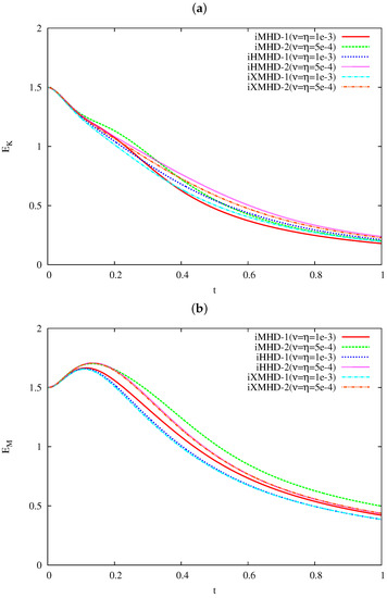
Figure 1.
Time evolution of: (a) the kinetic energy ; and (b) the magnetic energy .
The Taylor’s micro-scale Reynolds numbers of the velocity and magnetic fields are shown in Figure 2a,b, respectively. The velocity Reynolds number decays slowly. With respect to the three runs with small dissipative coefficients (runs iMHD-2, iHMHD-2, and iXMHD-2), at the final state. (Strictly speaking, still continues to decay but the decay is very slow at .) In contrast to the slow decay of , the magnetic Reynolds number reaches a statistically steady state for the three runs as soon as . The difference between the decays of the two Reynolds numbers can be understood as the consequence of the energy transfer from to . Since the dynamo effect keeps the energy transferring from to , both and keep decreasing. In the magnetic field, the energy transfer from and the energy dissipation by the resistivity can balance at a range of scales including the Taylor’s micro-scale despite the magnetic energy due to the dissipation, for . Consequently, stays almost constant while decays. Hereafter, we focus on the time as a fully relaxed state in the decaying simulations.
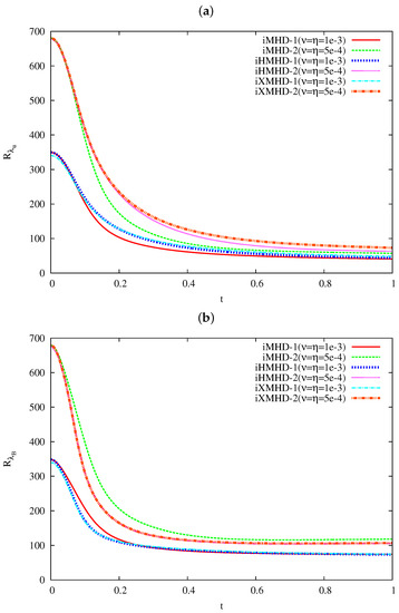
Figure 2.
Time evolution of the Taylor’s micro-scale Reynolds number on (a) the velocity and (b) magnetic fields.
3.2. Hall and Gyro-Viscous Effects in the Fourier Space
Energy spectra of MHD, Hall MHD, and extended MHD simulations are compared at in Figure 3. In Figure 3a, the kinetic energy spectrum of runs iMHD-1, iMHD-2, iHMHD-2, and iXMHD-2 are presented where and denotes the shell average in the Fourier space and a Fourier coefficient, respectively. Since the energy has been transferred from the kinetic energy to the magnetic energy, has been attenuated sufficiently until over a wide range of the wave-numbers, and the energy spectrum does not have a clear inertial sub-range.
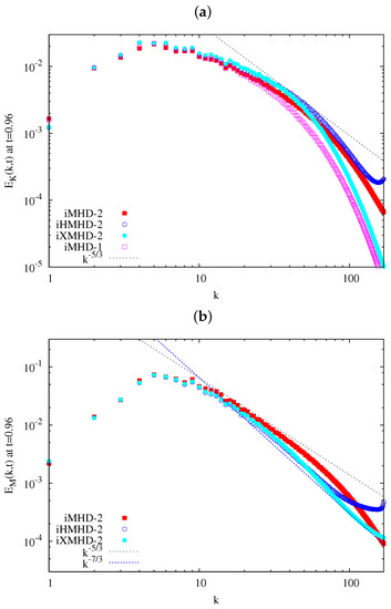
Figure 3.
Energy spectrum: (a) ; and (b) at .
We found that in iXMHD-2 is attenuated more sharply at than that in iMHD-2 (the same viscosity and resistivity as iXMHD-2), and even more sharply than iMHD-1 (the viscosity and resistivity are larger than those of iXMHD-2). In other words, the attenuation of of iXMHD-2 is much sharper than that of the other runs, indicating that the gyro-viscosity attenuates at a narrower range than a normal viscosity, working like a hyper-diffusivity. We must note again that the gyro-viscosity is non-dissipative part of the stress tensor in Braginskii’s formulation [2]. However, the linearization of the gyro-viscosity due to the incompressible assumption changes this term from non-dissipative to dissipative.
In Figure 3b, the magnetic energy spectrum of runs iMHD-2, iHMHD-2, and iXMHD-2 at is shown. Being sustained by the energy input by the dynamo action, the energy level of is higher than that of almost at all k. It has been reported earlier that the Hall term brings about a new scaling law (sub-inertial scaling region) in the sub-ion scale , in addition to the primary scaling region of Kolmogorov’s (or can be the Iroshnikov–Kraichnan )-law [20,21,22].
We found that the tail of of run iHMHD-2 is raised at . This is due to the Hall term enhancing the forward-energy-transfer through its quadratic nature to the magnetic field, as has been discussed in earlier works [20,23]. (A small raise in of run iHMHD-2 in the same wave-number region is considered as the consequence of the raise of .) Consequently, the resolution of the run iHMHD-2 is insufficient. Thus, we omit the wave-number region hereafter from our discussion. However, the raise of the tail in does not affect the qualitative discussion in this paper crucially, and thus we analyze run iHMHD-2 instead of iHMHD-3, for ease of comparison with the runs iMHD-2 and iXMHD-2. See Appendix A for a comparison of the spectra and the energy transfer functions of the runs iHMHD-2 and iHMHD-3.
Although the scaling region is not very clear in Figure 3b, we consider that the wave-number region can be the sub-inertial scaling region. While the scaling region of in iHMHD-2 and iXMHD-2 are occupied only by -law, the spectrum consists of both and regions in our earlier work [20]. We consider that the difference between this work and the earlier work comes from the change of the initial spectrum profile.
In this paper, we give the initial velocity and magnetic fields by the energy spectrum proportional to for . On the other hand, the initial fields in the earlier works have been given by the energy spectrum proportional to for . The change of the initial spectrum shape causes the proximity of the energy peak at and the sub-ion-scale (), and leads to the disappearance of -like region in runs iHMHD-2 and iXMHD-2. On the contrary, in run iMHD-2 shows a -like region of the absence of the Hall term. Consequently, the magnetic spectrum is more energetic in iMHD-2 than in iHMHD-2 (and iHMHD-3, equivalently). Although pursuing the reason for the disappearance of the -like primary sub-range may be interesting, this does not necessarily disturb our purpose in this paper, deepening an understanding of roles of the gyro-viscosity to turbulence. Note that the tail of is not raised very much in the run iXMHD-2 while it is raised in the run iHMHD-2. Although the Hall term excites the high-wave-number components in the magnetic field as in iHMHD-2, the gyro-viscosity in the equations of motions suppresses not only the high-wave-number components of the velocity field but also those of the magnetic field, indicating that the suppression of the high-wave-number components in the velocity field can lead to suppression of the high-wave-number components of the magnetic field.
In Figure 4, the energy transfer functions in the right-hand-side (rhs) of the equations of motions (Equation (1)) are compared among the runs: (a) iMHD-2; (b) iHMHD-2; and (c) iXMHD-2 at . The rhs terms in the equations of motions are grouped into the three parts, the advection term , the Lorentz force , and the gyro-viscous part which appears only in the extended MHD simulations. The transfer functions corresponding to these terms are defined according to a standard manner in fluid mechanics [15,16]. (See also Ref. [20] for the transfer functions of the Hall MHD equations.) The functions associated with the pressure gradient (which is always zero in the incompressible fluid) and the normal viscosity are omitted from the figure. We do not normalize the transfer functions by the Kolmogorov length scale and energy dissipation rate because the definition of the dissipation scale is ambiguous in the extended MHD equations because of the presence of the gyro-viscosity.
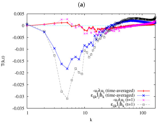
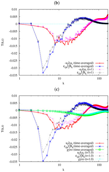
Figure 4.
Kinetic energy transfer functions at in the runs: (a) iMHD-2; (b) iHMHD-2; and (c) iXMHD-2, for the time-average over and for the time snap-shot .
In the figures, the transfer functions averaged over the period as well as the time snapshot of the functions at are presented so that the time-variation of the functions can be seen easily. The comparison between the time-averaged transfer function and the snap-shot shows that the snap-shot can give qualitative natures of the three kinds of turbulence, because plasma is in a statistically steady and fully relaxed state.
The magnitude of the transfer functions in Figure 4a are larger than those in Figure 4b,c. We also found that the sign of the transfer function associated with the advection is different between Figure 4a and Figure 4b,c. This term is positive at two regions, and , and negative at of the run iMHD-2 in Figure 4a. (As has been stated already, we exclude the region from the discussions because of the insufficiency of the run iHMHD-2, while the runs iMHD-2 and iXMHD-2 are considered converging numerically since the energy spectra and are attenuated rapidly toward large k, as shown in Figure 3. See Appendix A for the transfer function of iHMHD-3, a simulation with the same computation with iHMHD-2 but with a larger number of grid points, .) The existence of the positive region indicates that there is a backward-transfer of the energy toward this region. In contrast to Figure 4a, the transfer functions in Figure 4b,c show a typical forward-transfer-dominant profile similar to the transfer function observed in Navier–Stokes turbulence: negative in low-wave-number side and positive in high-wave-number side. Relative importance of the advection term and the Lorentz force in the energy transfer are also different among Figure 4a–c. The absolute value of the transfer function on the advection term is about of the transfer function on the Lorentz force in Figure 4a, while the ratio is about in Figure 4b,c.
Here, we pay attention to a difference of the energy transfer functions between Figure 4a and Figure 4b,c at moderate or high wave-number regions. The energy transfer by the advection term increases monotonically at the wave-number region in Figure 4a while the function does not necessarily increase monotonically in Figure 4b,c. The energy transfer by the Lorentz force also increase at the wave-number region in Figure 4a, while the transfer function increases at and decreases at , becoming almost zero at the highest wave-number in Figure 4b,c.
The transfer function associated with the gyro-viscosity is shown only in Figure 4c. The plot of the gyro-viscosity shows that the gyro-viscosity works as a sink of the kinetic energy at every scale. The wave-number , where the transfer function for the gyro-viscosity is minimum, gives a typical characteristic length scale of the velocity gradient.
In Figure 5, the transfer functions in the rhs of the magnetic field Equations (4) and (6) are compared among the runs: (a) iMHD-2; (b) iHMHD-2; and (c) iXMHD-2 at . The rhs terms in Equations (4) and (6) are re-arranged into the advection term and the magnetic-field-stretching term by the (electron) velocity , where is the electron velocity. Since in the MHD model, is equivalent to the velocity in iMHD-2. The two transfer functions on the advection and the stretching terms are defined in the same manner as in the above. Basically, the profiles of both the advection and stretching transfer functions look similar among the three panels, although the absolute values of the transfer functions of Figure 5a are about three times larger than those in Figure 5b,c. All of the three panels show that the two energy transfer functions are positive at and/or in the three runs, although the values are very small in iMHD-2. The two transfer functions are negative from to or higher, and become positive finally in the high wave-number region in the three panels. However, the energy transfer associated with the looks somewhat different qualitatively between Figure 5a and Figure 5b,c at .The energy transfer by this term is nearly zero at in Figure 5b,c, changing its sign at some k, while this term is almost constant and positive in Figure 5a. Thus, the magnetic field stretching by the electron velocity is not very active in this region in Figure 5b,c, and can contribute to either forward- or backward-energy transfer depending on some conditions. Clarifying this condition is left for future studies.
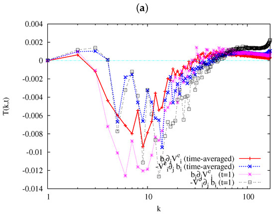
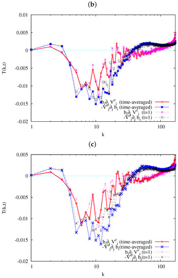
Figure 5.
Magnetic energy transfer functions at in the runs: (a) iMHD-2; (b) iHMHD-2; and (c) iXMHD-2, for the time-average over and for the time snap-shot .
3.3. Vorticity and Current Structures
Now, we examine vorticity and current density fields as the representatives of turbulent field.
In Figure 6, probability density functions (PDFs) of the three vector components: (a) ; (b) ; and (c) in the runs iMHD-2, iHMHD-2, and iXMHD-2 are shown at . Although a PDF is usually normalized by the deviation of a quantity in studies of turbulence, we do not normalize the PDFs in this figure because we aim at comparing the PDFs among different models.
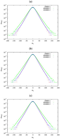
Figure 6.
The PDFs of the three vector components: (a) ; (b) ; and (c) in the runs iMHD-2, iHMHD-2, and iXMHD-2 at .
See Table 3 for the skewness , the kurtosis , and the standard deviation (, , or ) of the three vorticity vector components to compare how sharp the plots are.
Table 3.
Quantities for the sharpness of the three vorticity vector components.
All the plots in Figure 6 are non-Gaussian, showing a sharp triangular peak (except a very narrow region of zero-vorticity) and long tails at the high-vorticity regions. Obviously, the PDFs in Figure 6a–c show that the vorticity field of the run iHMHD-2 is much more intermittent than the other two runs. Although the Hall term influences only the magnetic field directly, the Hall term is considered to have excited the high-vorticity events through the Lorentz force. From the point of views on the small-scale excitation, the generation of high-vorticity events in iHMHD-2 can be related with a large forward energy transfer at observed in Figure 4b. The iXMHD-2 run also has the Hall term. However, it is considered that the hyper-diffusivity nature of the gyro-viscosity suppressed the high-vorticity events.
We found that outline of the PDFs of the runs iMHD-2 and iXMHD-2 are not necessarily the same as each other completely, although the difference is small. A difference between the MHD and extended MHD model can be seen at ( about ; see Table 3 for the values of ). The profile of the PDF of iMHD-2 at is convex and more parabolic than that of the iXMHD-2, which is concave there. The PDF of the run iXMHD-2 is lower than that of run iMHD-2 at and larger at . Thus, the probability density with moderate (large) of iXMHD-2 is smaller (larger) than that of iMHD2. In this sense, the turbulent vorticity field in the run iXMHD-2 is more intermittent than that in the run iMHD-2. Although the difference of the PDFs is small between the PDFs of iMHD-2 and iXMHD-2, the difference can become larger once the Reynolds numbers become larger, because the maximum vorticity in a simulation becomes larger for a higher Reynolds number. Since the probability density of large- events in iXMHD-2 are larger than that of iMHD-2, the extended MHD simulation requires finer spatial and temporal resolutions than the MHD simulation to resolve these high-vorticity events even though the energy spectrum is attenuated sharply as in Figure 3. The small differences between PDFs of runs iMHD-2 and iXMHD-2 may come from the nature of the gyro-viscosity to make a shear layer thinner, and be one of the reasons the extended MHD model is sometimes stiffer than the MHD model. We come to this point, with the reason we pay attention to the small differences, in the last section.
In Figure 7, PDFs of the three vector components: (a) ; (b) ; and (c) in the runs iMHD-2, iHMHD-2, and iXMHD-2 at are shown. See Table 4 for S, K, and the standard deviation of the three current-density components. While the tails of the PDFs are stretched, peaks of the PDFs are more Gaussian-like than those of the vorticity in Figure 6. Note that the tails of the high-current regions are more populated in the PDF of iMHD-2 than that in iHMHD-2. This is exactly opposite to our previous computations in Ref. [20]. We consider that this should be related with the change of the magnetic energy spectrum in Figure 3b, as mentioned above. The magnetic energy spectrum of iMHD-2 is larger than that of iHMHD-2 and iXMHD-2, while the slope of the spectrum of iMHD-2 is less steep than that of iHMHD-2 and iXMHD-2. Thus, the gradient of the magnetic field of iMHD-2 should be larger than that of the other runs, and can generate higher current density event.
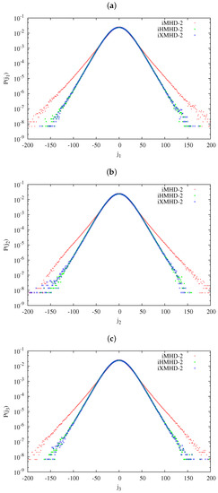
Figure 7.
The PDFs of the three vector components: (a) ; (b) ; and (c) in the runs iMHD-2, iHMHD-2, and iXMHD-2 at .
Table 4.
Quantities for the sharpness of the three current density vector components.
We found here that neither PDFs of the three vorticity components in Figure 6 nor those of the three current vector components in Figure 7 in run iXMHD-2 show a clear anisotropy. To clarify this point, the PDFs of the three components of the vorticity and the current in run iXMHD-2 are shown in Figure 8a,b, respectively. In this figure, the PDFs are normalized by the deviation ( for Figure 8a and for Figure 8b; ). Because of the anisotropy in the gyro-viscosity in Equations (7)–(12), the PDF of could be different from and . The current vector component () could also posses an anisotropy as well. However, the plots for all the three vector components in Figure 8a,b collapse almost completely to each other. Since the difference appears at a high-current region, it can be considered as one of the origins of the demand for a high numerical resolution in an extended MHD simulation. Since our turbulence simulations are carried out without the mean magnetic field, the formal anisotropy in Equations (7)–(12) does not work effectively. In this sense, we describe this turbulent field as approximately isotropic.
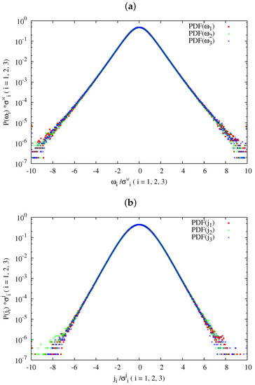
Figure 8.
The PDFs of the three components of: (a) the vorticity and (b) the current in run iXMHD-2 at , normalized by the deviation for (a) and for (b).
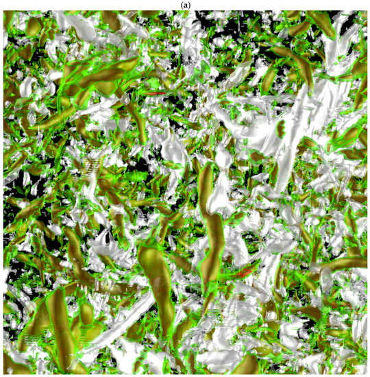
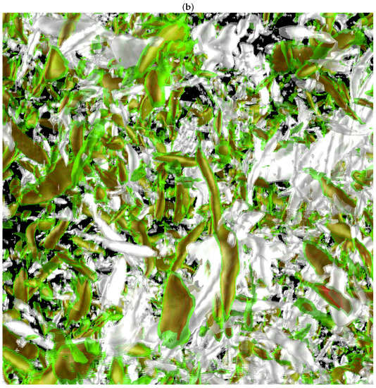
Changes of the vorticity and the current density fields in turbulence due to the Hall and gyro-viscous terms can be seen more directly by visualizing the entrophy density and the squared current density . In Figure 9, isosurfaces of these quantities in the runs: (a) iMHD-2; (b) iHMHD-2; and (c) iXMHD-2 are presented. The thresholds of the isosurfaces are given by the three times of the deviation above the average value of each quantity. As is well known, the isosurfaces of the two quantities in MHD turbulence often take thin sheet-shapes, vortex and current sheets, as shown in Figure 8a (see also the textbook by Biskamp [24] and references therein.) However, these structures are changed in Figure 9b,c. There are many vortex tubes and very small pieces of the current sheets in Figure 9b,c.
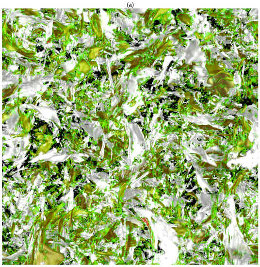
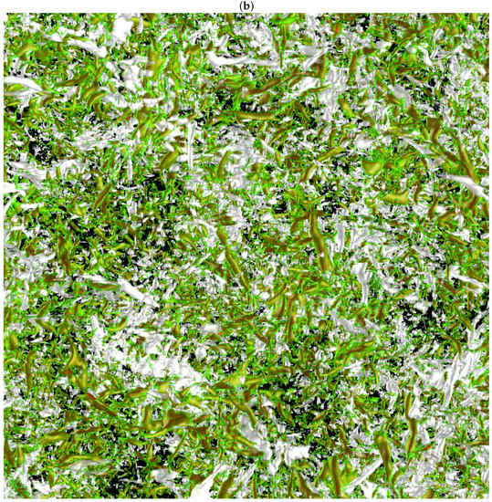
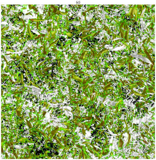
Figure 9.
Isosurfaces of the enstrophy density (green) and the current density (grey) in the runs: (a) iMHD-2; (b) iHMHD-2; and (c) iXMHD-2. The thresholds of the isosurfaces are given by three times the deviation above the average value of these quantities. The isosurfaces were drawn using the VISMO in-situ visualization library [27].
The difference of Figure 9a from Figure 9b,c can be partially understood as the Hall effects. We reported a transition of the spatial structures induced by the Hall term in homogeneous and isotropic turbulence [20]. The introduction of the Hall term changes the frozen-in condition of the magnetic field to velocity field in the limit of ideal (zero-dissipation) MHD equations. The magnetic field in the Hall MHD equations is frozen to the electron velocity field in the limit of zero-dissipation, so that the current field can be separated from the (ion) velocity field. Furthermore, the Hall term excites high wave-number Fourier components of the magnetic field and enhances the dissipation there in the case of turbulence in [20]. Since the velocity (vorticity) field is free from the restriction by the magnetic (current density) field through these processes, the vorticity field is enabled to roll up from sheets to tubes, as shown in Figure 9b,c.
A new finding in this visualization is in the current structures. Isosurfaces of I appear as many small pieces of sheets, as shown in Figure 9b,c. However, we find that some of the isosurfaces of I are tubular, not sheets, being separated from tubular vortices. (A part of Figure 9b,c is magnified in Figure 10a,b, respectively, to observe current tubes more closely.) A current sheet is closely related with some important physics such as magnetic reconnection, and has been a major and important structure in plasma physics [24]. On the other hand, there have not been many reports on tubular currents.
One possible understanding regarding the appearance of the current tubes is that current sheets are entrained into roll-up of strong vortices from sheets to tubes before the current density form current sheets. Since a current structure can travel much faster than a vortex structure when the Hall term is finite (consider whistler waves, for example), a current structure can be separated from a vortex tube either in the course of vortex-roll-up or after the roll-up process. The former process can result in formation of a current sheet independently from a vortex tube. On the other hand, the latter process can result in formation of a current tube, which travels along the magnetic field line away from the vortex tube, which has given the tubular shape to the current field.
Another possible understanding is the formation of current tubes associated with some specific types of magnetic reconnection [25,26]. While the current tubes can be originated by these magnetic reconnection, we need careful studies on the possibility. We must clarify whether these types of magnetic reconnection can occur frequently in the course of time evolution of turbulence, and whether these types of magnetic reconnection result in formation of the turbulent current tubes we have presented above. Furthermore, if these types of magnetic reconnection can happen frequently, we should study why they do not happen in simulations starting from another type of initial spectrum [20] or other forced turbulence studies. Since the study of the origin of the current tubes exceeds the scope of this article, we leave this as a future subject.
4. Concluding Remarks
Incompressible magnetohydrodynamic (MHD) turbulence under influences of the Hall and the gyro-viscous terms was studied numerically. Direct numerical simulations of freely decaying, homogeneous and approximately isotropic turbulence governed by incompressible MHD, Hall MHD, and extended MHD models were carried out for parameter sets such that the dissipation scale is smaller than the ion skin depth and the ion Larmor radius. The comparisons among the three models revealed some basic roles of the Hall term and the gyro-viscosity under the incompressible assumption. The gyro-viscosity can work as a kind of hyper-diffusivity in incompressible turbulence simulations. While the Hall term excites the high-wave-number components of the magnetic field, the gyro-viscosity can suppress the high-wave-number components. Backward energy transfer in the equations of motions can be suppressed both in the Hall and in the extended MHD models.
We have found in the analysis of the PDFs of the vorticity that the extended MHD turbulence can be more intermittent than that in MHD turbulence, even though the gyro-viscosity suppresses turbulent actions at high wave-numbers. These observations in the PDF can be closely related with other theoretical aspects of turbulence intermittency such as the anomalous scaling. With respect to the anomalous scaling in MHD turbulence, there has been progress in the framework of the renormalization group approach on the Kazantsev–Kraichnan model of passively advected vector quantity [28,29], showing that the magnetic field behaves much more intermittently in turbulent environments than passively advected scalar fields. These natures can be related with the change of the intermittency by the gyro-viscosity in our study. The presence of the compressibility and helicity, which can play a role analogous to the gyro-viscosity in this paper, has also been shown to lead to more pronounced intermittency than the non-helical cases [30,31]. Since the compressibility and thermodynamic variables are also necessary to study nuclear fusion plasmas, influences of the compressibility in extended MHD turbulence with the gyro-viscosity should in the context of the works be one of our future studies.
We note here that this subject can be shared with some other targets such as solar wind and space plasma studies [21,22,32,33,34,35] extensively. While we recognize that a ratio of (high magnetic Prandtl number) is often expected in these studies [36], we focused on the case in this study. By adopting a higher magnetic Prandtl number, waves associated with the magnetic field such as the whistler wave can be more dominant. This tendency becomes clearer for a larger Hall parameter. These natures of turbulence with high magnetic Prandtl number will be studied in a future paper [37].
An interesting and new observation in our simulations is the appearance of a current tube as a turbulent structure. The change of the structure is also considered closely related with the intermittency. Since the appearance of this structure can be influenced by the initial spectrum, we need to study it further by various initial spectra and/or by means of forced turbulence simulations, considering some types of magnetic reconnection as the candidate for the formation mechanism of the current tubes.
Finally, we remark on the stiffness of the extended MHD model. The incompressible extended MHD simulations in this article did not show a very stiff nature as are often seen in compressible extended MHD simulations. The incompressible assumption omits fast compressible modes and makes the time step width larger, of course. Furthermore, the stiffness did not appear partially because the Reynolds numbers were not sufficiently high. Because a shear-layer-thinning process by the gyro-viscosity is terminated by the normal viscosity, the high-vorticity or high-current events are suppressed. In fact, we have been carrying out DNS with or larger with smaller and , which are not presented in this article. The time step width in the simulations often becomes very small once the ion Larmor radius and the dissipation scales are well separated, making the computations much more difficult than the computations in this article. This suggests that the stiffness can appear with a strong intermittent nature of the extended MHD turbulence when the dissipation scale is well separated from the ion Larmor radius.
These new features in Hall and extended MHD simulations highlight fluid-dynamic turbulent structures in sub-ion-scales governed by the ion skin depth and the ion Larmor radius, and can be used as basic information to develop SGS models for plasma turbulence with small collisionality.
Funding
This research was partially supported by JSPS KAKENHI Grant Number 17K05734 and MEXT KAKENHI Grant Number 15H02218, Japan.
Acknowledgments
The numerical simulations were performed on the FUJITSU FX100 supercomputer Plasma Simulator of NIFS with the support and under the auspices of the NIFS Collaboration Research program (NIFS15KNSS053 and NIFS15KNTS038), and partially on FUJITSU Oakforest-PACS supercomputer of the University of Tokyo, being partially supported by “Joint Usage/Research Center for Interdisciplinary Large-scale Information Infrastructures” in Japan. Development of some numerical codes used in this work was supported in part by the “Code development support program” of Numerical Simulation Reactor research Project (NSRP), NIFS.
Conflicts of Interest
The author declares no conflict of interest.
Appendix A. Code Verification and Convergence Check on Hall MHD Simulation
Appendix A.1. Code Validation
The numeral simulation code in this paper has been used in the author’s earlier works of Hall MHD turbulence [20,23,38]. In the earlier works, the numerical results have been validated by reproducing mathematical natures of Hall MHD turbulence as well as by reproducing turbulent energy spectra in other works. For example, we can see in Ref. [38] that the numerical code reproduces propagation of nonlinear waves described by the Hall MHD equations well. Because the numerical code has been updated since the publication in Ref. [38], we revisited a result in the reference and verified the numerical result.
In Ref. [38], a set of variables and , which satisfy the relation in the Fourier space
satisfies the incompressible Hall MHD equations under the presence of the uniform magnetic field , where c, , , , a, and are the speed of the light, projection of the wave vector to the mean magnetic field vector field (z-direction in the reference), the unit vector to the x- and y-directions, the inner product of the unit vector of the mean magnetic field direction and the z-direction (unity in the reference), and the initial Fourier amplitude of , respectively. A noticeable feature of the solution in Equations (A1)–(A3) is that the linear superposition of the solution over k is allowed: if we take the sum of the solution for multiple k, the new variable also satisfies the Hall MHD equations. (According to the notation in Ref. [38], we do not normalize Equations (A1)–(A3).)
We conducted numerical simulations of the solution with and verified that the numerical solutions reproduce the mathematical nature in the above. In Figure A1, time evolution of the phase of the Fourier component of the velocity field , which corresponds to Figure 4a in Ref. [38] are shown for . (Refer to Ref. [38] for detail of the computation.) We can see that the phase changes with the constant phase speed for each k. This shows that the waves travel without interacting each other among various Fourier coefficients even though the Fourier coefficients have finite amplitude. Although we avoid presenting all figures corresponding to numerical works in Ref. [38], our updated simulation code reproduces the mathematical solution of the Hall MHD equations appropriately. We can also reproduce results in Refs. [20,23], which are consistent with other incompressible Hall MHD simulations such as Refs. [21,22]. In this sense, our numerical code was well verified and validated by earlier works.

Figure A1.
Time evolution of the phase of the Fourier component of the velocity field component , which corresponds to Figure 4a in Ref. [38] for .
Figure A1.
Time evolution of the phase of the Fourier component of the velocity field component , which corresponds to Figure 4a in Ref. [38] for .

With respect to the gyro-viscosity, to the best of the author’s knowledge, this article is the first study of an incompressible turbulence simulation under the triple periodic boundary condition. Thus, there are no reference data available for the validation of the turbulence simulations presented in this paper. However, our earlier study on Rayleigh–Taylor instabilities are for an compressible extended MHD system, and the numerical results have been validated to the linear stability analysis [9,10]. Furthermore, the gyro-viscous term in the incompressible code used in this article has been ported from the compressible simulation code. Thus, we can consider that the numerical results can be well validated against earlier works.
Appendix A.2. Convergence Check
As we can be seen in Figure 3, the tail of of the run iHMHD-2 is raised, suggesting insufficiency of the numerical convergence of the run. To check influence of this insufficiency on observations and discussions in this paper, we conducted an additional simulation, iHMHD-3, with a larger number of grid points, . In Figure A2a, and of both runs iHMHD-2 and iHMHD-3 at are presented. We can find in this figure that the magnetic energy spectrum of iHMHD-3 decays almost monotonically toward large k except very high wave-number while the spectrum in iHMHD-2 is raised at . In Figure A2b,c, the time-averaged energy transfer functions of the run iHMHD-3 are compared to those of the run iHMHD-2, corresponding to Figure 4b and Figure 5b (for iHMHD-2), respectively. The outlines of the transfer functions of the run iHMHD-3 are quite similar to those of iHMHD-2, except where the transfer becomes large rapidly in the run iHMHD-2. At , on the contrary, the energy budget among the rhs-terms in the equations of motions (Equation (1)) and the magnetic field Equations (4) and (6) are qualitatively similar between iHMHD-2 and iHMHD-3. In summary, although small changes in turbulent energy budget can be caused by the insufficiency of the numerical resolution in the iHMHD-2, the insufficiency does not necessarily change the observations and discussions in this paper qualitatively.


Figure A2.
(a) Energy spectrum and at , and the energy transfer function for (b) the kinetic and (c) the magnetic energy spectra.
Figure A2.
(a) Energy spectrum and at , and the energy transfer function for (b) the kinetic and (c) the magnetic energy spectra.


References
- Freidberg, J.P. Ideal MHD, revised ed.; Cambridge University Press: Cambridge, UK, 2014; ISBN-10:1107006252. [Google Scholar]
- Braginskii, S.I. Transport processes in a plasma. In Reviews of Plasma Physics 1; Leontovich, M.A., Ed.; Consultants Bureau: New York, NY, USA, 1965; p. 205. [Google Scholar]
- Hazeltine, R.D.; Meiss, J.D. Plasma Confinement; Addison-Wesley: Reading, MA, USA, 1992. [Google Scholar]
- Sovinec, C.R.; Glasser, A.H.; Gianakon, T.A.; Barnes, D.C.; Nebel, R.A.; Kruger, S.E.; Schnack, D.D.; Plimpton, S.J.; Tarditi, A.; Chu, M.S.; et al. Nonlinear magnetohydrodynamics simulation using high-order finite elements. J. Comput. Phys. 2004, 195, 355–386. [Google Scholar] [CrossRef]
- Jardin, S.C.; Ferraro, N.; Luo, X.; Chen, J.; Breslau, J.; Jansen, K.E.; Shephard, M.S. The M3D-C1 approach to simulating 3D 2-fluid magnetohydrodynamics in magnetic fusion experiments. J. Phys. Conf. Ser. 2008, 125, 012044. [Google Scholar] [CrossRef]
- Hinton, F.L.; Horton, W.C., Jr. Amplitude limitation of a collisional drift wave instability. Phys. Plasmas 1971, 14, 116. [Google Scholar] [CrossRef]
- Zhu, P.; Schnack, D.D.; Ebrahimi, F.; Zweibel, E.G.; Suzuki, M.; Hegna, C.C.; Sovinec, C.R. Absence of Complete Finite-Larmor-Radius Stabilization in Extended MHD. Phys. Rev. Lett. 2008, 101, 085005. [Google Scholar] [CrossRef] [PubMed]
- Ito, A.; Miura, H. Parameter dependence of two-fluid and finite Larmor radius effects on the Rayleigh-Taylor instability in finite beta plasmas. Phys. Plasmas 2016, 23, 122123. [Google Scholar] [CrossRef]
- Goto, R.; Miura, H.; Ito, A.; Sato, M.; Hatori, T. Hall and Gyro-Viscosity Effects on the Rayleigh-Taylor Instability in a 2D Rectangular Slab. Plasma Fusion Res. 2014, 9, 140376. [Google Scholar] [CrossRef]
- Goto, R.; Miura, H.; Ito, A.; Sato, M.; Hatori, T. Formation of large-scale structures with sharp density gradient through Rayleigh-Taylor growth in a two-dimensional slab under the two-fluid and finite Larmor radius effects. Phys. Plasmas 2015, 22, 032115. [Google Scholar] [CrossRef]
- Miura, H.; Araki, K.; Hamba, F. Hall effects and sub-grid-scale modeling in magnetohydrodynamic turbulence simulations. J. Comput. Phys. 2016, 316, 386–395. [Google Scholar] [CrossRef]
- Miura, H.; Hamba, F.; Ito, A. Two-fluid sub-grid-scale viscosity in nonlinear simulation of ballooning modes in a heliotron device. Nucl. Fusion 2017, 57, 076034. [Google Scholar] [CrossRef]
- Granier, E.; Adams, N.; Sagaut, P. Large Eddy Simulation for Compressible Flows; Springer: Berlin, Germany, 2009. [Google Scholar]
- Frisch, U. Turbulence: The Legacy of A.N.Kolmogorov; Cambridge University Press: Cambridge, UK, 1995. [Google Scholar]
- Pope, S.B. Turbulent Flows; Cambridge University Press: Cambridge, UK, 2000. [Google Scholar]
- Davidson, P.A. Turbulence: An Introduction for Scientists and Engineers; Oxford University Press: Oxford, UK, 2004. [Google Scholar]
- Sagaut, P.; Cambon, C. Homogeneous Turbulence Dynamics; Springer: Berlin, Germany, 2010. [Google Scholar]
- Komori, A.; Yamada, H.; Sakakibara, S.; Kaneko, O.; Kawahata, K.; Mutoh, T.; Ohyabu, N.; Imagawa, S.; Ida, K.; Nagayama, Y.; et al. Development of net-current free heliotron plasmas in the Large Helical Device. Nuclear Fusion 2009, 49, 104015. [Google Scholar] [CrossRef]
- Takeiri, Y.; Morisaki, T.; Osakabe, M.; Yokoyama, M.; Sakakibara, S.; Takahashi, H.; Nakamura, Y.; Oishi, T.; Motojima, G.; Murakami, S.; et al. Extension of the operational regime of the LHD towards a deuterium experiment. Nuclear Fusion 2009, 49, 104015. [Google Scholar] [CrossRef]
- Miura, H.; Araki, K. Structure transitions induced by the Hall term in homogeneous and isotropic magnetohydrodynamic turbulence. Phys. Plasmas 2014, 21, 072313. [Google Scholar] [CrossRef]
- Galtier, S.; Buchlin, E. Multiscale Hall-Magnetohydrodynamic Turbulence in the Solar Wind. J. Astrophys. 2007, 656, 560–566. [Google Scholar] [CrossRef]
- Mininni, P.; Alexakis, A.; Pouquet, A. Energy transfer in Hall-MHD turbulence: Cascades, backscatter, and dynamo action. J. Plasma Phys. 2007, 73, 377. [Google Scholar] [CrossRef]
- Miura, H.; Araki, K. Coarse-graining study of homogeneous and isotropic Hall magnetohydrodynamic turbulence. Plasma Phys. Control. Fusion 2013, 55, 014012. [Google Scholar] [CrossRef]
- Biskamp, D. Magnetohydrodynamic Turbulence; Cambridge University Press: Cambridge, UK, 2008. [Google Scholar]
- Lau, Y.-T.; Finn, J.M. Three-dimensional kinematic reconnection in the presence of field nulls and closed field lines. ApJ 1990, 350, 672. [Google Scholar] [CrossRef]
- Craig, I.J.D.; Lopez, N. Viscous dissipation in 3D spine reconnection solutions. A&A 2013, 530, A36. [Google Scholar]
- Ohno, N.; Ohtani, H. Development of In-Situ Visualization Tool for PIC Simulation. Plasma Fusion Res. 2015, 9, 3401071. [Google Scholar] [CrossRef]
- Jurčišinová, E.; Jurčišin, M. Anomalous scaling of the magnetic field in the Kazantsev.Kraichnan model. J. Phys. A Math. Theor. 2012, 45, 485501. [Google Scholar] [CrossRef]
- Antonov, N.V.; Gulitskiy, N.M. Anomalous scaling and large-scale anisotropy in magnetohydrodynamic turbulence: Two-loop renormalization-group analysis of the Kazantsev-Kraichnan kinematic model. Phys. Rev. E 2012, 85, 065301. [Google Scholar] [CrossRef] [PubMed]
- Jurčišinová, E.; Jurčišin, M. Anomalous scaling of the magnetic field in the helical Kazantsev-Kraichnan model. Phys. Rev. E 2015, 91, 063009. [Google Scholar] [CrossRef] [PubMed]
- Jurčišinová, E.; Jurčišin, M.; Menkyna, M. Simultaneous influence of helicity and compressibility on anomalous scaling of the magnetic field in the Kazantsev-Kraichnan model. Phys. Rev. E 2017, 95, 806. [Google Scholar] [CrossRef] [PubMed]
- Alexandrova, O.; Lacombe, S.J.; Mangeney, A.; Mitchell, J.; Schwartz, S.J.; Robert, P. Universality of Solar-Wind Turbulent Spectrum from MHD to Electron Scales. Phys. Rev. Lett. 2009, 103, 165003. [Google Scholar] [CrossRef] [PubMed]
- Kiyani, K.H.; Chapman, S.C.; Khotyaintsev, Y.V.; Dunlop, M.W.; Sahraoui, F. Global scale-invariant dissipation in collisionless plasma turbulence. Phys. Rev. Lett. 2009, 103, 075006. [Google Scholar] [CrossRef] [PubMed]
- Servidio, S.; Matthaeus, W.H.; Shay, M.A.; Cassak, P.A.; Dmitruk, P. Magnetic reconnection in two-dimensional magnetohydrodynamic turbulence. Phys. Rev. Lett. 2009, 102, 115003. [Google Scholar] [CrossRef] [PubMed]
- Galtier, S. Turbulence in space plasma and beyond. J. Phys. A Math. Theor. 2018, 51, 293001. [Google Scholar] [CrossRef]
- Schekochihin, A.A.; Maron, J.L.; Cowley, S.C.; McWilliams, J.C. The Small-Scale Structure of Magnetohydrodynamic Turbulence with Large Magnetic Prandtl Numbers. ApJ 2002, 576, 806. [Google Scholar] [CrossRef]
- Miura, H.; Yang, J.; Gotoh, T. A new scaling law in Hall magnetohyrodynamic turbulence with moderately large magnetic Prandtl numbers. 2019; in preparation. [Google Scholar]
- Mahajan, S.; Miura, H. Linear Superposition of Nolinear Waves. J. Comput. Phys. 2009, 75, 145–152. [Google Scholar]


© 2019 by the author. Licensee MDPI, Basel, Switzerland. This article is an open access article distributed under the terms and conditions of the Creative Commons Attribution (CC BY) license (http://creativecommons.org/licenses/by/4.0/).