Abstract
A simple steady-state model for a 3-species mixture (ions, electrons, and neutrals) in a screw-pinch plasma configuration is developed. The model is applied to the central plasma column of the PROTO-SPHERA experiment. Degree of ionization, azimuthal current density, and azimuthal ion velocity are calculated. Full ionization is found at plasma temperatures above 1.5 eV, with neutrals confined in an outer shell where radial plasma flow develops and drives both azimuthal current and azimuthal flow.
1. Introduction
Magnetically confined plasmas are commonly formed inside a toroidal vacuum vessel surrounded by a toroidal magnet. Plasma-facing components and conductors are subject to severe thermal, nuclear, and electromechanical loads at the inboard side of the torus. To give a proof of principle of a magnetic confinement configuration which can overcome this problem, the PROTO-SPHERA project [1,2] is aimed at producing hot toroidal plasma in a simply connected machine topology, i.e., without solid elements between the plasma and the symmetry axis. The toroidal magnetic field is generated by current flowing in an axial plasma pinch (called the centerpost plasma discharge). The main project task is to form and sustain a very low aspect ratio (i.e., nearly spherical) toroidal plasma encircling the centerpost discharge (Figure 1). Current in the centerpost discharge has been driven so far up to 10 kA, both in Argon and in Hydrogen. The target current, which will be driven after an upgrade of the power supply, is 60 kA. The centerpost discharge is shaped by an externally applied magnetic field to wet large-area annular electrodes. The voltage difference between electrodes is regulated to drive the preset plasma current, which heats the plasma and generates the toroidal (azimuthal) magnetic field. The circuit is closed by return conductors placed outside the vacuum vessel.
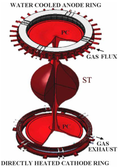
Figure 1.
Schematic of PROTO-SPHERA target configuration, including annular electrodes, centerpost discharge in red color and quasi-spherical toroidal plasma (ST) in brown color.
From fast-camera images, the plasma appears as a linear discharge with variable diameter for a length of about 1 m and takes the shape of a mushroom in front of both annular electrodes (Figure 2), in agreement with magnetic field lines geometry. The plasma region is surrounded by a larger volume filled by neutral gas. The linear part of the discharge is essentially a screw pinch with variable cross-section. The plasma diameter is about 0.5 m at the equatorial plane and decreases to about 0.13 m at the ends of the linear part, consistent with clearance left by two tight-fitting magnetic coils; plasma luminosity sharply drops at field lines that intercept protections of such coils. The main properties of the centerpost plasma are the capability of conducting the desired current within the voltage limits of the power supply and the uniform spreading of current on the anode surface. Such avoidance of anode arc-anchoring is likely due to spontaneous plasma rotation. The line-average density has been measured at the equatorial plane by a second-harmonic laser interferometer [3]. Typical line-average number densities are m and m in Ar and H discharges, respectively. Temperatures in the 2–8 eV range have been found in preliminary Langmuir probe measurements in the mushroom-shaped region. Electric potential measurements are available at the electrodes and at the magnetic coil casings. The voltage drop between the coils at the ends of the linear section gives a rough estimate of the axial electric field, a typical value being 50 V/m. Plasma current and electric potentials are in steady state for most of the plasma duration, which, depending on power supply settings, ranges from 0.3 to 0.8 s.
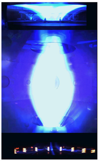
Figure 2.
Image of PROTO-SPHERA plasma in Argon as reconstructed from three cameras, one for the anodic region (top), one for the nearly cylindrical region (middle) and one for the cathode (bottom). View at transitions from linear to mushroom-shaped regions is impeded by coils. The mushroom-shaped plasma is clearly visible in the anodic region at the top. The cathode region appears obscure since sensitivity has been adapted to hot electron emitters (visible as an array of brilliant spots).
A modeling activity is being carried on to help devising optimization strategies and to forecast plasma properties at higher centerpost current. To keep the problem as simple as possible at this preliminary stage, geometrical complexity is neglected and the centerpost plasma is modeled assuming cylindrical symmetry. This approach allows capturing the essential features of plasma dynamics by means of simple calculations and provides useful insights for setting up more realistic models. The purpose of the analysis presented in this work is to evaluate qualitatively (i) the degree of ionization, (ii) the plasma rotation and (iii) the self-generated azimuthal current. The latter could provide a seed for torus formation.
Density measurements and preliminary temperature measurements indicate that mean free paths of plasma particles are much smaller than the plasma size. A fluid description with three interacting species (ions, electrons, and neutral gas) [4,5] has then be adopted. Neutral gas is referred-to as neutrals in the following. The 1-D analysis for ions and electrons is similar to the one developed for magnetized gas discharge plasmas [6,7], but uniform neutral gas density was assumed in those works, while neutral dynamics is kept into account in this work. The effects of decreasing neutral density inside the plasma (neutrals depletion) were reviewed in [8], but without including the confining force that arises from plasma current. On the other hand, screw-pinch analyses including the full electromagnetic force, see for example [9], usually assume fully ionized plasma.
General governing equations are collected in the Appendix A. Simplifying assumptions on which the pinch model is based and the ensuing simple transport equations are presented in Section 2. Numerical results are presented and discussed in Section 3. Conclusions and perspectives are given in Section 4.
2. The Cylindrical Pinch Model
The model for the centerpost plasma is based on some simplifying assumptions which lead to a description in terms of ordinary differential equations. First, the plasma configuration is represented as a cylindrical screw pinch, with negligible flows (excepting axial current) in the axial direction and with constant quantities in both axial and azimuthal directions. This description seems reasonable in the region between the main constrictions shown in Figure 1; no attempt is done to extend the analysis to the mushroom-shaped regions. Second, steady-state condition is assumed, consistent with the experimental observation of flat-top conditions for most of the plasma duration (0.3–0.8 s, with 5 ms initial transient). Third, charge separation is neglected; charged plasma sheaths at plasma-solid interfaces are out of the scope of this work. The model cylindrical plasma is assumed to carry a uniform current density within a radius , which mimics the outer radius of the bright region in Figure 2, which comprises field lines that do not intersect coil protections. The present analysis does not apply beyond such radius, where the plasma flow becomes of the scrape-off type, with substantial axial losses towards solid surfaces. Equations for mass continuity and momentum balance in a mixture of electron, ion and neutral fluids [4,5] are employed. The Argon case is considered, assuming singly charged ions. Energy balance is left out of the present analysis: uniform temperature is assumed and its effect is studied parametrically; modeling energy balance in Ar is a formidable task as it requires accounting for radiation losses from many excited states.
General equations are collected in the Appendix A, while relevant components in cylindrical coordinates are considered in the following subsections. The mixture is described by ion velocity , plasma density n, electric current density , plasma temperature T (assumed common to electrons and ions), neutrals velocity , neutrals density N and neutrals temperature . The z components of velocities are eliminated by the assumption of negligible axial flows. The radial component of current density is eliminated by assumed steady state and 1-D geometry. The other two components are eliminated using Ohm’s law. Plasma temperature is regarded as a parameter and neutrals are assumed to remain at room temperature. Azimuthal components of velocities are eliminated using the respective momentum balances. The radial velocity of neutrals is eliminated by the continuity equation. Three non-linear differential equations for radial ion velocity, plasma density, and neutrals density remain, as detailed in the following subsections. Equations are expressed in SI units for all quantities excepting temperature, which is measured in electronvolts. Final equations are also given in dimensionless form.
The main limitation of this 1-D model is the implication of zero radial current density. The presence of this component, which is possible in 2-D provided that z-dependence and axial return currents preserve charge neutrality, could modify the momentum balance and then it could affect results on azimuthal components of both current density and velocity. On the other hand, 1-D results on the degree of ionization should be exportable to more realistic configurations.
2.1. Mass Continuity
Continuity Equations (A1) and (A2) in steady-state and cylindrical symmetry reduce to
where the plasma number density has been introduced and recombination has been neglected. The ionization rate coefficient in m/s as a function of electron temperature in eV units is [10]
where is the first ionization energy ( 15.76 eV for Ar) and is the electron thermal speed
2.2. Azimuthal Momentum Balance
Model assumptions on cylindrical symmetry and steady state imply radial magnetic field , radial current density , azimuthal electric field and dd. Retaining only dominant rate coefficients, i.e., neglecting when summed with or collision coefficients and neglecting when summed with , the azimuthal component of Ohm’s law takes the form:
where is the electron gyrofrequency and the electron-ion collision rate coefficient is related to e-i collision frequency and to Spitzer resistivity . Constant values of and coefficients are assumed, as listed in Table 1. The azimuthal plasma momentum balance reads

Table 1.
Coefficients for Argon gas (A=40) at room temperature ( eV) from [10] with eV, m, T.
If the electron cyclotron frequency is dominant, i.e.,
then the azimuthal current density takes the simple form
The azimuthal ion velocity is estimated assuming zero net azimuthal momentum
and neglecting convective inertia in (6):
2.3. Radial Momentum Balance
The radial component of plasma momentum balance reads
where the total plasma pressure (temperatures being in eV units) has been introduced and small coefficients have been neglected as in the previous subsection. The term is mainly due to pinch force from the externally imposed plasma current; the plasma pressure it can balance is given by the Bennett relation or its kinetic generalization [11]. The term arises from the self-generated azimuthal current.
The radial component of neutral gas momentum balance reads
2.4. Transport Equations
Equations presented in previous subsections could be closed with energy balance equations [5] accounting for heat transport and radiation. A simpler approach is followed in this work: equations are closed assuming a common constant temperature as a parameter and the character of solutions is studied for different values of the parameter. Neutrals are assumed to remain at room temperature .
From the axial component of Ohm’s law,
uniform electron temperature implies uniform Spitzer resistivity and then nearly uniform , in fact the the last two terms in (12) are negligible, as verified in numerical calculations. The pinch term is then easily calculated:
where is total axial current and R is the pinch outer radius. Centrifugal terms and radial variations of are neglected, as justified a posteriori. Combining (1), (4), (8), (10), (11) and (13) a system of three ordinary differential equations results for plasma density, ions radial velocity, and neutrals density.
where and plasma and neutral gas squared sound speeds have been introduced, and respectively.
A convenient dimensionless form can be obtained introducing the normalized radius , the Mach number and normalized densities and , where is the radial excursion of density in the absence of radial flow (alike to a Bennett pinch).
where is related to slowing of perpendicular diffusion by magnetization, , is related to ion-neutral drag, is a normalized ionization rate, and .
Zeros at the left-hand sides of (17) and (18) correspond to the well-known sonic singularity, which is usually met at plasma-solid interfaces, where it is resolved keeping into account substantial charge separation.
Another important characteristic of the system is introduced by neutrals dynamics. In fact, plasma velocity has a source term proportional to neutrals density, namely the 4th at the RHS of (17). On the other hand, neutrals density can steeply increase with radius since, according to (1), the radial plasma flux (or ) is an increasing function of radius, and then the second term on the RHS of (19) can give rise to super-exponential radial growth. If this happens, the source term in (17) can bring radial velocity to hit the sonic limit.
In practice, since physically acceptable solutions must have no singularities inside the simulation domain, this effect sets an upper limit to the central density of neutrals. The limit changes dramatically with plasma temperature, as discussed in Section 3, the main reason being the strong temperature dependence of the ionization rate coefficient, see Equation (3).
The system is solved in the domain, with boundary conditions at the plasma center , and . The central plasma density is adjusted to fit the measured line-average density (excepting particular cases as detailed in Section 3.1). The central neutrals density is adjusted to have values close to the surrounding gas density, as discussed in next section.
3. Numerical Results
Equations (14)–(16) are solved numerically employing a standard python ode solver. To avoid the geometric singularity at , solutions are advanced starting from a slightly off-axis boundary , with boundary conditions , and . The number density of the surrounding gas is m; the boundary condition on central gas density is adjusted to obtain slightly below . The boundary condition on central plasma density is chosen to reproduce the measured line-average density whenever possible (see next subsection). System parameters are temperature (through , and dependencies), plasma radius (being the pinch force coefficient ), plasma current (being ) and axial magnetic field (being ). Plasma current is fixed at kA. Different values of temperature, plasma radius, and plasma density are considered in the following. Values of the parameters for each case, including the dimensionless ones used in Equations (17)–(19) are listed in Table 2.
Table 2.
Dimensional and dimensionless parameters used in numerical simulations.
3.1. Dependence on Temperature
The plasma radius varies along the pinch axis from 0.27 m to 0.065 and the external magnetic field varies from 0.02 T to 0.6 T; intermediate values of m and T are assumed in this subsection. The character of solutions changes dramatically with temperature; temperature values are chosen in the range 1.0–2.5 eV, which is adequate to capture the different possible regimes.
For eV, the minimum possible , corresponding to has been assumed. The resulting neutrals density varies by less than 20 % across the plasma radius, while the radial profile of plasma density has nearly parabolic shape (Figure 3). The ion radial velocity tends to diverge towards the edge while its value is only times the sonic limit. The reason is the small n at denominator in the first term at the RHS of Equation (14), which arises from finite ion radial flux required in steady state to drain fresh ions produced by ionization. The line-average density is 4.7 × m, i.e., about 20% above the measured value. Lower densities give rise to physically unacceptable solutions as, at this low temperature, plasma pressure becomes insufficient to balance the pinch force and then density decreases to zero inside the simulation domain. The estimated axial electric field is 235 V/m in this case, much higher than the experimental value of about 50 V/m.
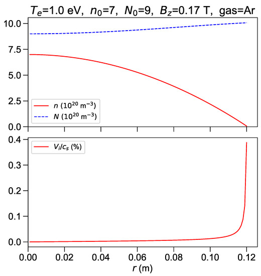
Figure 3.
eV. Upper frame: plasma (solid line) and neutrals (dashed line) number density profiles in m units. Lower frame: ion velocity in percent of the sound speed.
For eV, there is sufficient room to decrease and match the experimental line-average density; the chosen value m corresponds to . At this temperature, neutrals density varies by almost two orders of magnitude from the plasma center to the edge, while the plasma density profile remains parabolic with low edge value (Figure 4). The line-average density fulfills the experimental constraint in this case. Radial velocity tends to diverge towards the edge; the reason is the same as in the 1.0 eV case. The axial electric field is 128 V/m, still substantially higher than the experimental estimate.
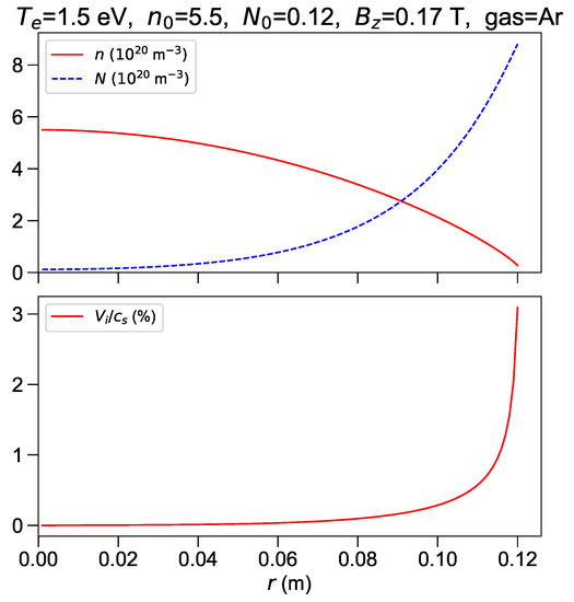
Figure 4.
eV. Upper frame: plasma (solid line) and neutrals (dashed line) number density profiles in m units. Lower frame: ion velocity in percent of the sound speed.
For eV the experimental density is matched with m, which corresponds to . The neutrals density is very small across most of the plasma, and steeply increases in an outer shell (Figure 5). The plasma density profile is flatter than a parabola and the edge value becomes significant. The axial electric field is 83 V/m. Radial velocity steeply increases towards the edge; the reason in this case is not a small denominator but it is the cumulative effect of the source term proportional to neutrals density, as discussed at the end of Section 2.4. Very low is required in this case because the radial growth of neutrals density is steep at this temperature, and with larger the sonic singularity would occur in the simulation domain. The slope of keeps increasing with radius, so the profile cannot smoothly match the outer gas density ; this matching must occur in the scrape-off layer, where field lines intercept coils protections and the radial plasma flow decreases because plasma escapes in the axial direction and recombines at solid surfaces. The scrape-off layer is outside the scope of the present analysis, as discussed above. Profiles at higher temperature are qualitatively similar to the 2.0 eV case, but with flatter plasma density and steeper increase of neutrals density in the outer shell. Results at eV are shown in Figure 6. The estimated axial electric field is 60 V/m in this case, in reasonable agreement with the experimental estimate.
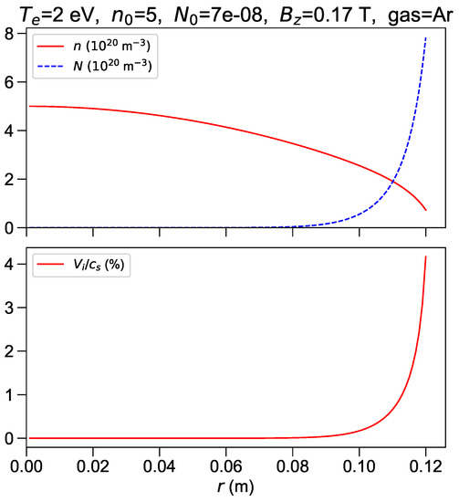
Figure 5.
eV. Upper frame: plasma (solid line) and neutrals (dashed line) number density profiles in m units. Lower frame: ion velocity in percent of the sound speed.
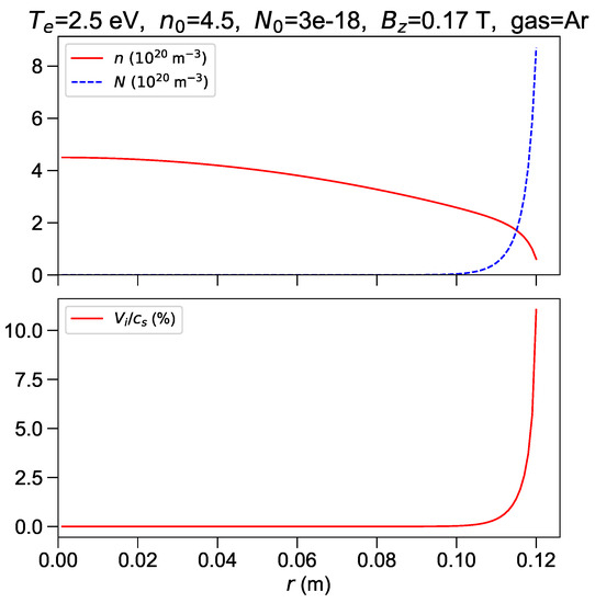
Figure 6.
eV. Upper frame: plasma (solid line) and neutrals (dashed line) number density profiles in m units. Lower frame: ion velocity in percent of the sound speed.
The dramatic change of profiles at eV (far below the 15.76 eV first ionization energy of Ar) is due to reduced neutrals penetration depth. Neutrals penetration is pushed by external gas pressure and contrasted by collisions with outgoing ion flux, which in turn depends on ionization.
The normalized neutrals penetration depth can be estimated from (1) and (19). In dimensionless variables the former reads
Keeping only terms that according to numerical results, are dominant at the plasma edge, in particular the second term at the RHS of (19), one obtains
or
The depth decreases with temperature as strongly increases. At eV, , i.e., there is substantial neutrals density throughout the plasma radius, in agreement with simulations. At 1.5, 2.0 and 2.5 eV one finds 0.51, 0.01 and 0.004, respectively. The last two values are in fair agreement with the relative width across which neutrals density increases from 20 % to 100 % of the edge value. Uniform neutrals temperature has been assumed for simplicity in the model; if neutrals temperature increases inside the plasma, then is to be interpreted as a scale of pressure variation and the scale of density variation becomes even shorter than .
Results on degree of ionization, azimuthal current density from (8) and azimuthal ion velocity from (9) are shown in Figure 7 for the lowest temperature case and in Figure 8 for the highest temperature case. The degree of ionization in the plasma core is 40 % at eV and 100 % at eV, while absolute values of self-generated azimuthal current density and velocity increase substantially at higher temperature.
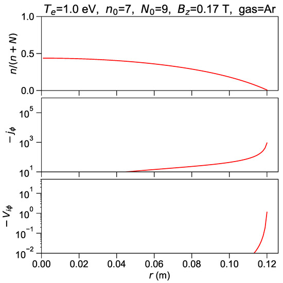
Figure 7.
eV. Upper frame: ionization degree. Intermediate frame: self-generated azimuthal current in A/m. Lower frame: azimuthal ion velocity in m/s.
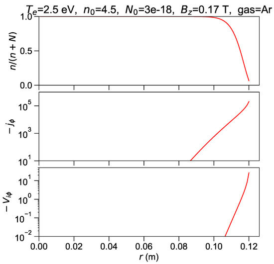
Figure 8.
eV. Upper frame: ionization degree. Intermediate frame: self-generated azimuthal current in A/m. Lower frame: azimuthal ion velocity in m/s.
3.2. Dependence on Plasma Radius and Density
Substantially different profiles are found when changing the plasma radius. Profiles obtained with m (and scaled to preserve magnetic flux) are shown in Figure 9. The ratio between edge and central plasma density (or pressure) is 0.5 in this case, whereas a lower value of 0.14 has been found in the simulation with m (Figure 6). Broadening of density profiles with increasing R is due to lower current density and then to weaker pinch force, total current being fixed. Lower edge density is recovered in simulations at lower central density ( instead of ), as shown in Figure 10. The edge density depends non-linearly on central density, and no acceptable solutions are found (at the chosen radius and temperature) for m.
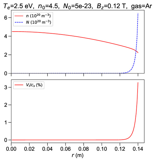
Figure 9.
eV and m. Upper frame: plasma (solid line) and neutrals (dashed line) numer density profiles in m units. Lower frame: ion velocity in percent of the sound speed.
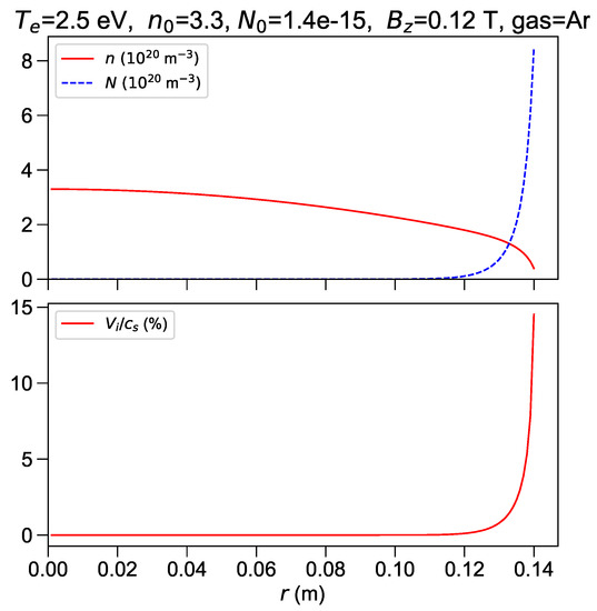
Figure 10.
eV, m and lower density. Upper frame: plasma (solid line) and neutrals (dashed line) numer density profiles in m units. Lower frame: ion velocity in percent of the sound speed.
Consideration of different plasma radii reveals an issue for any future 2D analysis. Envisaging simulations shown in Figure 6 and Figure 9 as representative of different cross sections at different z of the actual pinch, it follows that pressure cannot be constant along field lines, in fact, if it is constant along the field line at the plasma center, then it changes along the field line running at the plasma edge. The reason is that from (13), the pinch force decreases with increasing plasma cross-section. Constant edge density at constant axial density can be restored in the presence of significant azimuthal current density throughout the plasma and not only in the outer region. Driving such current against resistive drag requires radial current , which would be acceptable in 2-D since zero divergence can be preserved by variations of the axial current along z.
However, pressure variations along magnetic field lines remain a relevant issue, in fact the core plasma pressure has to build-up somewhere between the electrodes and the core region. Collisions with neutrals can give at most the pressure of the surrounding gas, which is smaller than the core plasma pressure. Other possible reasons of pressure variation along field lines are pressure anisotropy, inertial forces, and electrostatic forces. The second reason has been invoked in [12] for plasmas with similar local parameters but far from steady state. Electrostatic forces are likely dominant in axial pressure variation close to electrodes. The role of convective inertia and of charge separation will be investigated in future work.
4. Discussion
The model developed in Section 2 allows accounting for three species dynamics with simple and easily controllable calculations. The main result is that owing to the high PROTO-SPHERA densities, the plasma is fully ionized already at eV, well below the Ar first ionization energy. Neutrals penetration is limited to an external layer, in which a substantial radial plasma velocity develops to drain fresh charges produced by ionization. This radial flow across the applied magnetic field drives both azimuthal current and azimuthal ion flow. The latter is a likely cause of the good plasma spreading on the anode surface. The self-generated azimuthal current could be a seed for the formation of a torus encircling the pinch, but this subject requires further work, in particular the uniform assumption should be removed and different applied magnetic fields should be considered, including the presence of x-points, where magnetic reconnection can occur and magnetic flux can be transferred from the pinch to the torus. Another issue that calls for further work is force balance along magnetic field lines, in the presence of the radial pinch force which varies by an order of magnitude in the z direction. Sorting out this item requires consideration of electrostatic and inertial forces, as well as axially resolved diagnostic information on plasma density, temperature, and electrostatic potential.
Author Contributions
Conceptualization, B.T. and P.B.; methodology, B.T. and P.B.; validation, B.T.; experimental data, F.A. and P.M.; writing–original draft preparation, P.B.; writing–review and editing, B.T., F.A. and P.M.
Funding
This research received no external funding.
Conflicts of Interest
The authors declare no conflict of interest.
Appendix A. Mass and Momentum Balance in a Three-Component Plasma
Continuity and momentum balance equations have been adapted from [4,5]. Forms including both time-dependence and charge separation, which could then be used to extend the study to plasma formation phase and to plasma-solid interfaces are presented in this Appendix A, while simplified forms are used in Section 2. Viscosity, pressure anisotropy, and resistivity anisotropy are neglected for simplicity.
Continuity equations for ion number density n, ion velocity , neutral gas number density N and neutral gas velocity read
where and are ionization and recombination rate coefficients, respectively.
Ions, neutral gas, and electrons momentum balance equations read
where , and are ion-neutral, electron-neutral and electron-ion collision rate coefficients respectively; is electron velocity, and are electric and magnetic field respectively, and p denote pressures. Isotropic pressures are assumed. Using more familiar forms result
Introducing charge density and current density , (A8) can be cast as a generalized Ohm’s law
where electron inertia has been neglected. Please note that Spitzer resistivity . Substituting the resistive term from (A9), the ion fluid momentum balance can be cast as
The combination of plasma-neutrals collision coefficients in the second line corresponds to the ambipolar diffusion coefficient of gas discharges with uniform temperature and uniform neutrals density
References
- Alladio, F.; Costa, P.; Mancuso, A.; Micozzi, P.; Papastergiou, S.; Rogier, F. Design of the PROTO-SPHERA experiment and of its first step (MULTI-PINCH). Nucl. Fusion 2006, 46, S613–S624. [Google Scholar] [CrossRef]
- Lampasi, A.; Maffia, G.; Alladio, F.; Boncagni, L.; Causa, F.; Giovannozzi, E.; Grosso, L.A.; Mancuso, A.; Micozzi, P.; Piergotti, V.; et al. Progress of the Plasma Centerpost for the PROTO-SPHERA Spherical Tokamak. Energies 2016, 9, 508. [Google Scholar] [CrossRef]
- Brandi, F.; Giammanco, F. Versatile second-harmonic interferometer with high temporal resolution and high sensitivity based on a continuous-wave Nd:YAG laser. Opt. Lett. 2007, 32, 2327–2329. [Google Scholar] [CrossRef] [PubMed]
- Braginskii, S.I. Transport processes in a plasma. In Reviews of Plasma Physics; Leontovitch, M.A., Ed.; Consultants Bureau: New York, NY, USA, 1965; Volume 1, pp. 205–311. [Google Scholar]
- Meier, E.T.; Shumlak, U. A general nonlinear fluid model for reacting plasma-neutral mixtures. Phys. Plasmas 2012, 19, 072508. [Google Scholar] [CrossRef]
- Sternberg, N.; Godyak, V.; Hoffman, D. Magnetic field effects on gas discharge plasmas. Phys. Plasmas 2006, 13, 063511. [Google Scholar] [CrossRef]
- Allen, J.E.; Holgate, J.T. On the Bohm criterion in the presence of a magnetic field. Nucl. Mater. Energy 2017, 12, 999–1003. [Google Scholar] [CrossRef]
- Fruchtman, A. Neutral gas depletion in low temperature plasma. J. Phys. D Appl. Phys. 2017, 50, 473002. [Google Scholar] [CrossRef]
- Si, X.; Zhao, X. An initial boundary value problem for screw pinches in plasma physics with temperature dependent viscosity coefficients. J. Math. Anal. Appl. 2018, 461, 273–303. [Google Scholar] [CrossRef]
- Lieberman, M.A.; Lichtenberg, A.J. Principles of Plasma Discharges and Materials Processing; Wiley: New York, NY, USA, 2005. [Google Scholar]
- Witalis, E.A. Plasma-physical aspects of charged particles beams. Phys. Rev. A 1981, 24, 2758–2764. [Google Scholar] [CrossRef]
- Kumar, D.; Bellan, P.M. Nonequilibrium Alfvénic Plasma Jets Associated with Spheromak Formation. Phys. Rev. Lett. 2009, 103, 105003. [Google Scholar] [CrossRef] [PubMed]


© 2019 by the authors. Licensee MDPI, Basel, Switzerland. This article is an open access article distributed under the terms and conditions of the Creative Commons Attribution (CC BY) license (http://creativecommons.org/licenses/by/4.0/).