Objective Liutex from Flow Data Measured in a Non-Inertial Frame

Abstract

Objectivity is a fundamental requirement for vortex identification, ensuring that vortex structures observed remain invariant under changes in the reference frame. However, although most conventional vortex identification methods, including Liutex, are Galilean invariant, they are not objective. Since the accelerated motion of the observer does not affect the velocity gradient tensor at an instant of time, the rotational motion is only considered for the non-inertial frame. This paper proposes a method to recover the angular velocity of a rotating observer directly from flow field data measured in the rotating frame. The approach exploits the observation that, in an inertial frame, zero-vorticity points tend to dominate the region with an almost identical nonzero vorticity in the observer’s non-inertial coordinate system. By identifying the most frequently occurring vorticity within the domain, the observer’s angular velocity can be uniquely determined, enabling reconstruction of the objective velocity gradient tensor and, consequently, the objective Liutex. The key issue is to find a reference point (RP). The RP should have zero vorticity in the inertial coordinate system, and then the RP has the same angular speed as the observer. The RP can be found by comparing the vorticity of all points in the computational domain and the RP will correspond to the vorticity vector with the highest percentage in the non-inertial coordinate system. The proposed method is validated using DNS data of the boundary layer transition over a flat plate with an artificially imposed angular velocity. The recovered angular velocity agrees closely with the true value within an acceptable margin of error. Furthermore, the objective Liutex reconstructed from the rotating frame data is visually indistinguishable from the original inertial frame Liutex. These results demonstrate that the method provides a simple and accurate way to restore objectivity for Liutex and other vortex identification techniques. The objective Liutex will be equal to the original Liutex in an inertial coordinate system when the observer does not have rotational motion.

1. Introduction

Vortices are a fundamental element in fluid dynamics research. As stated by Küchemann [1], vortices are the “sinews and muscles of fluid motion”. People’s understanding of vortex definition has gone through three generations [2]. The first-generation identifies vortex by vorticity and vorticity-based methods since vorticity correctly represents the rotation of a rigid body. However, the condition for fluids is different from that for a rigid body as fluids can have shear or stretching. It has been found that vortices can be contaminated by shear [3,4]. Robinson [5] reported a weak correlation between vorticity and vortex in the boundary layer where shear is strong. To overcome the limitations of vorticity-based methods, researchers developed second-generation methods, which rely on the velocity gradient tensor. These methods include the Q criterion [6], ${\lambda }_{ci}$ criterion [7], ${\lambda }_2$ criterion [8], and $\Delta$ criterion [9], among others. While these methods provide better agreement with experimental observations, they still suffer from some common shortcomings. First, these second-generation methods identify vortices by scalar quantities, which do not indicate the orientation of the swirling axis. Second, the physical meaning of the computed values remains unclear. The values provided by these methods do not directly correspond to the angular velocity. In addition, it has been found that the second generation methods can be contaminated by shear or stretching [3,10]. To address these issues, Liutex [11,12], a third-generation method, was proposed. Liutex is a vector quantity with a clear physical interpretation: its direction denotes the swirling axis, and its magnitude equals twice the local angular speed.

Objectivity refers to the property that observed results remain invariant under a change in coordinates. This concept is crucial in the vortex detection, as different researchers may choose different coordinate systems like atmospheric aerial measurement. If the results vary with the choice of coordinates, there would be no consistent standard for comparing the experimental data obtained by different investigators. For example, consider the streamline shown in Figure 1. In the original coordinate system (Figure 1a), the streamline appears as a straight line, and no vortex is visible. However, if the observer is moving at the local streamwise velocity, an evident rotational motion of the flow becomes visible (Figure 1b, locally enlarged in Figure 1c). This illustrates that a non-objective physical concept can be influenced by the change of the frame. Liutex is Galilean invariant [13] and thus remains invariant in different inertial coordinate systems but varies when the coordinate system is non-inertial, such as a rotating frame. Note that Liutex is purely dependent on the $\nabla \mathit{v}$ and the accelerated motion of the frame does not influence the $\nabla \mathit{v}$ since acceleration involves time derivatives, while the $\nabla \mathit{v}$ involves spatial derivatives. This limitation motivates the development of an “objective Liutex” that is independent of the observer’s coordinate system, enabling a coordinate system-free vortex structure.

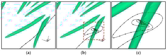
Figure 1. Illustration of the effect of different reference frames on a streamline. (a) A streamline and Liutex isosurface $R=0.07$ in the stationary frame, where no apparent vortex is visible by using streamlines. (b) A streamline and Liutex isosurface $R=0.07$ in a frame moving with the local streamwise velocity, revealing a rotational motion in the red dashed box. (c) Enlarged view of the red boxed region in (b).

To eliminate the ambiguity caused by changes in the reference frame, many researchers have proposed objective vortex identification methods. One natural approach is to determine a distinguished frame of reference, also called as a co-moving or a proper frame [14]. For simple flows, a co-moving frame can be determined properly [15,16,17]. However, finding a proper co-moving frame does not appear feasible for general fluid flows [18]. Some researchers proposed to use the minimal unsteady frame as the proper frame [19,20,21]. Yan et al. [22] proposed to define the proper frame as the one that minimizes the vortex portion. An alternative approach is to introduce a new objective definition of a vortex. Vortex identification methods have been reformulated to their objective forms [23,24,25,26] by subtracting a term, e.g., spatially averaged vorticity, to fully remove the non-objective components in their original definitions. However, this methodology introduces ambiguities into the resulting vortex identification methods since spatially averaged vorticity can be highly dependent on the chosen domain, and the vortex strength obtained through this objective approach is not consistent with its counterpart in the inertial frame. Yu et al. [27] reported an approach to obtain the velocity gradient tensor in an inertial frame from the data measured in a non-inertial frame through a zero-vorticity point. In fact, there is only one point which needs to be found, which is called a “reference point” (RP). However, it lacks a good method to identify such an RP when dealing with black-box data.

Following the study of Yu et al. [27], this paper proposes a simple and practical method to identify the zero-vorticity RP, which constitutes the major contribution of this paper. This approach is based on the observation, which is also used in the research of Yan et al. [22], that strong vortices exist in concentrated regions, while rotations outside these regions are generally weak. Therefore, it is considered that zero-vorticity points tend to occupy most of the space within an inertial frame. If a rotating observer is observing this domain, it will be found that these points occupy most of the space, sharing the same vorticity. Therefore, identifying the zero-vorticity RP in an inertial frame is changed to identifying the largest group of points with a common vorticity in a non-inertial frame. Therefore, any one of these points associated with the most common vorticity can be selected as an RP, and the observer’s angular velocity can be determined from this point.

This paper is organized as follows. Section 2 introduces the concepts of objectivity and Liutex. The method for objective Liutex is presented in Section 3. Section 4 is about the application of this method, and a summary is given in Section 5.

2. Objectivity and Liutex

A tensor field $A\left(\mathit{x},t\right)$ is objective if its corresponding tensor field $\tilde{A}\left(\mathit{y},t\right)$ satisfies [28]

$$\tilde{A}\left(\mathit{y},t\right)=Q^T\left(t\right)A\left(\mathit{x},t\right)Q\left(t\right)$$

(1)

after the Euclidean frame change

$$\mathit{x}=Q\left(t\right)\mathit{y}+b\left(t\right)$$

(2)

where $Q\left(t\right)$ is any rotation tensor and $b\left(t\right)$ is any translation vector.

A vector $\mathit{x}$ is objective if its corresponding vector $\mathit{y}$ satisfies

$$\mathit{x}=Q^T\left(t\right)\mathit{y}$$

(3)

after the Euclidean frame change in Equation (2).

Objectivity means that the measurements of physical quantities are not dependent on the movement of the observer. Regardless of how the observer moves, the measured objective physical quantities remain invariant. Objectivity is particularly important in certain applications, such as atmospheric measurements conducted from a moving aircraft.

The Liutex vector [11] $\mathit{R}=R\mathit{r}$ is defined such that its direction $\mathit{r}$ is the real eigenvector of the velocity gradient tensor satisfying $\mathit{\omega }·\mathit{r}>0$ where $\mathit{\omega }$ denotes the vorticity. The magnitude $R$ can be calculated by [12]

$$R=\mathit{\omega }·\mathit{r}-\sqrt{{\left(\mathit{\omega }·\mathit{r}\right)}^2-4{\lambda }_{ci}^2}$$

(4)

where ${\lambda }_{ci}$ represents the real part of the conjugate complex eigenvalues of the velocity gradient tensor. The direction of the Liutex vector represents the local rotation axis, and its magnitude corresponds to twice the local angular speed.

3. Method for Objective Liutex

Instead of modifying the Liutex definition to an objective version, we aim to find Liutex in an inertial frame. Since Liutex is a Galilean invariant quantity [13], it remains consistent across all inertial frames. Then, the problem is simplified to how to find Liutex in any one inertial frame from the data measured by a non-inertial observer.

Uppercase letters are used to denote variables in the inertial frame while lowercase letters are used to denote variables in the observer’s (non-inertial) frame. Let $X,Y,Z,x,y,z$ be the position components; $\mathit{I},\mathit{J},\mathit{K},\mathit{i},\mathit{j},\mathit{k}$ be the unit basis vectors of the coordinate; $U,V,W,u,v,w$ be velocity components; $\mathit{V},\nabla \mathit{V},\mathit{v},\nabla \mathit{v}$ be velocity vectors and velocity gradient tensors. Suppose that the observer undergoes a translational motion at the velocity of ${\mathit{V}}_t$ (measured in an inertial frame) and a rotational motion at the angular velocity of ${\mathit{V}}_a=V_{ax}\mathit{I}+V_{ay}\mathit{J}+V_{az}\mathit{K}$ (measured in an inertial frame). Note that $\nabla {\mathit{V}}_t=0,$ indicating that the accelerated motion does not influence $\nabla \mathit{V}$. $\nabla \mathit{V}$ and $\nabla \mathit{v}$ have the following relation:

$$\nabla \mathit{V}=T\nabla \mathit{v}{T}^T+\left[\begin{array}{c} 0 -V_{az} V_{ay}\\ V_{az} 0 -V_{ax}\\ -V_{ay} V_{ax} 0\end{array}\right]$$

(5)

where $T$ denotes the transformation matrix from $\mathit{i},\mathit{j},\mathit{k}$ to $\mathit{I},\mathit{J},\mathit{K}$, i.e.,

$$\left[\begin{array}{ccc}\mathit{i}& \mathit{j}& \mathit{k}\end{array}\right]=\left[\begin{array}{ccc}\mathit{I}& \mathit{J}& \mathit{K}\end{array}\right]T$$

(6)

It should be noted that $V_{ax},V_{ay}$, and $V_{az}$ depend only on time $t$, which means that they are uniform throughout the entire space. Thus, if these three values are determined at a single point, they can be applied to the whole domain. $\nabla \mathit{v}$ is the data from the observer and is therefore known. Consequently, $\nabla \mathit{V}$ in the inertial frame can be determined once $V_{ax},V_{ay}$, and $V_{az}$ are obtained at a single point, referred to as an RP. Therefore, the key issue is how to identify such an RP. For simplicity, $T$ is an identity matrix if we let the inertial frame share the same origin and basis vectors as the observer’s frame. In this case,

$$\nabla \mathit{V}=\nabla \mathit{v}+\left[\begin{array}{c} 0 -V_{az} V_{ay}\\ V_{az} 0 -V_{ax}\\ -V_{ay} V_{ax} 0\end{array}\right]$$

(7)

Theorem 1.

If  $\mathit{P}$ is a point of zero vorticity in an inertial frame, which shares the same origin and basis vectors as the observer’s frame, then,

$$V_{ax}=-{\displaystyle \frac{1}{2}}{\omega }_x, V_{ay}=-{\displaystyle \frac{1}{2}}{\omega }_y, V_{az}=-{\displaystyle \frac{1}{2}}{\omega }_z$$

(8)

where ${\omega }_x,{\omega }_y,{\omega }_z$ are the three components of the vorticity at the corresponding $\mathit{p}$ in the observer’s frame

Proof. 

$\nabla \mathit{V}$ can be decomposed into a symmetric part $A$ and a skew-symmetric part $B$.

$$\nabla \mathit{V}=A+B$$

(9)

where

$$A={\displaystyle \frac{1}{2}}\left[\nabla \mathit{V}+{\left(\nabla \mathit{V}\right)}^T\right] B={\displaystyle \frac{1}{2}}\left[\nabla \mathit{V}-{\left(\nabla \mathit{V}\right)}^T\right]$$

(10)

$B$ is a zero matrix since the vorticity is zero at the point $\mathit{P}$. Substitute $\nabla \mathit{V}$ from Equation (5) into Equation (9),

$$A+B=T\nabla \mathit{v}{T}^T+\left[\begin{array}{c} 0 -V_{az} V_{ay}\\ V_{az} 0 -V_{ax}\\ -V_{ay} V_{ax} 0\end{array}\right]$$

(11)

Then, $\nabla \mathit{v}$ can be solved:

$$\nabla \mathit{v}=T^{T}AT-T^T\left[\begin{array}{c} 0 -V_{az} V_{ay}\\ V_{az} 0 -V_{ax}\\ -V_{ay} V_{ax} 0\end{array}\right]T$$

(12)

Here, $T$ is the identity matrix because the chosen inertial frame shares the same origin and basis vectors as the observer’s frame. Thus,

$$\nabla \mathit{v}=A-\left[\begin{array}{c} 0 -V_{az} V_{ay}\\ V_{az} 0 -V_{ax}\\ -V_{ay} V_{ax} 0\end{array}\right]=A+\left[\begin{array}{c} 0 V_{az} -V_{ay}\\ -V_{az} 0 V_{ax}\\ V_{ay} -V_{ax} 0\end{array}\right]$$

(13)

Obviously, $\left[\begin{array}{c} 0 V_{az} -V_{ay}\\ -V_{az} 0 V_{ax}\\ V_{ay} -V_{ax} 0\end{array}\right]$ is the vorticity matrix in the observer’s frame since $A$ is a symmetric matrix. Therefore, $\left(V_{ax}, V_{ay}, V_{az}\right)=-{\displaystyle \frac{1}{2}}\left({\omega }_x,{\omega }_y,{\omega }_z\right)$. Note that the symmetric matrix or strain matrix is objective since Equation (12) indicates that the symmetric matrix of $\nabla \mathit{v}$ is $T^{T}AT$ which satisfies Equation (1). □

Theorem 1 indicates that an RP should have zero vorticity in the inertial frame. It has been found that vortices are in concentrated regions. Yan et al. [22] pointed out that vortex occurrence is highly intermittent in turbulent flows containing numerous vortices. Intense rotational motions are concentrated in localized regions, whereas rotation is generally weak outside these regions. In a direct numerical simulation (DNS) of the flat plate [29], zero-vorticity points are found to occupy 88% of the whole domain. It is intuitive that zero-vorticity regions are likely to occupy the largest area, since the probability that nonzero vorticity vectors take exactly identical values is low. According to Theorem 1, the points that have zero vorticity in the inertial frame correspond to a vorticity of $-2\left(V_{ax}, V_{ay}, V_{az}\right)$ in the observer’s domain. Then, $\left(V_{ax}, V_{ay}, V_{az}\right)$ can be determined by the most frequent occurring vorticity in the observer’s frame. Thus, the RP can be found by comparing the vorticity of all points in the whole computational domain, and the RP will correspond to the vorticity vector with the highest percentage in the observer’s coordinate system.

Based on the discussion above, the procedure to obtain objective Liutex is summarized as follows.

Input: Velocity field data in the observer’s frame. The motion of the observer is unknown.

• Find the RP:

Compute vorticity vectors in the observer’s frame and find the most frequently occurring vorticity vector $\left({\omega }_x,{\omega }_y,{\omega }_z\right)$. For uniform grids, this can be carried out by counting grid points; for non-uniform grids, however, the contribution of each point should be weighted by the associated cell volume. Then, $\left(V_{ax}, V_{ay}, V_{az}\right)=-{\displaystyle \frac{1}{2}}\left({\omega }_x,{\omega }_y,{\omega }_z\right)$.

2.

Compute $\nabla \mathit{V}$ in the inertial frame through Equation (7).

3.

Compute the objective Liutex $\mathit{R}$ from $\nabla \mathit{V}$ as $\nabla \mathit{V}$ is an objective velocity gradient tensor.

4. Numerical Test

We consider a flow over a flat plate [29,30] at Reynolds number $Re={\displaystyle \frac{{\rho }_{\infty }{u}_{\infty }{\delta }_{in}}{{\mu }_{\infty }}}=1000$ where ${\delta }_{in}$ denotes the inflow displacement boundary layer thickness, and $u_{\infty }$ and ${\mu }_{\infty }$ represent free stream velocity and viscosity, respectively. Viscosity is determined by Sutherland’s law in dimensionless form:

$$\mu ={\displaystyle \frac{T^{\frac{3}{2}}\left(1+S\right)}{T+S}}$$

(14)

$$S={\displaystyle \frac{110.3\mathrm{K}}{T_{\infty }}}$$

(15)

where $T_{\infty }=273.15\mathrm{K}$ is the reference temperature. The fluid is Newtonian fluid. This DNS solves Navier–Stokes equations, employing a sixth-order compact scheme for spatial discretization and a third-order Runge–Kutta method for time integration. The Blasius solution, together with two- and three-dimensional Tollmien–Schlichting waves, is imposed at the inlet boundary. Periodic boundary conditions are applied in the spanwise direction, while no-slip conditions are enforced at the wall. Non-reflecting boundary conditions are used at both the outlet and far field boundaries. The dimensions of the computational domain are $L_x=988.658{\delta }_{in}$ (streamwise), $L_y=22{\delta }_{in}$ (spanwise), and $L_{z_{in}}=40{\delta }_{in}$ (wall normal at the inlet). Figure 2 shows the illustration of the computational domain. The $1920\times 128\times 241$ grid points are used in the streamwise, spanwise, and wall normal directions, respectively. The grid is uniformly distributed in the streamwise and spanwise directions, while it is stretched in the normal direction. The first layer thickness at the entrance is found to be 0.43 in wall units ($z^{+}=0.43$). The distance between the leading edge of the flat plate and the upstream boundary of the computational domain is $x_{in}=300.79{\delta }_{in}$. Wall temperature $T_w$ is chosen to be $T_w=273.15\mathrm{K}$.

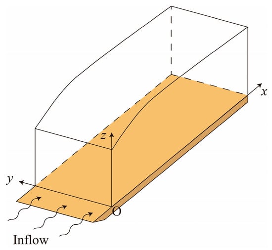
Figure 2. Illustration of the computational domain. The bottom boundary is a flat plate.

Figure 3 shows the visualization of vortex structures, represented by Liutex isosurface $R=0.07$, obtained from the DNS data. Structures of $\mathsf{\Lambda }$ vortices and hairpin vortices, which are typical features in the flow transition, are clearly visible. In Figure 3b, the top view of the vortex structures is presented, showing that in the early stage of the flow transition, the vortex structures still remain symmetrical. Figure 3c shows the side view of the vortex structures. As $x$ increases, the vortex structures grow vertically from the wall and become more complex and irregular, indicating the onset of transition.

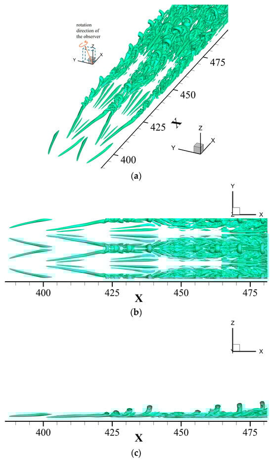
Figure 3. Visualization of vortex structure, represented by Liutex isosurface $R=0.07$, for the DNS of boundary layer transition over a flat plate. (a) Oblique 3D perspective view. (b) Top view. (c) Side view.

An artificial angular velocity ${\mathit{V}}_a=\left(\mathrm{0.1,\; 0.2,\; 0.3}\right)$, as shown in Figure 3a, is applied to generate data from a rotating observer. ${\mathit{V}}_a$ is chosen arbitrarily to test the effectiveness of the proposed method. Figure 4 presents the resulting vortex structures in the rotating reference frame, visualized by the Liutex isosurface $R=0.07$. Compared with the vortex structures in an inertial frame (Figure 3), a notable difference is observed. The symmetry in the early stage totally vanishes and structures of $\mathsf{\Lambda }$ vortices and hairpin vortices become unrecognizable. Overall, the vortex structures appear highly disordered and are severely distorted by the rotating observer. This example clearly shows that regular Liutex is not objective.

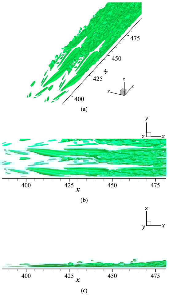
Figure 4. Visualization of vortex structure, represented by Liutex isosurface $R=0.07$, from a rotating observer’s perspective of the DNS of boundary layer transition over a flat plate. (a) Oblique 3D perspective view. (b) Top view. (c) Side view.

The proposed method is effective when dominant vorticity exists within a certain region. So, in practical, the proposed method can be applied to a reduced domain to improve efficiency. In the area defined by the Cartesian product $\left[707, 712\right]\times \left[0, 22\right]\times \left[0, 24\right]$ (blue region in Figure 5), the three vorticities with the highest proportions are listed in Table 1. The vorticity $\left(-0.2056,-0.4027,-0.5938\right)$, which accounts for 39.66%, shows a clear dominance as the second most frequent vorticity accounts for only 1.10%. According to Theorem 1, the corresponding indicated angular velocity of the observer is $(0.1028, 0.20135, 0.2969)$ which is very close to the artificially imposed angular velocity. Table 2 shows that a similar situation occurs in the area $\left[506, 512\right]\times \left[0, 22\right]\times \left[0, 24\right]$ (red region in Figure 5), where the vorticity $\left(-0.2045,-0.4039,-0.6027\right)$ occupies 63.37% and shows an overwhelming lead over the second most common vorticity, which only accounts for 0.83%. The indicated angular velocity is $\left(0.1023, 0.2020, 0.3014\right)$ which is also very close to the artificially imposed angular velocity and within an acceptable margin of error.

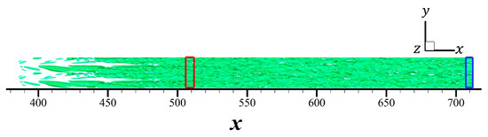
Figure 5. Illustration of the two subdomains used to identify the observer’s angular velocity. Red region represents the area $\left[506, 512\right]\times \left[0, 22\right]\times \left[0, 24\right]$. Blue region represents the area $\left[707, 712\right]\times \left[0, 22\right]\times \left[0, 24\right]$.

Table 1. The three vorticities with the highest proportions in the area $\left[707, 712\right]\times \left[0, 22\right]\times \left[0, 24\right]$.

Vorticity	Percentage
$\left(-0.2056,-0.4027,-0.5938\right)$	39.66%
$\left(-0.1996,-0.3206,-0.4526\right)$	1.10%
$\left(-0.1968,-0.2492,-0.6302\right)$	1.08%

Table 2. The three vorticities with the highest proportions in the area $\left[506, 512\right]\times \left[0, 22\right]\times \left[0, 24\right]$.

Vorticity	Percentage
$\left(-0.2045,-0.4039,-0.6027\right)$	63.37%
$\left(-0.2031,-0.0973,-0.6152\right)$	0.83%
$\left(-0.2010,-0.0477,-0.7084\right)$	0.80%

Theoretically, as long as the subdomain is sufficiently large to yield a dominant vorticity, the identified angular velocity of the observer should be accurate, since the observer’s angular velocity is uniform across the entire domain. In practice, however, some degree of error is unavoidable. Consequently, the angular velocities identified from the previously mentioned two subdomains are close to the true observer angular velocity but exhibit small discrepancies.

After determining the angular velocity of the observer, the velocity gradient tensor in an inertial frame can be obtained by Equation (7) and then the objective Liutex in this inertial frame can be calculated accordingly, which is independent of any non-inertial observer’s frame. Figure 6 shows the Liutex isosurface $R=0.07$ after applying the proposed objective method. Overall, no visible difference is observed between the original vortex structures (Figure 3) and those recovered from the rotating frame data using the proposed objective method (Figure 6). In contrast to Figure 4, Figure 6 preserves the symmetry in the early stage of transition as well as the $\mathsf{\Lambda }$ vortices and hairpin vortices, demonstrating the effectiveness of the proposed method.

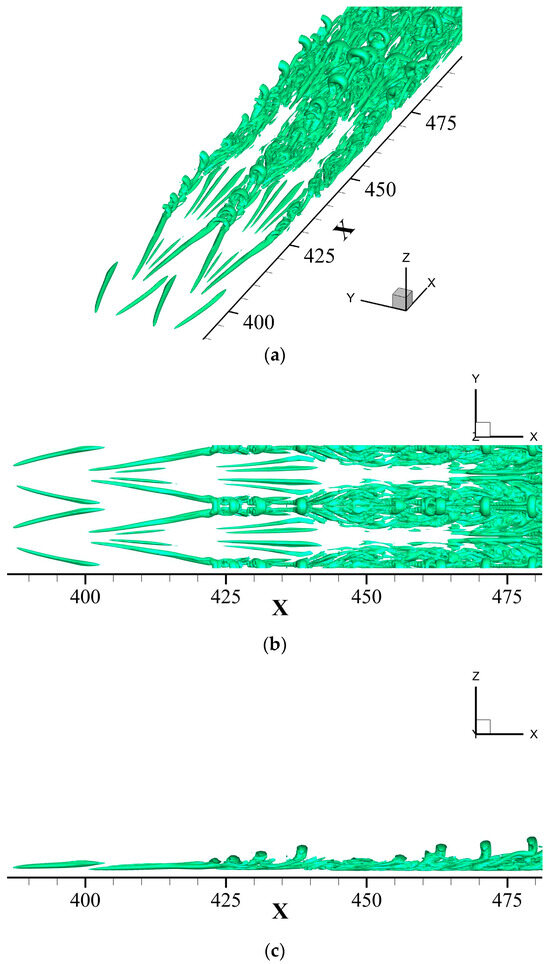
Figure 6. Visualization of vortex structure, represented by Liutex isosurface $R=0.07$, for the DNS of boundary layer transition over a flat plate after implementing the proposed objective method. (a) Oblique 3D perspective view. (b) Top view. (c) Side view.

5. Conclusions

The purpose of this research is to find an objective Liutex for vortex identification and measurement when the observer’s frame is not inertial. The method must be simple to implement and computationally efficient, but very accurate for real measurement like atmospheric aerial measurements. In comparison with other objective methods for vortex in an inertial coordinate system, the proposed objective Liutex by using a reference point is simpler, computationally less expensive, and more accurate.

This paper proposes a method to determine the angular velocity of the observer’s frame using only data measured in that non-inertial frame. By recognizing that zero-vorticity points tend to dominate the region in an inertial frame, the method identifies the most frequently occurring vorticity in the rotating frame and uses it to recover the observer’s angular velocity. Once the observer’s angular velocity is determined, the velocity gradient tensor in the inertial frame can be reconstructed, enabling the computation of objective vortex identification methods such as the objective Liutex.

The proposed method is validated using DNS data of the boundary layer transition over a flat plate with a known, artificially imposed angular velocity. The extracted angular velocity shows excellent agreement with the true values, within an acceptable margin of error. Moreover, the Liutex field reconstructed using the proposed method is visually indistinguishable from the original inertial frame Liutex, demonstrating that the method fully restores objectivity and eliminates contamination caused by the rotating frame.

Overall, the proposed approach provides a simple, efficient, and practical way to achieve objective vortex identification for arbitrary observers. The key idea is to identify the RP that has zero vorticity in the inertial coordinate system and corresponds to the most frequently occurring vorticity value in the non-inertial coordinate system. It can be applied to other vortex identification methods and has potential for use in experimental measurements, numerical simulations, and data-driven flow analysis where observer motion is unknown or difficult to control. Our approach works well for external flow, like flow around a flat plate or airfoil. For more general applications, further validation studies are needed for different flow configurations, such as flow over oscillating airfoils or rotating blades in pumps and turbines.

References

- Küchemann, D. Report on the I.U.T.A.M. Symposium on Concentrated Vortex Motions in Fluids. J. Fluid Mech. 1965, 21, 1. [Google Scholar] [CrossRef]
- Liu, C.; Gao, Y.; Dong, X.; Wang, Y.; Liu, J.; Zhang, Y.; Cai, X.; Gui, N. Third Generation of Vortex Identification Methods: Omega and Liutex/Rortex Based Systems. J. Hydrodyn. 2019, 31, 205–223. [Google Scholar] [CrossRef]
- Shrestha, P.; Nottage, C.; Yu, Y.; Alvarez, O.; Liu, C. Stretching and Shearing Contamination Analysis for Liutex and Other Vortex Identification Methods. Adv. Aerodyn. 2021, 3, 8. [Google Scholar] [CrossRef]
- Yu, Y.; Shrestha, P.; Alvarez, O.; Nottage, C.; Liu, C. Investigation of Correlation between Vorticity, Q, λci, λ2, Δ and Liutex. Comput. Fluids 2021, 225, 104977. [Google Scholar] [CrossRef]
- Robinson, S.K. Coherent Motions in the Turbulent Boundary Layer. Annu. Rev. Fluid Mech. 1991, 23, 601–639. [Google Scholar] [CrossRef]
- Hunt, J.C.; Wray, A.A.; Moin, P. Eddies, Streams, and Convergence Zones in Turbulent Flows. In Center for Turbulence Research Proceedings of the Summer Program; NASA: Washington, DC, USA, 1988. [Google Scholar]
- Zhou, J.; Adrian, R.J.; Balachandar, S.; Kendall, T. Mechanisms for Generating Coherent Packets of Hairpin Vortices in Channel Flow. J. Fluid Mech. 1999, 387, 353–396. [Google Scholar] [CrossRef]
- Jeong, J.; Hussain, F.; Schoppa, W.; Kim, J. Coherent Structures near the Wall in a Turbulent Channel Flow. J. Fluid Mech. 1997, 332, 185–214. [Google Scholar] [CrossRef]
- Chong, M.S.; Perry, A.E.; Cantwell, B.J. A General Classification of Three-Dimensional Flow Fields. Phys. Fluids A Fluid Dyn. 1990, 2, 765–777. [Google Scholar] [CrossRef]
- Kolář, V.; Šístek, J. Stretching Response of Rortex and Other Vortex-Identification Schemes. AIP Adv. 2019, 9, 105025. [Google Scholar] [CrossRef]
- Liu, C.; Gao, Y.; Tian, S.; Dong, X. Rortex—A New Vortex Vector Definition and Vorticity Tensor and Vector Decompositions. Phys. Fluids 2018, 30, 035103. [Google Scholar] [CrossRef]
- Wang, Y.; Gao, Y.; Liu, J.; Liu, C. Explicit Formula for the Liutex Vector and Physical Meaning of Vorticity Based on the Liutex-Shear Decomposition. J. Hydrodyn. 2019, 31, 464–474. [Google Scholar] [CrossRef]
- Wang, Y.; Gao, Y.; Liu, C. Letter: Galilean Invariance of Rortex. Phys. Fluids 2018, 30, 111701. [Google Scholar] [CrossRef]
- Landau, L.D.; Lifshitz, E.M. The Classical Theory of Fields; Butterworth-Heinemann: Oxford, UK, 1975. [Google Scholar]
- Waleffe, F. Exact Coherent Structures in Channel Flow. J. Fluid Mech. 2001, 435, 93–102. [Google Scholar] [CrossRef]
- Mellibovsky, F.; Eckhardt, B. From Travelling Waves to Mild Chaos: A Supercritical Bifurcation Cascade in Pipe Flow. J. Fluid Mech. 2012, 709, 149–190. [Google Scholar] [CrossRef]
- Kreilos, T.; Zammert, S.; Eckhardt, B. Comoving Frames and Symmetry-Related Motions in Parallel Shear Flows. J. Fluid Mech. 2014, 751, 685–697. [Google Scholar] [CrossRef]
- Lugt, H.J. The Dilemma of Defining a Vortex. In Recent Developments in Theoretical and Experimental Fluid Mechanics; Müller, U., Roesner, K.G., Schmidt, B., Eds.; Springer: Berlin/Heidelberg, Germany, 1979; pp. 309–321. ISBN 978-3-642-67222-4. [Google Scholar]
- Rojo, I.B.; Gunther, T. Vector Field Topology of Time-Dependent Flows in a Steady Reference Frame. IEEE Trans. Visual. Comput. Graph. 2019, 26, 280–290. [Google Scholar] [CrossRef]
- Hadwiger, M.; Mlejnek, M.; Theussl, T.; Rautek, P. Time-Dependent Flow Seen through Approximate Observer Killing Fields. IEEE Trans. Visual. Comput. Graph. 2019, 25, 1257–1266. [Google Scholar] [CrossRef]
- Gunther, T.; Theisel, H. Hyper-Objective Vortices. IEEE Trans. Visual. Comput. Graph. 2020, 26, 1532–1547. [Google Scholar] [CrossRef] [PubMed]
- Yan, B.; Wang, Y.; Yu, Y.; Liu, C. New Objective Liutex Vector Based on an Optimization Procedure. Int. J. Heat Fluid Flow 2024, 107, 109407. [Google Scholar] [CrossRef]
- Martins, R.S.; Pereira, A.S.; Mompean, G.; Thais, L.; Thompson, R.L. An Objective Perspective for Classic Flow Classification Criteria. C. R. Mécanique 2016, 344, 52–59. [Google Scholar] [CrossRef]
- Günther, T.; Gross, M.; Theisel, H. Generic Objective Vortices for Flow Visualization. ACM Trans. Graph. 2017, 36, 1–11. [Google Scholar] [CrossRef]
- Liu, J.; Gao, Y.; Liu, C. An Objective Version of the Rortex Vector for Vortex Identification. Phys. Fluids 2019, 31, 065112. [Google Scholar] [CrossRef]
- Liu, J.; Gao, Y.; Wang, Y.; Liu, C. Objective Omega Vortex Identification Method. J. Hydrodyn. 2019, 31, 455–463. [Google Scholar] [CrossRef]
- Yu, Y.; Wang, Y.; Liu, C. A Letter for Objective Liutex. J. Hydrodyn. 2022, 34, 965–969. [Google Scholar] [CrossRef]
- Gurtin, M.E. An Introduction to Continuum Mechanics; Mathematics in Science and Engineering; Academic Press: New York, NY, USA, 1981; ISBN 978-0-08-091849-5. [Google Scholar]
- Wang, Y.; Yang, Y.; Yang, G.; Liu, C. DNS Study on Vortex and Vorticity in Late Boundary Layer Transition. Commun. Comput. Phys. 2017, 22, 441–459. [Google Scholar] [CrossRef]
- Chen, L.; Liu, X.; Oliveira, M.; Liu, C. DNS for Late Stage Structure of Flow Transition on a Flat-Plate Boundary Layer. In Proceedings of the 48th AIAA Aerospace Sciences Meeting Including the New Horizons Forum and Aerospace Exposition, Orlando, FL, USA, 4–7 January 2010; American Institute of Aeronautics and Astronautics: Orlando, FL, USA, 2010. [Google Scholar]
Disclaimer/Publisher’s Note: The statements, opinions and data contained in all publications are solely those of the individual author(s) and contributor(s) and not of MDPI and/or the editor(s). MDPI and/or the editor(s) disclaim responsibility for any injury to people or property resulting from any ideas, methods, instructions or products referred to in the content. |
© 2025 by the authors. Licensee MDPI, Basel, Switzerland. This article is an open access article distributed under the terms and conditions of the Creative Commons Attribution (CC BY) license.