An Image-Based Technique for Measuring Velocity and Shape of Air Bubbles in Two-Phase Vertical Bubbly Flows

Abstract

Bubbly flow is a flow regime common in many industrial applications involving heat and mass transfer, such as reactors, cooling systems, and separation units. Accurate knowledge of bubble velocity, shape, and volume is crucial as these parameters directly influence the efficiency of phase interaction and the mixing process performance. Over the past few decades, numerous techniques have been developed to measure the velocity, shape, and volume of bubbles. Most efforts have focused on non-intrusive methods to minimize disturbance to the flow. However, a technique capable of simultaneously measuring these bubble characteristics across a dense spatial domain remains elusive. In this research, an image-based technique that enables simultaneous measurement of bubble velocity, shape, and volume in bubbly flows over a densely sampled linear domain is presented. A high-speed camera captures the variation in light intensity as bubbles pass in front of a collimated laser sheet, providing real-time, high-resolution data. The accuracy of the proposed methodology is evaluated and the uncertainties associated with the velocity and volume measurements are quantified. Given the promising results and the simplicity of the hardware and setup, this study represents an important step toward developing a technique for online monitoring of industrial processes involving bubbly flows.

1. Introduction

Two-phase gas–liquid flows are prevalent flow regimes in a wide range of industrial applications, from oil and gas extraction to metal production and nuclear power plants [1,2]. Among these, bubbly flows represent a specific flow pattern where discrete gas bubbles are dispersed within a continuous liquid phase [3,4]. Bubbly flow regime typically occurs at relatively low gas flow rates, leading to the formation of small, spherical or near-spherical bubbles that are generally evenly distributed throughout the liquid [5]. Optimizing processes involving bubbly flows is critical for enhancing the interfacial surface area between the gas and liquid phases, which directly improves heat and mass transfer rates [6,7]. The complex interaction between the two phases pose significant challenges for both numerical modeling [8,9,10] and experimental investigation [11,12,13]. Nevertheless, the low uncertainty characterization of two-phase flows is crucial for improving the performance of key industrial systems, including fluidized bed reactors, cooling mechanisms, and separation processes [14,15,16].

Typically, dedicated sensors are installed inside pipes, making direct contact with the flow [17,18,19]. More recent approaches, however, have focused on non-intrusive techniques using ultrasonic or thermal waves [20,21,22]. Although these methods reduce measures and modifications, they still provide sparse or averaged measurements across the pipe’s cross-section. Imaging techniques offer a solution to this limitation by allowing for the acquisition of dense data. Particle Image Velocimetry (PIV) and Particle Tracking Velocimetry (PTV) [15,23,24] are well-established full-field methods used to measure velocity fields in fluid mechanics. Additionally, for multi-phase flows, several techniques employ tomographic methods to map the phase distributions across a pipe section [25,26,27,28,29]. Other methods rely on the interaction between the phases and light at various wavelengths [30,31]. Specifically, the presence of air bubbles within the optical path alters how light is transmitted through the liquid phase. By measuring light intensity using photoelectric transducers, this interaction can be analyzed. With the development of such electronic components, various measurement techniques based on light–fluid interactions have been proposed and explored. For instance, Liu et al. [32] investigated the characteristics of film bubbles, including their size, shape, and axial and radial distributions, using planar laser-induced fluorescent light. Similarly, Xue et al. [33] proposed a method to reconstruct bubbly plumes by using a high-speed camera to capture slicing images, obtained by sequentially scanning the flow with a laser sheet. Mithran et al. [34] developed and experimentally validated a numerical model to predict the irradiation behavior of infrared rays when interacting with bubbles of different sizes. A technique proposed by Guet et al. [35] employs a fiber optic probe to simultaneously measure both bubble size and velocity. While fiber optic probes are commonly used in industrial multiphase reactors [36], they typically only provide pointwise measurements [37,38]. To the best of the authors’ knowledge, no current study on bubbly flows presents a technique for simultaneously measuring both the shape and the velocity of bubbles in a dense spatial domain. Moreover, by determining the shape of the bubbles, its volume can also be estimated, allowing for the estimation of the quantity of air that is flowing through a given section of a pipe.

This paper introduces a methodology that extends the fiber-optic-probe approach, enabling the characterization of a bubbly plume in a linear spatial domain with enhanced resolution compared to the point-based techniques. The proposed method is based on the principle that the intensity of a coherent light source, specifically a green laser sheet, passing through a transparent tank, is proportional to the air–liquid phase distribution within the tank’s cross-section. To reconstruct the shape of bubbles rising through the water column, two horizontal lines of pixels from the entire CCD camera matrix are analyzed. The accuracy of this algorithm was validated via a comparison with reference data on bubble velocity and volume. The technique was further tested in a real-world scenario, where a known volume of air was injected into a water tank to create a rising bubbly plume. A key advantage of this technique is its minimal need for parameter adjustments, making it highly suitable for online monitoring of industrial bubbly flows.

The manuscript is organized as follows. In Section 2, the basic principle and hypotheses were outlined, before illustrating the method step by step. In Section 3, the measurement setup and the experimental protocol are described in detail. In Section 4, the results of the experimental campaigns are shown and discussed. Section 5 draws the conclusions.

2. Methodology

The proposed methodology is based on two fundamental principles. The first principle is that an air bubble behaves optically like an opaque object, transmitting only a fraction of the light that hits it. As a result, when a bubble travels in front of a light source, it creates a region of light attenuation that mirrors the bubble’s shape. By capturing the variation in light intensity over time along an interrogation line (IL), the shape of the bubble as it crosses can be measured. The second principle involves constructing an image by stacking light intensity data over time. The resulting image represents the system in a Space–Time domain (STd), where the x-axis corresponds to the array of photo-detectors, and the y-axis represents the bubble traveling time. In this domain, bubbles appear as “blobs”. By analyzing the blobs in the STd, the crossing velocity of the bubbles can be determined. This velocity is crucial for converting the blob shape in the STd into the actual shape of the bubble, which exists in the Space–Space domain (SSd). It is important to note that the x-axis remains the same in both the STd and SSd.

The proposed technique requires several assumptions to be satisfied as the bubble travels between two interrogation lines of pixels in the CCD camera sensor: the bubble’s motion can be approximated by its vertical displacement; the bubble’s shape is assumed to remain constant while transiting on the two ILs; and the bubble is considered to have the shape of an oblate ellipsoid. To ensure the validity of the two assumptions, the two ILs are placed very close to each other. In this way, the displacement can be considered strictly vertical and the shape can be expected to remain the same, even in the presence of solid particular matter diluted within the fluid. Also, Besagni et al. [11,12] experimentally demonstrated the validity of these assumptions when the measurement is performed far from the point of air injection, in regions where the flow is well developed and free from bubble coalescence or breakup phenomena. They also showed that smaller, spherical bubbles tend to rise more vertically, further supporting these assumptions. The third assumption is supported by many theoretical and experimental studies [8,12,13] that discussed how the bubble shape is completely defined by knowledge of its major and minor diameters.

Figure 1 illustrates the working principle of the proposed method, where two lines of pixels are used as interrogation lines (ILs), and a green laser sheet serves as the coherent light source. From these two ILs, two Space–Space domain (SSd) images are generated. As the bubble’s velocity is essential for reconstructing its shape and calculating its volume, the first step is to track and match the same bubble in both SSd images.

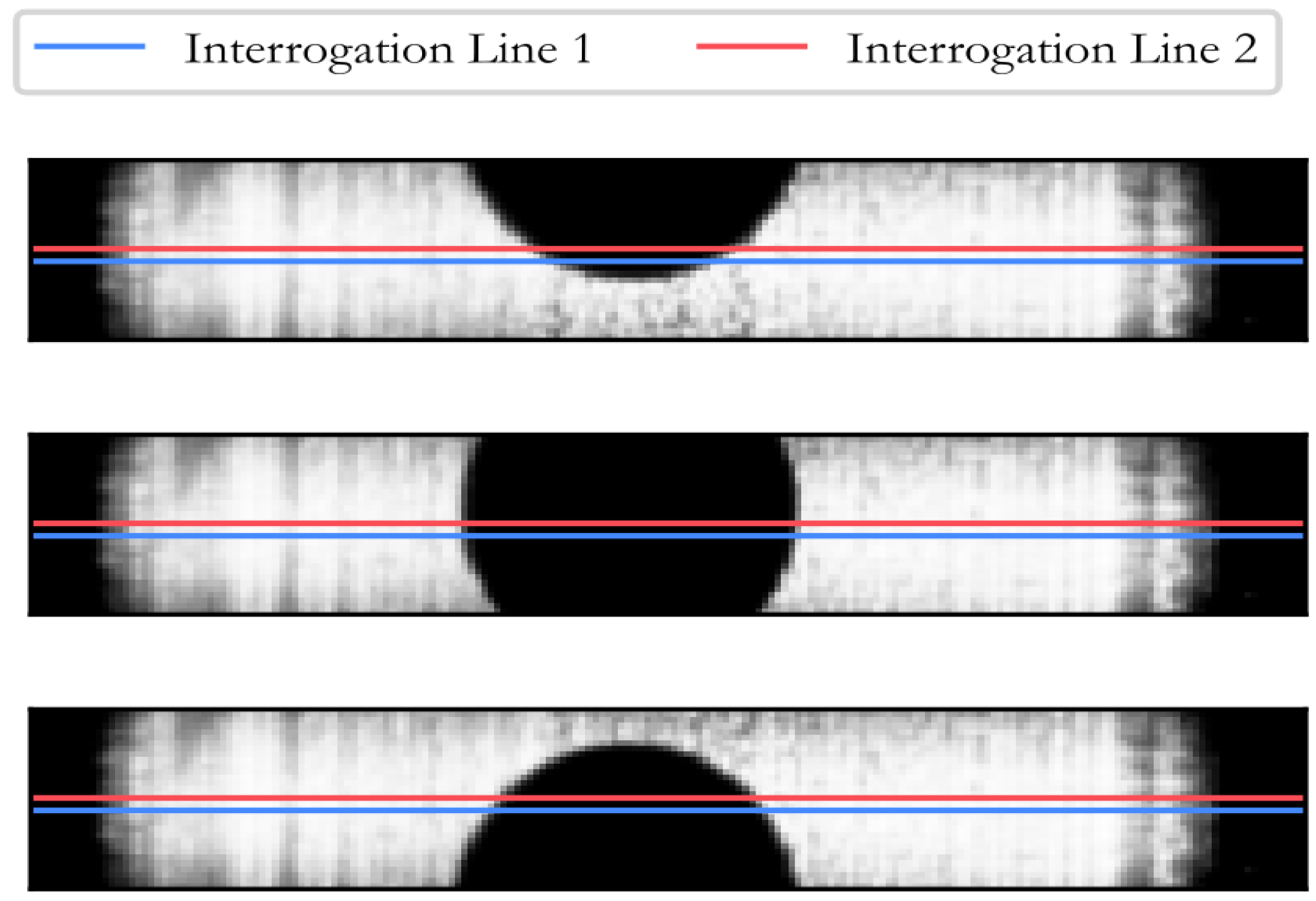
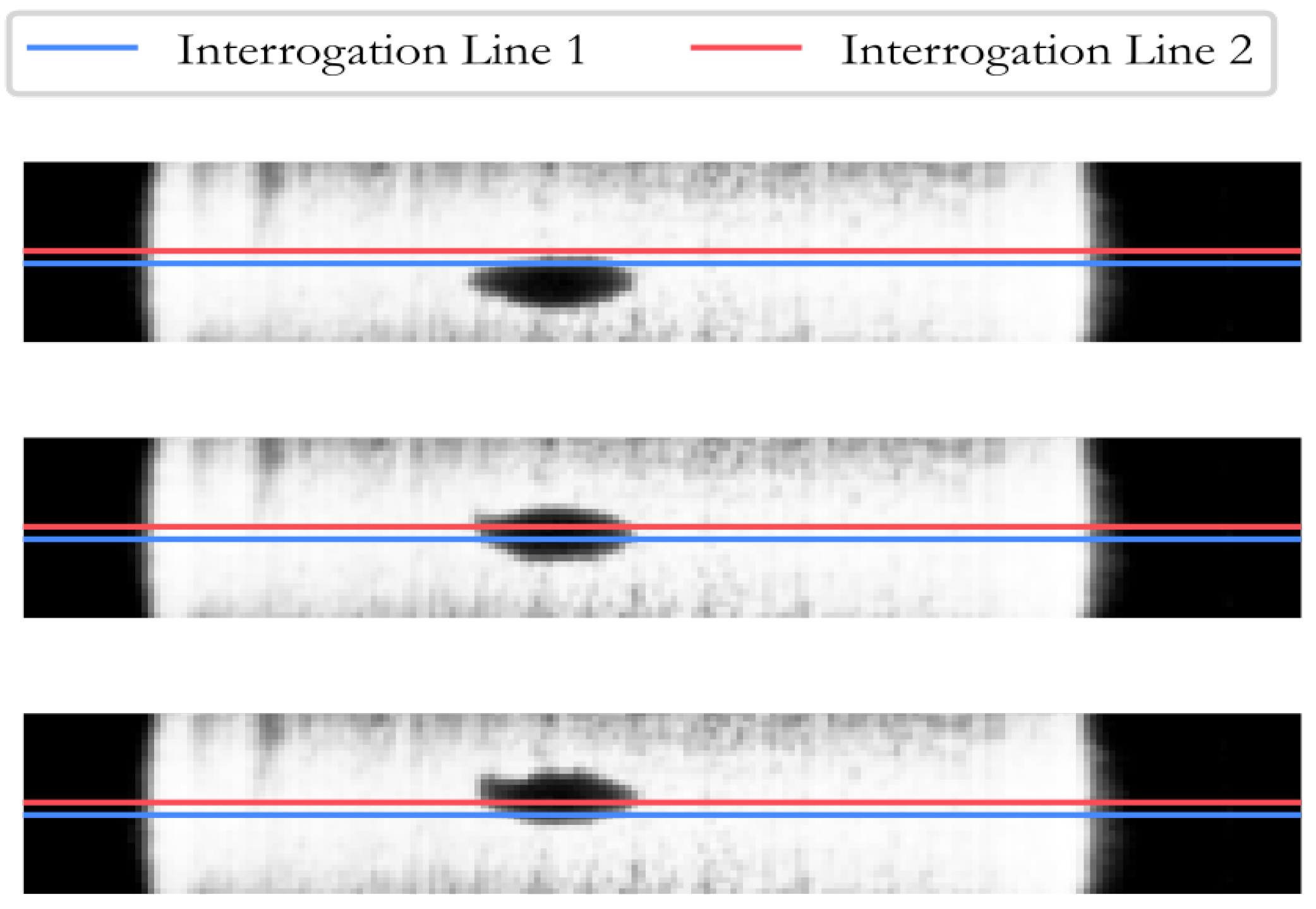
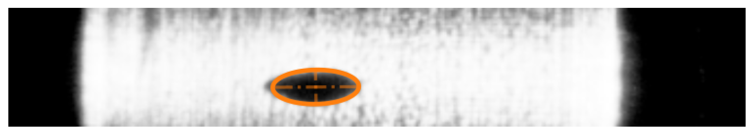
2.1. Bubble Matching

Stacking the light intensity data acquired along the two ILs (see Figure 1), generates two representations in the STd shown in Figure 2. Light that reaches the IL depends on the bubble section that is transiting in front of the IL in that instant. To obtain the blob shape that corresponds to the bubble in Figure 2, a threshold was set on light intensity, so that each point of the blob has the same value.

The crossing of multiple bubbles during a single acquisition results in multiple blobs appearing within the same representation. To determine the velocity of each bubble, it is essential to correctly identify the same blob in both representations. A robust and efficient method for recognizing and matching the same bubble is achieved using the Jaccard similarity coefficient, also known as the Intersection over Union (IoU) index [39]. The IoU is defined as the ratio of the area of intersection to the area of union between two shapes. For two contours, A and B, the IoU is calculated as

$$\mathrm{IoU}={\displaystyle \frac{|A\cap B|}{|A\cup B|}}.$$

(1)

The contour of each blob is extracted, producing two sets of contours, one corresponding to the bubbles as they cross IL1, and the other as they cross IL2. The second key assumption (i.e., the bubble’s deformation is negligible between the two ILs) implies that the same bubble will have identical contour in both images. To match a bubble in the IL1 representation, the IoU index is computed between its own contour and all the contours in the IL2 representation. The contour with the highest IoU value is identified as the corresponding bubble. This allows for the measurement of the velocity and volume of each bubble individually.

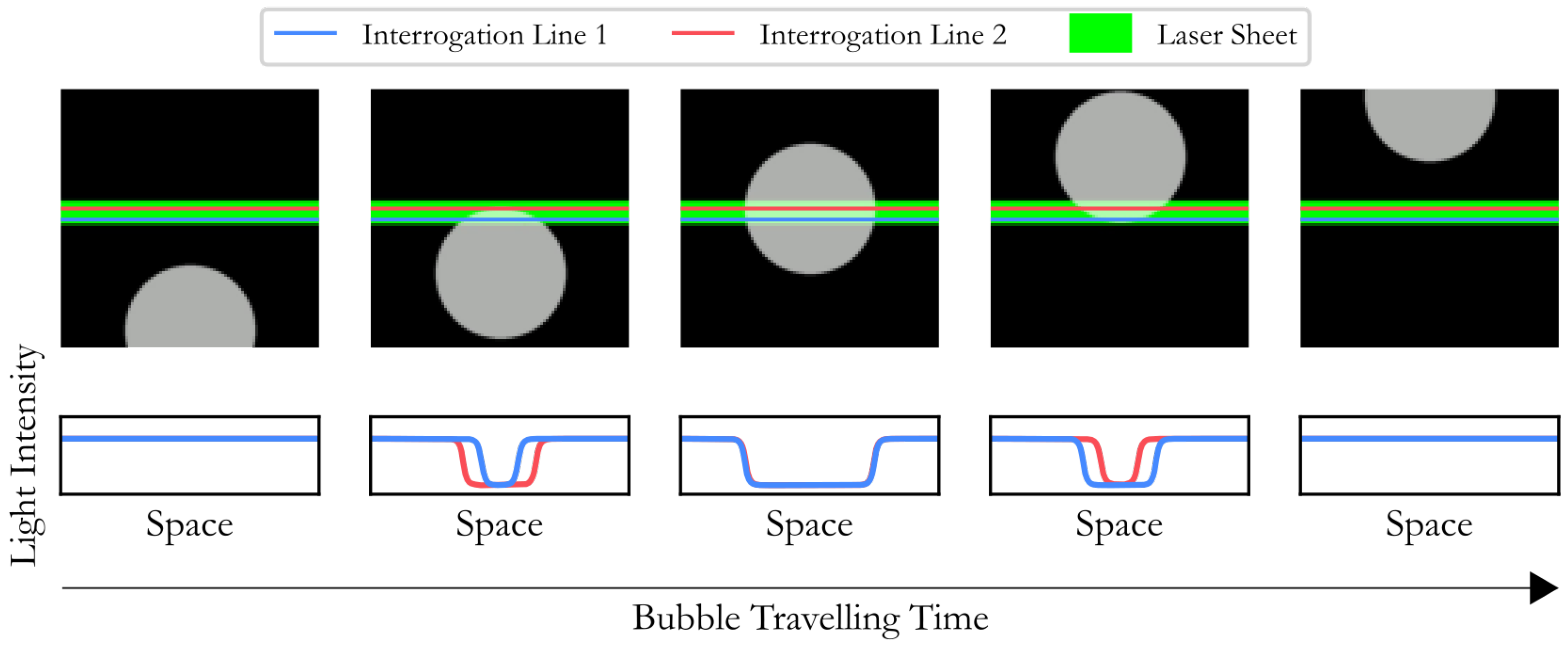
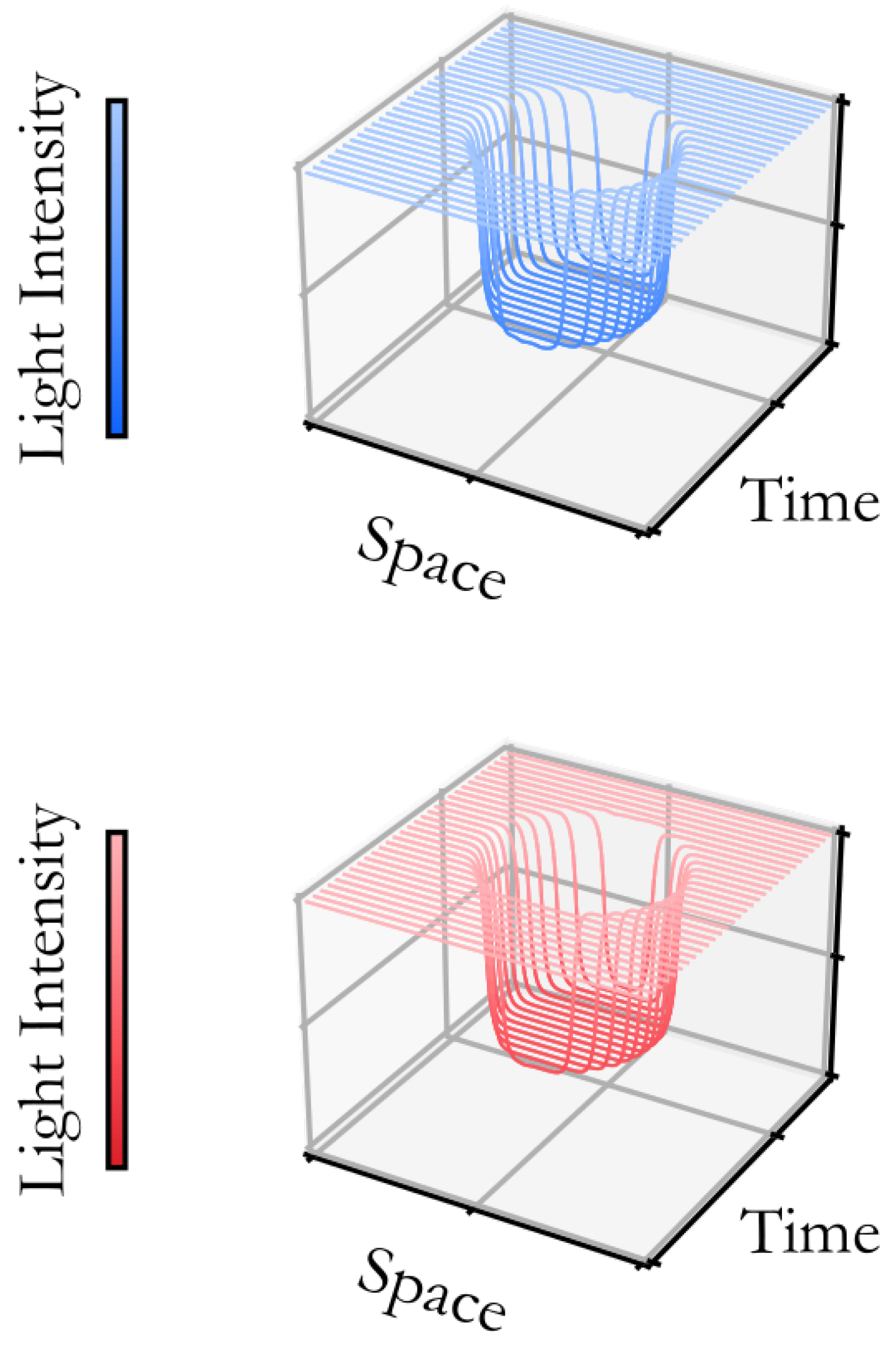
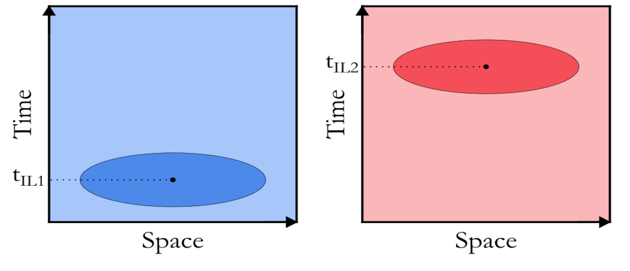
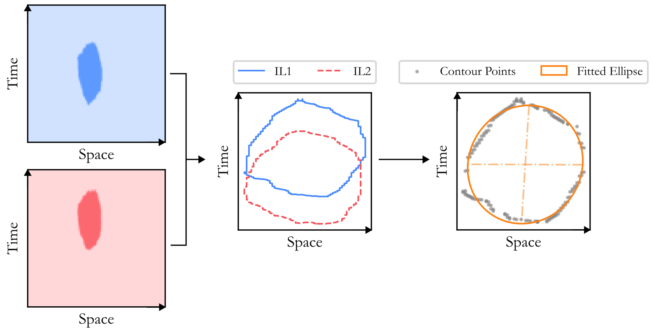
2.2. Measuring the Velocity of the Bubble

Once each bubble is isolated, the next step consists of calculating the x- an y-coordinates of centroids of the two contours as the ratios between the image moments [40] of these two regions (see Figure 3). As these are coordinates in the STd, it is possible to measure the time $\Delta t$ needed for the bubble to move from IL1 to IL2 by computing the difference between the two y-coordinates of the centroids. The velocity is then obtained as the ratio between the known distance between the two ILs ($\Delta s$) and $\Delta t$.

Once each bubble is isolated, the next step (Figure 3) involves calculating the x- and y-coordinates of the centroids of the two contours, which are determined as the ratios of the image moments of these regions [40]. Since these coordinates are in the STd, the time interval $\Delta t$ required for the bubble to travel from IL1 to IL2 can be measured by calculating the difference between the y-coordinates of the centroids. The bubble’s velocity is then obtained by dividing the known distance between the two ILs ($\Delta s$) by $\Delta t$:

$$v={\displaystyle \frac{\Delta s}{\Delta t}}$$

(2)

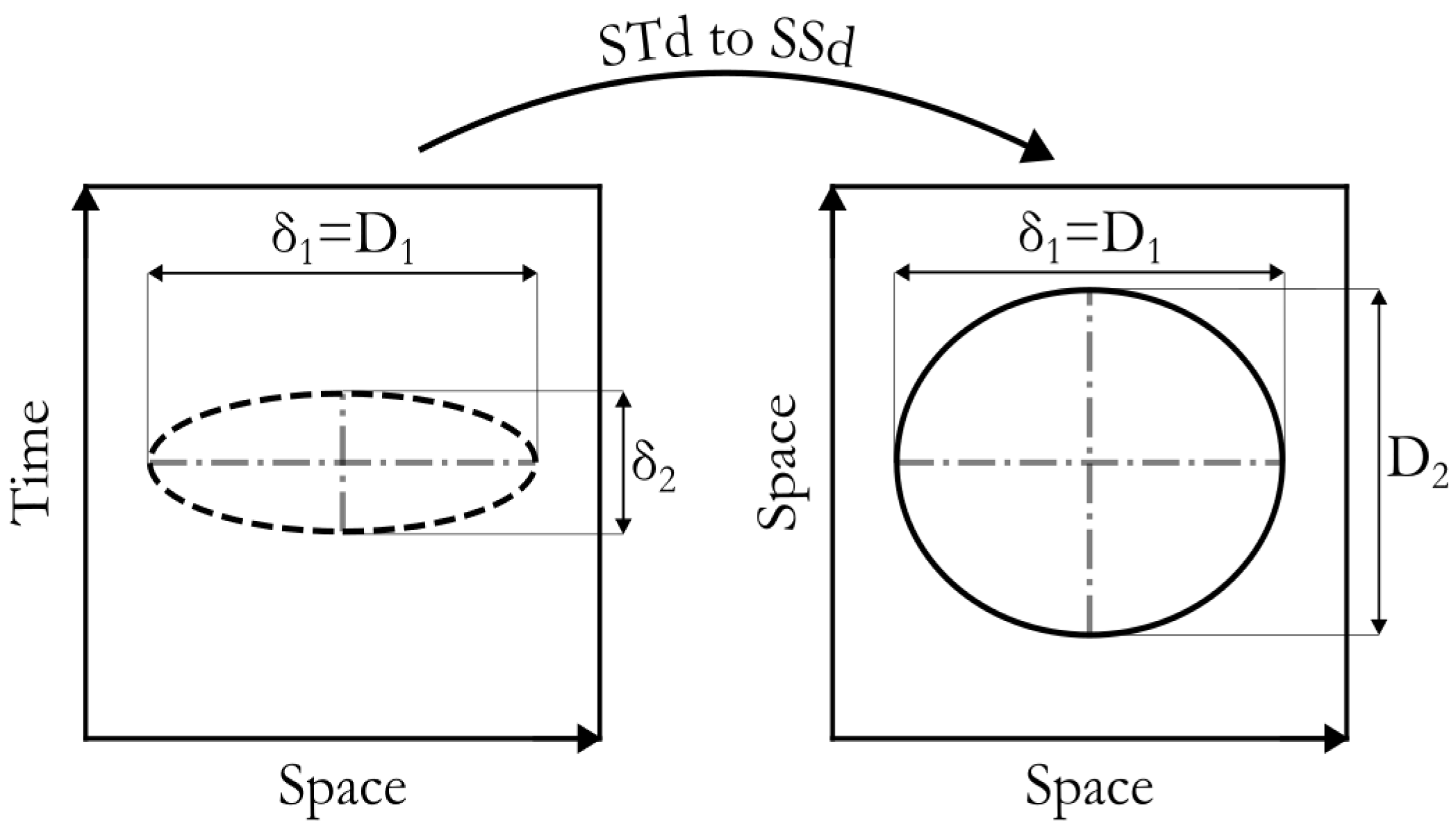
2.3. Reconstructing Shape and Volume of the Bubble

To calculate the bubble’s volume, the third assumption is used (i.e., the bubble can be approximated as an oblate ellipsoid). An ellipse is fitted to the contour points of the blob in the STd. A transformation is then required to map this ellipse to the SSd, where the diameters of the ellipse represent the effective dimensions of the bubble. As discussed in Section 2, the x-axis is the same in both domains and it aligns with the IL on the CCD, so the diameter of the bubble along this axis remains unchanged. However, the diameter perpendicular to this axis must be scaled from the time domain to the space domain. The scaling factor is the bubble’s rising velocity. The transformation can be observed in Figure 4.

This transformation is valid if the angle between the horizontal axis and a diameter of the ellipse is close to zero. In practice, a bubble rising freely in a steady-water column tends to become flattened due to the pressure gradient. As the bubble rises and reaches a stable shape, the vorticity of the surrounding liquid creates a wake beneath the bubble [9,10]. The assumption of negligible tilt was experimentally validated by measuring the tilting angle of the fitted ellipses.

3. Materials and Methods

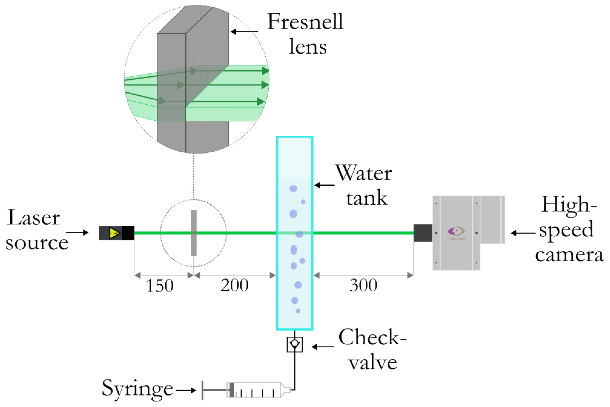
3.1. Measurement Setup

The experimental campaign was conducted using a 50 mm × 50 mm × 390 mm acrylic glass container filled with water to a height of 270 mm (±0.5 mm). A check valve was installed at the bottom of the container to prevent water from spilling out when no air was injected. A laser sheet was projected at a height of 240 mm (±0.5 mm) from the bottom of the tank using a 50 mW, 532 nm laser module with a 120° beam angle. This distance from the injection point guaranteed the avoidance of bubble coalescence and breakup phenomena. In the presence of an opaque object, the divergent laser rays produced a light attenuation area in the CCD, scaled based on the relative distance between the laser and the object. To prevent this distortion, a 75 mm × 75 mm Fresnel lens was used to collimate the laser sheet, ensuring that the dimensions of the attenuation area remained constant regardless of the object’s position. By positioning the laser module at the focal length of the Fresnel lens (150 mm), the resulting beams were parallel. The Fresnel lens was placed 200 mm from the tank. A PHANTOM VEO E310-L high-speed camera (Vision Research, Wayne, New Jersey, USA), coupled with a 50 mm f/1.8D AF Nikkor lens, was used to record the experiment. The camera, positioned 300 mm from the tank, captured video at a resolution of 442 × 60 pixels, with a frame rate of 20 kHz. This setup provided a spatial resolution of 0.125 mm/pixel in both dimensions. The distance between the ILs was set at 14 pixels, corresponding to 1.75 mm. To inject a known volume of air into the system, a 60 ml syringe was used as a reference for volume measurements. A schematic representation of the experimental setup is shown in Figure 5.

3.2. Experimental Campaign

To evaluate the metrological performance of the algorithm, reference values for both velocity and volume were necessary. A metallic sphere with a diameter of 15 ± 0.5 mm was dropped from the top of the empty tank. Assuming negligible air resistance, the falling speed was calculated using the following equation:

$$v=\sqrt{2gh},$$

(3)

where h is the distance between the top of the tank and the impact location (150 ± 0.5 mm), and g is the gravitational acceleration. Since the sphere is a rigid body falling vertically, the first two assumptions outlined in Section 2 are then satisfied. The uncertainty in distance measurements propagates into the uncertainty in velocity, which can be calculated from Equation (3) as [41]

$$u\left(v\right)=\left({\displaystyle \frac{\partial v}{\partial h}}\right)·u\left(h\right)=0.006\mathrm{m}/\mathrm{s}.$$

(4)

Rather than using the shape of the sphere as a reference, its volume was calculated and used for the metrological assessment. A total of five tests were conducted, with the sphere dropped from the same height in each case. Here, the uncertainty in volume is calculated as [41]

$$u\left(V\right)={\displaystyle \frac{\partial V}{\partial r}}·u\left(r\right)={\displaystyle \frac{\partial \left(\frac{4}{3}\pi r^3\right)}{\partial r}}·u\left(r\right)=0.3{\mathrm{mm}}^3.$$

(5)

The algorithm was subsequently applied to air bubbles. Although no reference was available for the increasing velocity of the bubbles, a syringe was used to inject 5 mL of air into the tank.

Furthermore, the impact on volume due to the pressure exerted by the water column above the air bubbles as they cross the laser can be determined using Stevin’s Law:

$$\Delta P=\rho gl=0.294\mathrm{kPa},$$

(6)

where $\rho$ denotes the density of water and l represents the distance between the elevation of the water’s free surface and the laser sheet (30 mm). Given that this $\Delta P$ is less than 1% relative to atmospheric pressure, this effect can be neglected. As a result, the volume measured by the syringe served as the reference for measuring the cumulative volume of the resulting bubbles. It also enabled the evaluation of the assumptions made in the measurement process. This test was repeated three times.

4. Results and Discussions

4.1. Reference on Velocity and Volume

Using the acquisition parameters listed in Section 3.1, the video of the sphere falling was acquired and repeated five times. In Figure 6, a few frames from one of the acquisitions are shown.

Listed in

Table 1. Results of the measurements on diameters, velocity, and volume of the free-falling sphere.

	${\mathit{D}}_1$ [mm]	${\mathit{D}}_2$ [mm]	V$\left[{\mathrm{mm}}^3\right]$	v [m/s]
Test 1	14.658	14.710	1660.8	1.786
Test 2	15.014	14.687	1733.4	1.786
Test 3	15.170	14.681	1768.9	1.786
Test 4	15.264	14.628	1784.6	1.786
Test 5	14.858	14.754	1705.4	1.786
$\mu$	14.993	14.692	1730.6	1.786
$\sigma$	0.21	0.04	44.6	0.000
REF	15	15	1767	1.715
u (REF)	0.005	0.005	0.3	0.006
$\overline{ϵ}$ [%]	1.24	2.05	2.5	4.09

are the results of the method applied to the real videos. Here, the volume V was calculated by considering the reference sphere as an oblate ellipsoid. The resulting $\overline{ϵ}$ is the mean percentage deviation of the measured value with respect to the reference.

The standard uncertainty in velocity and volume, $u\left(\mathit{v}\right)$ and $u\left(V\right)$, respectively, are calculated from the corresponding standard deviations as follows [41]:

$$u\left(v\right)=\sqrt{{\displaystyle \frac{{\displaystyle \sum _i^5}{(v_i-\overline{v})}^2}{n-1}}}=\sigma \left(v\right)=0\mathrm{m}/\mathrm{s},$$

(7)

$$u\left(V\right)=\sqrt{{\displaystyle \frac{{\displaystyle \sum _i^5}{(V_i-\overline{V})}^2}{n-1}}}=\sigma \left(V\right)=44.6{\mathrm{mm}}^3.$$

(8)

Also, the uncertainties due to the repeatability of the measurement were calculated:

$$u_r\left(\overline{v}\right)={\displaystyle \frac{u\left(v\right)}{\sqrt{n}}}=0\mathrm{m}/\mathrm{s},$$

(9)

$$u_r\left(\overline{V}\right)={\displaystyle \frac{u\left(V\right)}{\sqrt{n}}}=25.70{\mathrm{mm}}^3,$$

(10)

where n is the number of tests conducted, and $\overline{V}$ and $\overline{v}$ are the mean volume and velocity over the five tests.

Despite the $4.09\%$ bias ($\overline{ϵ}$), the the null dispersion on v shows how high the precision of the algorithm is when measuring velocity. This bias also influences the reconstruction of the diameter $D_2$, which affects the measurement of the volume of the sphere. Also, the reconstruction of both diameters suffers from the low spatial resolution of the acquisition. In addition, given the fixed focal length of the lens used and the necessity of high frequencies, the laser sheet covers only a fraction of the 442 pixels of the ILs (Figure 6).

4.2. Application on Bubbly Flow

Maintaining the acquisition parameters listed in Section 3.1, 5 mL of air was injected in the tank filled with water. In Figure 7, some frames of one real bubble rising in the water tank are shown.

Following Section 2.1, the light attenuation profiles from ${\mathrm{IL}}_1$ and ${\mathrm{IL}}_2$ over time were stacked and the two representations are shown in the first part of Figure 8. The second part of the figure shows the identification of the bubble traveling time ($\Delta t$). Finally, the contour points of the representation are fitted by an ellipse. In this step, the diameters of the ellipse were extracted. Here, the tilting angle of the vertical diameter is due to the fact that the scale of the axes is not equal. In fact, after scaling the STd ellipse in Figure 8, the SSd ellipse is also scaled and is shown in Figure 9.

This process was repeated for each bubble found in the video. In

Table 2. Results of the volume reconstruction of the air volume of the bubble plume.

Test	Reconstructed Volume [mL]
Test 1	5.37
Test 2	5.86
Test 3	5.18
$\mu$	5.47
$\sigma$	0.28
REF	5
$\overline{ϵ}$ [%]	9.4

, the volumes (V) calculated during the three tests are listed.

Finally, the standard uncertainty in the measured volume ($u\left(V\right)$) as well as the uncertainty due to measurement repeatability ($u_r\left(V\right)$) of the method are calculated as [41]

$$u\left(V\right)=\sqrt{{\displaystyle \frac{{\displaystyle \sum _i^3}{(V_i-\overline{V})}^2}{n-1}}}=0.286\mathrm{mL},$$

(11)

$$u_r\left(\overline{V}\right)={\displaystyle \frac{u\left(V\right)}{\sqrt{n}}}=0.165\mathrm{mL},$$

(12)

where n is the number of tests conducted and $\overline{V}$ is the mean volume over the three tests. The deviation $\overline{ϵ}$ is substantially greater compared to that obtained in the measurement of the sphere’s volume. This outcome stems from the numerous hypotheses detailed in Section 2. Similarly, the considerations for the sphere volume measurement apply: the laser sheet, and consequently the bubbles, only covers a portion of the total length of the ILs. The presence of multiple bubbles or minor coalescence within the scene did not considerably impact the measurement. However, the algorithm’s precision is affected when bubbles are aligned along the axis perpendicular to the image plane, since the light intensity captured by a single pixel is integrated over this direction.

5. Conclusions

A novel methodology for measuring the velocity, shape, and volume of bubbles in a bubbly plume using a high-speed camera and a laser sheet was presented. Assuming vertically rising bubbles with shapes approximated by oblate ellipsoids, the developed algorithm characterizes each bubble by analyzing the light intensity along two pixel rows of a CCD array. The proposed technique demonstrated the ability to measure bubble velocity and volume with deviations from reference values of 4.1% and 9.4%, respectively. Standard and repeatability uncertainties were also quantified. The algorithm’s uncertainty improves when bubbles align perpendicularly to the image plane, as light intensity is integrated over this axis. This limitation could be mitigated by analyzing multiple planes simultaneously. Additionally, the method has not yet been tested in highly turbulent bubbly flows.

The objective of this study was to introduce a monitoring technique for industrial bubbly flows that requires tuning only a single parameter, i.e., the distance between the interrogation lines. While the current implementation relies on a high-speed camera, the technique suggests the potential for employing two linear cameras, commonly found in vision inspection systems, as a more practical alternative. Using linear cameras would enable us to have higher spatial resolution without reducing the frame rate. By combining a simplified methodology with readily available hardware, this approach offers a promising solution for real-time online monitoring of industrial processes.

References

1. Akashi, M.; Keplinger, O.; Shevchenko, N.; Anders, S.; Reuter, M.A.; Eckert, S. X-ray radioscopic visualization of bubbly flows injected through a top submerged lance into a liquid metal. Metall. Mater. Trans. B 2020, 51, 124–139. [Google Scholar] [CrossRef]
2. Tentner, A.; Lo, S.; Ioilev, A.; Samigulin, M.; Ustinenko, V. Computational fluid dynamics modeling of two-phase flow in a boiling water reactor fuel assembly. In Proceedings of the International Conference on Mathematics and Computations, American Nuclear Society, Avignon, France, 12–15 September 2005; pp. 12–15. [Google Scholar]
3. Nedeltchev, S. New methods for flow regime identification in bubble columns and fluidized beds. Chem. Eng. Sci. 2015, 137, 436–446. [Google Scholar] [CrossRef]
4. Shaikh, A.; Al-Dahhan, M.H. A review on flow regime transition in bubble columns. Int. J. Chem. React. Eng. 2007, 5. [Google Scholar] [CrossRef]
5. Mi, Y.; Ishii, M.; Tsoukalas, L. Flow regime identification methodology with neural networks and two-phase flow models. Nucl. Eng. Des. 2001, 204, 87–100. [Google Scholar] [CrossRef]
6. Akita, K.; Yoshida, F. Bubble size, interfacial area, and liquid-phase mass transfer coefficient in bubble columns. Ind. Eng. Chem. Process. Des. Dev. 1974, 13, 84–91. [Google Scholar] [CrossRef]
7. Mohanty, R.L.; Das, M.K. A critical review on bubble dynamics parameters influencing boiling heat transfer. Renew. Sustain. Energy Rev. 2017, 78, 466–494. [Google Scholar] [CrossRef]
8. Ellingsen, K.; Risso, F. On the rise of an ellipsoidal bubble in water: Oscillatory paths and liquid-induced velocity. J. Fluid Mech. 2001, 440, 235–268. [Google Scholar] [CrossRef]
9. Chen, L.; Garimella, S.V.; Reizes, J.A.; Leonardi, E. The development of a bubble rising in a viscous liquid. J. Fluid Mech. 1999, 387, 61–96. [Google Scholar] [CrossRef]
10. Calderbank, P.; Lochiel, A. Mass transfer coefficients, velocities and shapes of carbon dioxide bubbles in free rise through distilled water. Chem. Eng. Sci. 1964, 19, 485–503. [Google Scholar] [CrossRef]
11. Besagni, G.; Inzoli, F. Comprehensive experimental investigation of counter-current bubble column hydrodynamics: Holdup, flow regime transition, bubble size distributions and local flow properties. Chem. Eng. Sci. 2016, 146, 259–290. [Google Scholar] [CrossRef]
12. Besagni, G.; Brazzale, P.; Fiocca, A.; Inzoli, F. Estimation of bubble size distributions and shapes in two-phase bubble column using image analysis and optical probes. Flow Meas. Instrum. 2016, 52, 190–207. [Google Scholar] [CrossRef]
13. Lage, P.; Espósito, R. Experimental determination of bubble size distributions in bubble columns: Prediction of mean bubble diameter and gas hold up. Powder Technol. 1999, 101, 142–150. [Google Scholar] [CrossRef]
14. Khan, I.; Wang, M.; Zhang, Y.; Tian, W.; Su, G.; Qiu, S. Two-phase bubbly flow simulation using CFD method: A review of models for interfacial forces. Prog. Nucl. Energy 2020, 125, 103360. [Google Scholar] [CrossRef]
15. Neogi, A.; Mohanta, H.K.; Sande, P.C. Particle image velocimetry investigations on multiphase flow in fluidized beds: A review. Flow Meas. Instrum. 2023, 89, 102309. [Google Scholar] [CrossRef]
16. Bakshi, A.; Altantzis, C.; Bates, R.B.; Ghoniem, A.F. Multiphase-flow Statistics using 3D Detection and Tracking Algorithm (MS3DATA): Methodology and application to large-scale fluidized beds. Chem. Eng. J. 2016, 293, 355–364. [Google Scholar] [CrossRef]
17. Falcone, G. Key multiphase flow metering techniques. Dev. Pet. Sci. 2009, 54, 47–190. [Google Scholar]
18. Reimann, J.; Kusterer, H.; John, H. Two-phase mass flow rate measurements with Pitot tubes and density measurements. In Proceedings of the Measuring Techniques in Gas-Liquid Two-Phase Flows: Symposium, Nancy, France, 5–8 July 1983; Springer: Berlin/Heidelberg, Germany, 1984; pp. 625–650. [Google Scholar]
19. Meribout, M.; Azzi, A.; Ghendour, N.; Kharoua, N.; Khezzar, L.; AlHosani, E. Multiphase flow meters targeting oil & gas industries. Measurement 2020, 165, 108111. [Google Scholar]
20. Vatanakul, M.; Zheng, Y.; Couturier, M. Application of ultrasonic technique in multiphase flows. Ind. Eng. Chem. Res. 2004, 43, 5681–5691. [Google Scholar] [CrossRef]
21. Tan, C.; Murai, Y.; Liu, W.; Tasaka, Y.; Dong, F.; Takeda, Y. Ultrasonic Doppler technique for application to multiphase flows: A review. Int. J. Multiph. Flow 2021, 144, 103811. [Google Scholar] [CrossRef]
22. Bekraoui, A.; Hadjadj, A. Thermal flow sensor used for thermal mass flowmeter. Microelectron. J. 2020, 103, 104871. [Google Scholar] [CrossRef]
23. Ashwood, A.; Hogen, S.V.; Rodarte, M.; Kopplin, C.; Rodríguez, D.; Hurlburt, E.; Shedd, T. A multiphase, micro-scale PIV measurement technique for liquid film velocity measurements in annular two-phase flow. Int. J. Multiph. Flow 2015, 68, 27–39. [Google Scholar] [CrossRef]
24. Cerqueira, R.; Paladino, E.; Ynumaru, B.; Maliska, C. Image processing techniques for the measurement of two-phase bubbly pipe flows using particle image and tracking velocimetry (PIV/PTV). Chem. Eng. Sci. 2018, 189, 1–23. [Google Scholar] [CrossRef]
25. Yang, Y.; Jia, J. An image reconstruction algorithm for electrical impedance tomography using adaptive group sparsity constraint. IEEE Trans. Instrum. Meas. 2017, 66, 2295–2305. [Google Scholar] [CrossRef]
26. Aliseda, A.; Heindel, T.J. X-ray flow visualization in multiphase flows. Annu. Rev. Fluid Mech. 2021, 53, 543–567. [Google Scholar] [CrossRef]
27. Tan, C.; Jia, H.; Liang, G.; Wang, X.; Niu, W.; Dong, F. Combinational multi-modality tomography system for industrial multiphase flow imaging. IEEE Trans. Instrum. Meas. 2023, 72, 4506610. [Google Scholar] [CrossRef]
28. Tan, C.; Zhang, Z.; Liu, H.; Fu, R.; Yang, G.; Dong, F. Ultrasonic phased array process tomography system for multiphase medium imaging. IEEE Trans. Instrum. Meas. 2023, 72, 4503810. [Google Scholar] [CrossRef]
29. Yao, J.; Takei, M. Application of process tomography to multiphase flow measurement in industrial and biomedical fields: A review. IEEE Sens. J. 2017, 17, 8196–8205. [Google Scholar] [CrossRef]
30. Leppinen, D.; Dalziel, S. A light attenuation technique for void fraction measurement of microbubbles. Exp. Fluids 2001, 30, 214–220. [Google Scholar] [CrossRef]
31. Rana, K.; Agrawal, G.; Mathur, J.; Puli, U. Measurement of void fraction in flow boiling of ZnO–water nanofluids using image processing technique. Nucl. Eng. Des. 2014, 270, 217–226. [Google Scholar] [CrossRef]
32. Liu, J.; Xue, T. Investigation on influencing factors of film bubbles in vertical upward annular flow based on fluorescence imaging. IEEE Trans. Instrum. Meas. 2022, 71, 5021309. [Google Scholar] [CrossRef]
33. Xue, T.; Xu, L.; Wang, Q.; Wu, B.; Huang, J. A 3-D reconstruction method of dense bubbly plume based on laser scanning. IEEE Trans. Instrum. Meas. 2019, 69, 2145–2154. [Google Scholar] [CrossRef]
34. Mithran, N.; Muniyandi, V. IR transceiver irradiation characteristics on bubble/slug flow regimes in conventional and minichannels. IEEE Trans. Instrum. Meas. 2018, 68, 240–249. [Google Scholar] [CrossRef]
35. Guet, S.; Fortunati, R.V.; Mudde, R.F.; Ooms, G. Bubble velocity and size measurement with a four-point optical fiber probe. Part. Part. Syst. Charact. Meas. Descr. Part. Prop. Behav. Powders Other Disperse Syst. 2003, 20, 219–230. [Google Scholar] [CrossRef]
36. Li, X.; Yang, C.; Yang, S.; Li, G. Fiber-optical sensors: Basics and applications in multiphase reactors. Sensors 2012, 12, 12519–12544. [Google Scholar] [CrossRef]
37. Rossi, G. Error analysis based development of a bubble velocity measurement chain. Flow Meas. Instrum. 1996, 7, 39–47. [Google Scholar] [CrossRef]
38. Rossi, G. A new intensity modulation based fiber optic probe for bubble shape detection, velocity, and diameter measurements. Rev. Sci. Instrum. 1996, 67, 2541–2544. [Google Scholar] [CrossRef]
39. Real, R.; Vargas, J.M. The probabilistic basis of Jaccard’s index of similarity. Syst. Biol. 1996, 45, 380–385. [Google Scholar] [CrossRef]
40. Teague, M.R. Image analysis via the general theory of moments. Josa 1980, 70, 920–930. [Google Scholar] [CrossRef]
41. ISO. Guide to the Expression of Uncertainty in Measurement; Aenor: Madrid, Spain, 1993. [Google Scholar]
Figure 1. Representation of the light intensity behavior at two interrogation lines when an air bubble travels across a laser sheet: the intensity detected by the camera decreases as the air bubble flows across the interrogation lines.
Fluids 10 00069 g001
Figure 2. Resulting light intensity representation on the STd on the two ILs stacked over time (IL1 in blue; IL2 in red).
Fluids 10 00069 g002
Figure 3. Identifying the centroid of the blob contour in STd representations. The difference between y-coordinates is the bubble traveling time between the ILs.
Fluids 10 00069 g003
Figure 4. Transformation of the rising bubble from the Space–Time domain to the Space–Space domain.
Fluids 10 00069 g004
Figure 5. Representation of the test bench used for the experimental campaign.
Fluids 10 00069 g005
Figure 6. Frames of the metallic sphere falling from the top of the tank.
Fluids 10 00069 g006
Figure 7. Frames of a bubble rising and crossing the ILs.
Fluids 10 00069 g007
Figure 8. Results of applying the methodology to an individual real bubble: contour extraction and matching, centroid (blue and red dot) identification, contour point fitting, and ellipse diameter extraction.
Fluids 10 00069 g008
Figure 9. Representation of the scaled SSd fitting ellipse (in orange) over its corresponding bubble.
Fluids 10 00069 g009