Abstract
Chlorine contact tanks are crucial for wastewater disinfection, with performance strongly influenced by internal hydraulic characteristics. This study applies Computational Fluid Dynamics (CFD) to analyze and improve the hydraulics of the chlorination contact tank in a Wastewater Treatment Plant in the Southern Italy. A three-dimensional transient CFD model was developed using the Reynolds-Averaged Navier–Stokes (RANS) equations with the Renormalized Group (RNG) turbulence closure. The model simulated flow patterns, tracer transport, and chlorine decay kinetics under the existing configuration and two alternative configurations. Conservative tracer pulse simulations enabled the calculation of Residence Time Distributions (RTDs) and hydraulic efficiency indicators, including the Baffling Factor (θ10), Morrill index (Mo), and Aral–Demirel index (AD). A typical contact tanks geometry exhibits specific hydraulic characteristics, including recirculation behind baffles and stagnant zones in sharp corners, which inevitably affects the contact time. The first alternative, namely featuring rounded corners, moderately reduced dead zones, but did not substantially mitigate recirculation. The second alternative, herein called combining rounded corners with perforated baffle walls, substantially improved hydraulic performance, yielding flow patterns closer to plug-flow. RTD peaks were higher and narrower for the modified designs, and hydraulic indices improved, with Mo decreasing by approximately 5%. These hydraulic enhancements are expected to increase disinfection efficiency by providing more uniform chlorine exposure. The results demonstrate that geometric modifications effectively optimize contact tank hydraulics and highlight the role of CFD as a design and retrofit tool for water and wastewater disinfection systems.
1. Introduction
Water disinfection is a fundamental step in municipal wastewater treatment [1], aimed at inactivating pathogenic microorganisms before effluent discharge. Chlorination [2,3] is a widely employed method due to its effectiveness and the residual protection it provides [4,5]. It is typically implemented in contact tanks [6] where wastewater is retained for a designed contact time. The hydraulic behaviour within these tanks exerts a significant influence on the efficiency of disinfection [7,8]. In an ideal scenario, a contact tank would operate as a plug-flow reactor [9,10], with all fluid elements experiencing the same residence time [11]. However, in practice, contact tanks frequently deviate from this ideal due to the complexity of hydrodynamics. Short-circuiting [12] whereby some fluid exits more rapidly than the designated residence time; and recirculation zones, wherein fluid remains for a longer duration than intended, are prevalent phenomena. These phenomena result in diminished disinfection efficiency [13] and the potential for the formation of disinfection by-products to occur in an uneven manner [14].
Several studies have investigated the hydraulic and disinfection performance of chlorine contact tanks to improve understanding and inform design [15,16]. Experimental and pilot-scale studies, including direct microbial monitoring using flow cytometry, have demonstrated that tank geometry and baffling significantly affect disinfection efficiency and by-product formation [17]. Computational Fluid Dynamics (CFD) has been widely applied to simulate flow and solute transport within contact tanks, enabling detailed analysis of recirculation, dead zones, and short-circuiting that cannot be fully captured by conventional tracer experiments [18,19]. Various modifications, such as slot-baffle, perforated-baffle, and deflector designs, have been proposed to improve mixing and approach plug-flow behaviour, showing notable improvements in hydraulic efficiency and pathogen inactivation [20,21,22,23,24]. Additionally, studies have highlighted the importance of considering water chemistry, temperature, and residual chlorine decay to accurately predict disinfection outcomes [25,26]. Therefore, this framework underscores the need for integrating hydrodynamic optimization with chemical and microbial kinetics to maximize disinfection efficiency while minimizing disinfection by-products. CFD has emerged as a powerful tool for the analysis and improvement of hydraulic performance in contact basins [1,27,28]. Particularly, CFD is suitable for the analysis of complex flows and the transportation of disinfectant [29,30,31], offering insights that extend beyond those obtainable from conventional tracer experiments. CFD based analysis of chlorination contact tank design RANS-based turbulence closure and wall-treatments to predict mixing and solute transport in CCTs, highlighting the role of turbulent mixing in shaping disinfectant distribution [30]. The previous studies of contact tank design impact on process performance implicitly rely on wall-treatment assumptions to evaluate the effect of tank geometry on mixing, disinfection performance and by-product formation [1,19,31].
In this context, the correct application of wall-functions and turbulence closure schemes is fundamental to ensure realistic representation of near-wall hydrodynamics, turbulent mixing, and scalar transport—especially of disinfectant species such as chlorine—within contact tanks.
The present study employs CFD to analyse the chlorination contact tank of the wastewater treatment plant (WWTP) in Apulia, Italy. Field observations suggest that the current configuration exhibits hydraulic inefficiencies, including stagnation in corner turns and eddies behind the baffles. The objective of this study is twofold. Initially, the hydraulic efficiency of the contact tank in its baseline configuration (BC) is evaluated through CFD simulations of flow and tracer transport. Key performance metrics are obtained from Residence Time Distribution (RTD) analysis and established hydraulic efficiency indices, including the baffling factor, Morrill Index (Mo), and Aral–Demirel index (AD). In [32], the authors propose a geometric parameter, the Recirculation Factor (RF), which is defined based on the region occupied by stable reversal flows. Secondly, design modifications aimed at improving hydraulic performance are explored and assessed. Two alternative configurations were developed and simulated alongside the baseline layout: in the first configuration (ALT_1), rounded internal corners are incorporated with the intention of reducing stagnant zones. The second configuration (ALT_2) builds upon the first one but by introducing rectangular orifice openings in the baffle walls (perforated baffles) to mitigate recirculation zones. The flow patterns, RTDs, and hydraulic indices of BC, ALT_1, and ALT_2 are compared to identify the configuration that most closely approximates ideal plug-flow behaviour. The CFD model is extended to account for chlorine decay and microbial inactivation kinetics, thus enabling assessment of disinfection performance under the simulated hydraulic conditions. The modelling of chlorine residual decay [33] is conducted through the utilization of a first-order reaction, which is contingent upon water chemistry and temperature [34]. In contrast, the inactivation of pathogens is governed by Chick-Watson kinetics [35,36], characterized as a first-order reaction with respect to both disinfectant and microbial concentrations. This integrated approach facilitates the evaluation of the translation of hydraulic improvements into enhanced disinfection efficacy, in terms of maintaining adequate chlorine residual and achieving target pathogen log-reduction.
The remainder of the paper is organized as follows: Section 2 presents the first baseline configuration and the two optimized designs, then the numerical model setup, and finally the methodology for RTD, the Hydraulic Efficiency Indices, and disinfection kinetics simulations. Section 3 reports the validation of the numerical model, results of the CFD simulations, including flow and concentration fields, RTD curves, and hydraulic efficiency indices. Section 4 discusses the implications for hydraulic performance and disinfection efficacy. Finally, Section 5 summarizes the key findings and their significance for the design and optimization of wastewater chlorination systems.
2. Materials and Methods
This section presents the materials and methods employed in the present study. Section 2.1 introduces the case study, focusing on the baseline configuration of the chlorine contact tank and the two alternative design modifications aimed at improving hydraulic performance. Section 2.2 describes the numerical model implementation to evaluate the hydraulic behavior of the tank. In Section 2.3, the methodology for calculating RTDs and the associated hydraulic indices is detailed. Finally, Section 2.4 provides an overview of the approach adopted for simulating the reaction kinetics of chlorine decay within the tank.
2.1. The Chlorine Contact Tank
2.1.1. Baseline Configuration
The Wastewater Treatment Plant (WWTP), located in Apulia, Italy (Figure 1), serves a total resident population of 13,617, primarily domestic wastewater, and negligible seasonal or industrial contributions.
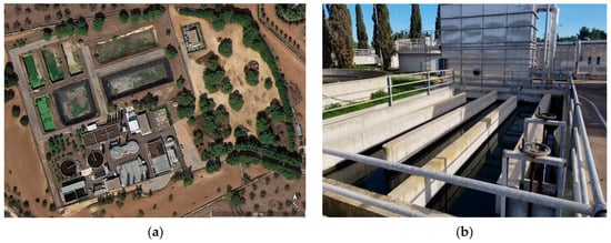
Figure 1.
(a) Detailed view of the plant layout highlighting the main treatment units; (b) photograph of the chlorine contact tank, which constitutes the subject of the hydraulics and CFD analyses presented in this study.
The chlorine contact tank is a rectangular reinforced concrete basin with internal vertical baffles creating a multi-chamber serpentine flow path. The tank has a nominal volume of ~80 m3, providing a hydraulic retention time of ~48 min at the design peak inflow of 0.0278 m3/s (100 m3/h). Wastewater enters via an inlet channel, flows sequentially through the baffle-separated chambers, and exits over an outlet weir (Figure 2).
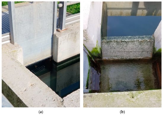
Figure 2.
Key structural components of the chlorine contact tank: (a) inlet channel directing wastewater into the first baffle-separated chamber; (b) outlet weir controlling effluent discharge at the end of the serpentine flow path.
In the baseline configuration (Figure 3), the tank features sharp 180° corners and straight-edged baffles with minimal fillets, which may induce recirculation behind the baffles and stagnant zones in interior corners, reducing hydraulic efficiency and deviating from ideal plug-flow behavior. Sodium hypochlorite (NaClO, 14–15% solution, ≥120 g/kg active chlorine) is continuously dosed at ~30 L/day (3.472 × 10⁻⁷ m3/s) in the inlet sump, primarily to protect downstream filtration. The flow path and baffle layout yield a length-to-width ratio > 40, favorable for mixing and achieving near plug-flow conditions. These hydraulic and dosing characteristics constitute the baseline for CFD analysis, enabling the assessment of residence time distributions, identification of dead zones and recirculation, and evaluation of potential geometric modifications to improve disinfection efficiency.
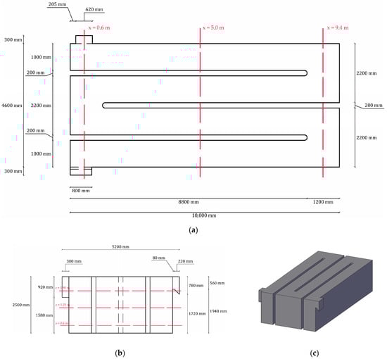
Figure 3.
Representation of the baseline configuration of the chlorine contact tank with section planes used for the analysis (red dotted lines): (a) top view, (b) frontal view, (c) three-dimensional perspective employed for CFD simulations.
2.1.2. Designed Alternative Configurations
To address the hydraulic limitations identified in the BC, two alternative design scenarios were developed and systematically evaluated.
ALT_1 (Rounded Corners, Figure 4a) entailed replacing all internal right-angle corners along the 180° channel turns with curved fillets of radius up to approximately 1.1 m. The objective of this intervention was to smooth the flow path by mitigating the sharp angles responsible for the generation of large low-velocity eddies. The inlet channel and outlet weir arrangements, as well as the positioning of the existing baffle walls, were preserved in this configuration to ensure comparability with the baseline case. ALT_2 (Perforated Baffles, Figure 4b) retained the rounded-corner geometry of ALT_1 while introducing additional modifications to the baffle walls. Specifically, three vertically aligned rectangular slots (0.10 m wide × 1.25 m high) were incorporated near the downstream end of each baffle, with a vertical spacing of 0.30 m center-to-center along the lower portion of the structure (Figure 4c). These openings were designed to allow a fraction of the flow to bypass the baffle edge, thereby attenuating recirculation behind the baffles and promoting a more uniform flow distribution across the channel cross-section.
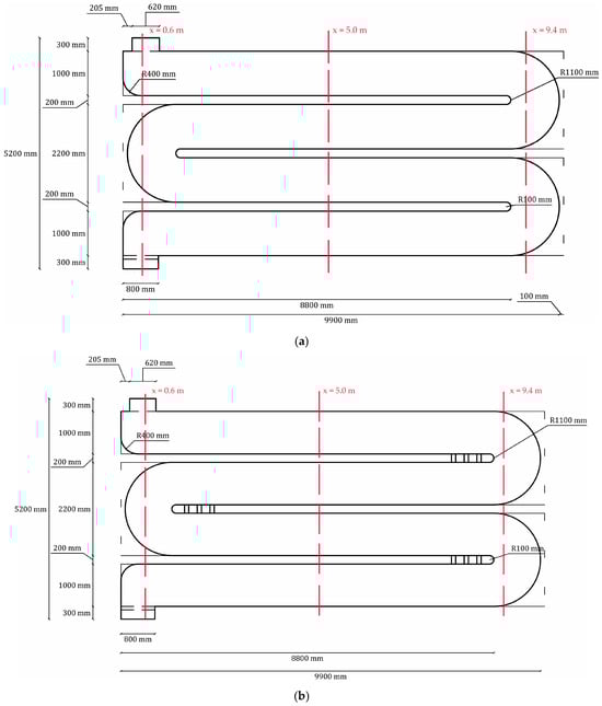
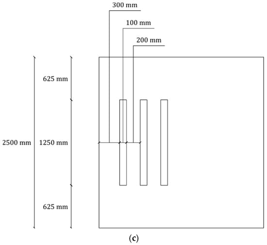
Figure 4.
Representation of the top view of the chlorine contact tank for the two alternative configurations with section planes used for the analysis (red dotted lines): (a) ALT_1—Rounded Corners, (b) ALT_2—Rounded Corners with Perforated Baffles, (c) ALT_2—Perforated Baffles dimensions.
Owing to slight differences in internal geometry, the total wet volume and associated nominal residence time (τ) varied among the configurations (Table 1): 80.45 m3 (τ ≈ 2894 s) for BC, 75.93 m3 (τ ≈ 2731 s) for ALT_1, and 77.06 m3 (τ ≈ 2772 s) for ALT_2, at a reference flow rate of Q = 0.0278 m3/s. For each configuration, independent CFD simulations were conducted to investigate (i) the hydrodynamic field (velocity distribution), (ii) conservative tracer transport for residence time distribution (RTD) analysis, and (iii) reactive transport including chlorine decay and pathogen inactivation.

Table 1.
Hydraulic parameters of the three tank configurations considered in the CFD simulations.
2.2. CFD Model Setup and Numerical Implementation
The hydrodynamics and tracer transport within the chlorine contact tank were simulated using the CFD solver FLOW-3D HYDRO (Flow Science, Inc., Santa Fe, NM, USA) [37], which resolves the three-dimensional Reynolds-Averaged Navier–Stokes (RANS) equations. Via a finite-volume approach, it is particularly suitable for free-surface flows through the Volume of Fluid (VOF) method [38]. These equations, written here in Cartesian coordinates, assuming the fluid is incompressible and viscous
being the fluid density, the water dynamic viscosity, the mean fluid pressure, (i = 1, 2, 3) the Cartesian coordinates that denote the mean components of the velocity , t and the time and the mean strain-rate tensor defined by
where the quantity is the Reynolds-stress tensor, a symmetric second-order tensor, where the diagonal components are normal stresses, whereas the off-diagonal elements are shear stresses. This formulation introduces six unknown components of the symmetric tensor without additional equations, so the defined system is undetermined. Turbulent flow, which ensures the system is closed, was modeled using the Renormalized Group (RNG) k − ε model [39,40,41], a variant of the standard k − ε model [42] that provides improved accuracy for flows with high strain and swirl features [43], with the turbulent mixing length dynamically computed by the solver. The distribution of k and ε are calculated from the following semi-empirical modeled transport equations:
where k represents turbulent kinetic energy, VF, Ax, Ay, Az represents the FAVORTM [37] functions, P represents the production of turbulent kinetic energy, G represents the buoyancy production, Diff represents the diffusivity, ε represents the dissipation rate, CDIS1, CDIS2, CDIS3 are all dimensionless user-adjustable parameters, with predefined values of 1.44, 192, and 0.2, respectively.
In FLOW-3D HYDRO the RNG k − ε model still provides the core turbulence fields and and computes an eddy viscosity used in the Boussinesq closure for the Reynolds stresses [37]. The wall function acts as the near-wall boundary condition: using the log-law it converts the local near-wall mean velocity and the wall-distance into a friction velocity hence a wall shear and prescribes consistent near-wall values of and . Those values feed back into turbulent eddy viscosity and therefore into the Reynolds-stress term in the momentum equations, closing the loop [37].
The tracer convection-diffusion equation has the following form:
In which CSOR is a source term.
In FLOW-3D HYDRO the concentration equation is closed through the gradient diffusion hypothesis, so the unresolved correlation is not written explicitly. Instead, it is modeled as a diffusive flux using the turbulent diffusivity , where comes from the RNG model and is the turbulent Schmidt number. Therefore, although the authors did not specify the functions and coefficients in their written equation, FLOW-3D provides them internally through its turbulence model and scalar-diffusion closure. The RNG eddy viscosity determines the turbulent transport, making an explicit double correlation term unnecessary [37]. It is important to highlight that, for chlorine transport, the velocity–concentration correlation is modeled using a constant Schmidt number and turbulent viscosity, without an explicit near-wall closure, relying instead on a predictor–corrector scheme for numerical convergence.
This solver is specifically designed to use the VOF method, which employs a phase-fraction-based approach to capture the position and evolution of the free surface elevation (FSE). The VOF technique [44,45] represents each fluid phase: in this case, water and air, by a volume fraction within each computational cell. A cell entirely filled with air is assigned a volume fraction of 0, whereas a cell completely occupied by water has a value of 1; intermediate values indicate the presence of the interface between the two phases. The indicator function, ζ, describing the fluid distribution in the domain, is expressed as
By treating the two-phase system as a homogenized mixture, the effective properties of the fluid, namely density and dynamic viscosity, are obtained as weighted averages of the individual phases, defined as
respectively, where subscripts 1 and 2 refer to the specific phases considered. This formulation allows the solver to capture complex interface dynamics while maintaining numerical stability and computational efficiency. This technique allows us to locate and track the free surface, providing satisfactory results [46,47,48].
The tank geometry was generated in CAD and imported as an STL file into the CFD environment. As far as the discretization of the computational domain is concerned, a structured mesh was built. Various numerical tests were performed before reaching the final configuration of the grid, employing an increasing number of cells in all directions and controlling the consistency of the RTD indices within acceptable limits.
The final three-dimensional finite-volume computational domain (Figure 5) includes about 291,000 grid points.
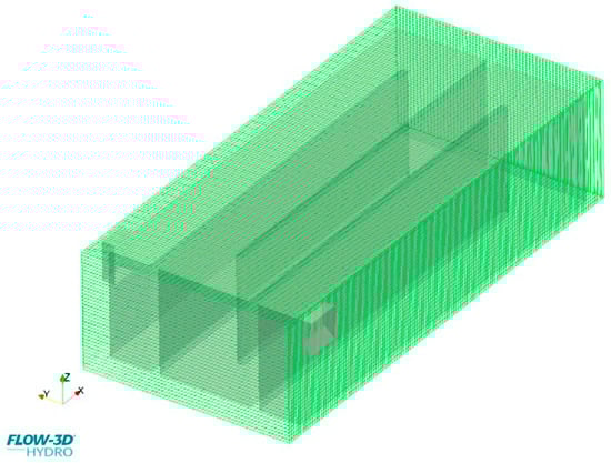
Figure 5.
Computational mesh adopted for the CFD simulations of the chlorine contact tank, generated with a uniform grid size of 0.08 m (≈291,000 cells). Local refinement is shown near the walls and baffle slots to improve the resolution of flow features.
Boundary conditions were defined as a specified volumetric flow rate at the inlet (0.0278 m3/s) with a fluid elevation of 2.01 m, and a pressure outlet at the weir crest with a fixed elevation of 1.94 m, resulting in flow driven by a slight head difference and maintaining an average water depth of approximately 1.9–2.0 m. The free surface was captured with the VOF method under an open-top atmospheric condition. At the walls, the standard wall function approach was applied. At these points the velocity distribution was assumed to follow the logarithmic law of the wall which forms the boundary condition for the velocity parallel to the wall. At rigid walls (tank bottom, sides, and baffle surfaces), the values of k, ε and C were set equal to zero.
Simulations were initialized with a hydrostatic water column at rest up to the outlet weir elevation, and the flow field was first resolved for a sufficient duration (~2000 s of simulated time) to reach quasi steady-state conditions, monitored through a control section and a small control volume positioned at the outlet weir. The resulting flow field was then used as the starting condition for tracer and reactive transport simulations. In these simulations, the conservative tracer was initialized at zero in the flow field simulation and released at a concentration of 1 kg/m3 for a duration corresponding to 5% of the nominal residence time, with a turbulent diffusion coefficient scaled by a Schmidt number of 1.43. This modeling framework enabled the assessment of internal flow patterns, identification of recirculation and stagnant zones, and evaluation of chlorine transport and decay under realistic operational conditions.
2.3. Residence Time Distribution Theory and Hydraulic Efficiency Indices
To assess the hydraulic performance of the tank, tracer simulations were conducted to generate residence time distribution (RTD) curves for each configuration [49]. In these simulations, a small quantity of a conservative tracer was injected at the inlet as an impulse, representing a brief pulse input [50]. Following the established guidelines, the duration of the injection was set to 5% of the nominal residence time, τ [51]. For instance, in the baseline configuration (BC), τ ≈ 2894 s, resulting in a tracer injection period of approximately 145 s. During this interval, the tracer concentration at the inlet was maintained at a fixed reference value of 1.0 kg/m3 and subsequently reset to zero after the pulse. This procedure approximates a Dirac delta input relative to the system time scale, ensuring a sharp RTD signal. Previous studies indicate that maintaining the injection duration below 5% of τ minimizes distortion of the RTD curve [52,53,54].
The tracer was modelled as a passive, non-reactive scalar, transported according to the scalar transport equation implemented in FLOW-3D. Turbulent diffusion was accounted for by applying a turbulent diffusion coefficient 1.43 times than the turbulent viscosity, implemented in the solver through a “turbulent diffusion multiplier”. As the tracer propagated through the tank and exited over the outlet weir, the effluent concentration was monitored over time using a dedicated control surface at the weir. From the resulting time series, the RTD function E(θ) was computed, where θ = t/τ represents the dimensionless time. The concentration measurements were converted to the residence time distribution function using the standard formula:
Here, C(t) denotes the tracer concentration in the effluent at time t, Cinit represents the injected tracer concentration (1 kg/m3), and Tinjection is the duration of the tracer injection. This normalization guarantees that the area under the RTD curve E(θ) is equal to 1. The cumulative residence time distribution, F(θ), can be obtained by integrating E(θ) from 0 to θ, representing the fraction of fluid that has exited the reactor at a given dimensionless time.
Once the RTD curves were obtained, key hydraulic efficiency indices were derived to evaluate the performance of the contact tank. The baffling factor, θ10 [55], corresponds to the dimensionless time at which 10% of the tracer has exited (i.e., F(θ10) = 0.1). In dimensional terms, t10 = θ10, indicates the time by which the earliest 10% of fluid has left the tank. Higher values of θ10, approaching 1, indicate reduced short-circuiting and more ideal plug-flow behavior [56], whereas lower values reflect increased mixing or dead zones. In practical applications, θ10 values greater than 0.7 are generally considered acceptable for efficient hydraulic performance. The Morrill index (Mo) was calculated as:
where is the dimensionless time required to observe 90% of the tracer concentration at the outlet of the contact tank. This index quantifies the time span between the exit of 10% and 90% of the tracer relative to the median residence time and provides a measure of mixing and dispersion within the tank. For an ideal plug-flow reactor, Mo equals 1, as θ10 = θ90. Deviations from this value indicate a broader distribution of residence times. Lower Mo values correspond to more uniform residence times, with values below 2 considered indicative of very good hydraulic performance, whereas higher values (Mo > 5) suggest excessive mixing and the presence of dead zones [12].
The Aral–Demirel index (AD) [12] was calculated as:
which combines information on both short-circuiting and tailing within the tank. The AD index is used to evaluate both hydraulic behavior and mixing performance in a contact tank.
Low AD values indicate poor mixing and strong short-circuiting, while high AD values indicate good mixing and minimal short-circuiting. For clearer performance categories: AD < 0.2 denotes poor performance, 0.2 < AD < 0.5 as fair, 0.5 < AD < 1.75 as compromising, 1.75 < AD < 3.5 as good, and AD > 3.5 as excellent.
New geometrical parameter proposed by [32], based on region occupied by the stable reversal flows, is investigated. This parameter is defined as Recirculation Factor (RF) and is calculated according to the following equation:
where Vr is the volume of tank occupied by the recirculation zones and Vtot is the overall volume of the reactor. The RF coefficient spans the range [0–1]. It assumes an ideal value of 0 when the entire tank volume is occupied by eddies and dead zones. On the other hand, it is equal to 1 in ideal plug flow conditions, where no recirculation regions occur.
These indices provide a semi-quantitative measure of hydraulic performance. While they do not capture all details of the flow field, as they reduce the RTD curve to a few representative numbers, they are useful for comparing different tank configurations. In the present study, θ10, θ90, Mo, AD, and RF were calculated for each scenario by processing the CFD-simulated RTD curves. Data analysis was performed using a MATLAB R2024a routine that read the effluent concentration time series and computed the cumulative distribution along with the required percentiles.
2.4. Reaction Kinetics Simulation
In addition to the passive tracer simulations, reactive species transport simulations were conducted to model both chlorine decay and microbial inactivation within the contact tank. Modeling these reactions is essential because microbial inactivation is not the only relevant chemical process in the tank: chlorine decay directly affects disinfection rates, and regulatory requirements mandate specific residual chlorine concentrations in treated effluent. Furthermore, the formation of potentially hazardous chlorinated by-products highlights the importance of simulating chlorine kinetics to support both the design and evaluation of existing contact tanks. Accurate representation of these reactions is challenging, as they depend on several factors, including water composition, temperature, initial chlorine concentration, pH, and the maintenance of chlorine levels over time [57,58].
Chlorine is typically dosed as a gas or as a sodium or calcium hypochlorite solution. Besides acting as a biocide, chlorine reacts with organic and inorganic matter, resulting in decay [56]. The reaction of chlorine gas with water can be expressed as:
Similar reactions occur with hypochlorite solutions. A standard first-order decay model can be written as [57]:
where t is time in hours, C0 is the initial chlorine concentration (mg/L), and kb is the first-order decay constant, which typically ranges between 0.02 and 0.74 h−1 and depends on temperature, organic content, and initial chlorine dose [59,60,61,62]. In the present investigation, a decay constant was chosen and tuned such that the predicted residual chlorine at the outlet matched field measurements. Observed residuals at the outlet were approximately 0.05–0.1 mg/L, consistent with literature values. The chlorine decay was implemented in FLOW-3D via its species reaction module (i.e., the “Reaction Kinetics” option), applying a global first-order decay to the chlorine concentration field throughout the tank. Microbial inactivation was modeled using a Chick-Watson type kinetic expression [63]:
where N is the concentration of viable microorganisms, denotes the local chlorine concentration, n is the disinfectant demand exponent (approximately 1 for chlorine), and k′ is an empirical disinfection rate coefficient. The value of k′ is system-specific, influenced by microorganism type, water chemistry, disinfectant properties, temperature, and pH, and must be calibrated to reflect practical conditions. In the present simulations, k′ was set to produce measurable log reductions across the tank, with the primary goal of assessing relative differences in disinfection performance under the given hydraulic conditions rather than absolute microbial removal. The reactive simulation was conducted until the flow reached quasi-steady-state conditions, with a constant chlorine dose applied at the inlet while simultaneously tracking the concentration fields of both chlorine and microorganisms throughout the tank.
Moreover, for validation purposes, a limited number of grab samples of residual chlorine were collected at the actual outlet weir of the BC plant using a portable chlororesiduometer.
3. Results
This section presents and discusses the results obtained from the conducted simulations and analyses. Specifically, Section 3.1 reports the outcomes related to model validation; Section 3.2 presents the flow field results and provides a qualitative analysis of the hydraulic behavior; Section 3.3 details the RTD results along with the computed hydraulic efficiency indices; finally, Section 3.4 focuses on the disinfection kinetics and chlorine distribution within the contact tank.
3.1. Model Validation
Due to operational and safety constraints, it was not possible to conduct a full-scale experimental campaign on the contact tank under operating conditions. Nevertheless, grab samples of residual chlorine were collected near the outlet weir using a portable chlororesiduometer to support model validation. Samples were taken at a depth of ~1 m depth from the free surface, with a sampling interval of about six minutes, corresponding to the time required for collection and preparation. In the computational domain, a virtual probe was positioned at the same location as the field sampling point, ensuring consistency in the comparison between measured and simulated data. Field measurements indicated residual chlorine concentrations on the order of 0.05 mg/L (from an initial dose of approximately 1–2 mg/L). After calibration of the decay coefficient, CFD simulations reproduced these values with acceptable agreement, having deviations below 0.01 mg/L. Figure 6 presents the comparison between the simulated chlorine concentrations and the average of field measurements, demonstrating that the model adequately captured the reaction kinetics.
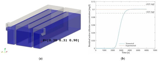
Figure 6.
(a) Location of the sampling/monitoring point adopted for both field measurements and numerical simulations; (b) comparison between measured and simulated residual active chlorine concentrations at the outlet.
3.2. Flow Field and Qualitative Hydraulic Behavior
The CFD simulations highlighted several non-ideal hydrodynamic features in BC, confirming the initial concerns regarding tank performance. Section planes used for the analysis are reported in Figure 3 and Figure 4a,b. The analysed x-planes are located at z = 0.6 m, 1.25 m, and 1.9 m, while the analysed z-planes are located at x = 0.6 m, 5.0 m, and 9.4 m.
Representative velocity vector plots for the BC case are shown in Figure 7. In the first 180° bend, the incoming jet impinges on the end wall and reverses direction, forming a large recirculation zone immediately behind the baffle (Figure 8a–c). A similar vortical separation is observed at the outlet bend, downstream of the last baffle. In both cases, the reversed velocity vectors clearly indicate localized flow separation. In addition, stagnant pockets characterized by near-zero velocities develop in the inner corners of the bends (Figure 8a–c), where water is effectively bypassed by the main stream. Velocity contours confirm the presence of these poorly exchanged regions, with magnitudes approaching zero.
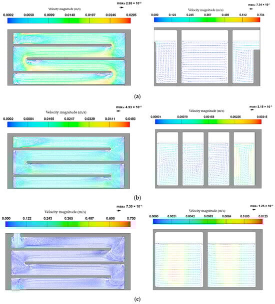
Figure 7.
Z-planes and x-planes views of representative velocity vector for BC: (a) z = 0.6 m and x = 0.6 m, (b) z = 1.25 m and x = 5.0 m, (c) z = 1.9 m and x = 9.4 m.
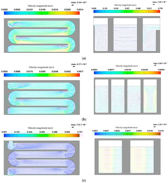
Figure 8.
Z-planes and x-planes views of representative velocity vector for ALT_1: (a) z = 0.6 m and x = 0.6 m, (b) z = 1.25 m and x = 5.0 m, (c) z = 1.9 m and x = 9.4 m.
The implications of these flow structures are twofold. First, recirculation and stagnation zones extend the residence time of water trapped within them, potentially leading to excessive chlorine exposure and increased risk of disinfection by-product formation. Second, the effective volume available for plug flow is reduced, since part of the tank is excluded from the main flow-through. Flow tends to shortcut along the outer walls of the bends, with velocities around 0.2–0.3 m/s, compared to an expected mean velocity of approximately 0.1 m/s for ideal plug flow. As a result, a fraction of the influent exits significantly earlier than the nominal contact time of 48 min. Tracer simulations indicated that about 10% of the influent water exited in only 0.87 of the nominal retention time (θ10 ≈ 0.87), confirming the presence of short-circuiting. Overall, the flow field in BC represents a combination of plug flow behavior in some regions and complete mixing in others, a typical condition for imperfectly baffled contact tanks.
The modifications introduced in ALT_1 led to a substantial reduction in the stagnation pockets located in the inner corners of the bends (Figure 8a–c).
Replacing sharp 90° corners with quarter-circle fillets allowed the flow to remain attached to the curved wall and prevented the formation of large recirculation zones in those areas. As a consequence, the previously stagnant volumes were effectively re-engaged in the flow, leading to an increase in the usable hydraulic volume. However, flow separation downstream of the baffle tips persisted with similar intensity as in BC, since the sharp geometry of the baffles was not altered. Although secondary vortices appeared weaker at intermediate cross-sections, eddies in the wake of the baffles remained a limiting feature.
ALT_2 provided the most favorable flow conditions among the tested configurations (Figure 9a–c).
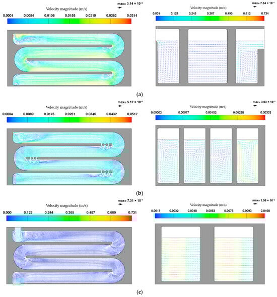
Figure 9.
Z-planes and x-planes views of representative velocity vector for ALT_2: (a) z = 0.6 m and x = 0.6 m, (b) z = 1.25 m and x = 5.0 m, (c) z = 1.9 m and x = 9.4 m.
The introduction of perforated baffles, combined with rounded corners, significantly reduced both stagnation and recirculation zones. The flow through the baffles was obtained by defining measurement sections in the perforations and integrating the velocity over these areas using the software’s post-processor. Approximately 10–20% of the flow passed through the baffle orifices, effectively flushing areas that were previously disconnected from the main stream. The eddies behind the baffles were either strongly reduced or entirely suppressed, and the redistribution of momentum across the channels mitigated the high-velocity streaks along the outer walls. Consequently, ALT_2 promoted a more balanced velocity field, with a more uniform outlet profile and reduced short-circuiting compared to BC and ALT_1. Overall, ALT_2 provided hydraulic conditions closer to the ideal plug flow regime, with a larger fraction of the total volume effectively contributing to the contact process.
The qualitative observations described above highlight how BC suffers from both corner stagnation and baffle-induced recirculation (Figure 7a,b). ALT_1 partially addresses the first issue but leaves the second largely unresolved (Figure 8a,b), while ALT_2 combines both design modifications to approach near plug flow conditions (Figure 9a,b). The main hydraulic features of the three configurations are summarized in Table 2.
Table 2.
Summary of flow characteristics for the three configurations (BC, ALT_1, ALT_2).
3.3. Residence Time Distributions and Hydraulic Indices Results
The RTD curves for the three configurations are shown in Figure 10. In BC, E(θ) exhibits a broad distribution with an early rise at θ ≈ 0.3–0.4, a peak at θ ≈ 0.8, and a long tail beyond θ = 1.5. This pattern reflects marked deviations from ideal plug flow, with both short-circuiting (early breakthrough) and stagnation (extended tailing).
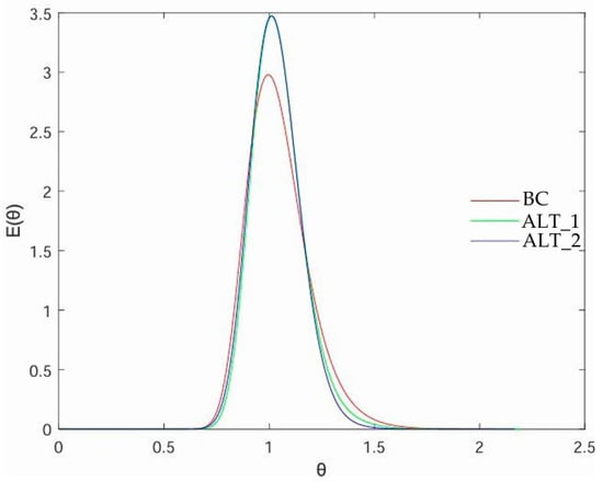
Figure 10.
Residence time distribution (RTD) curves for the analyzed configurations: BC, ALT_1, ALT_2.
In contrast, ALT_1 and ALT_2 display much narrower distributions, concentrated around θ = 1. Their curves are nearly superimposed, both characterized by a sharper peak and a more symmetric profile relative to BC. This indicates that the main improvement was already achieved by ALT_1 through the elimination of stagnant corners, while the additional perforation s introduced in ALT_2 had only a marginal effect on the overall cumulative RTD. Nonetheless, both alternatives outperform BC: their peaks are higher, while the tails are shorter, and premature breakthrough is almost entirely suppressed.
The quantitative analysis of F(θ) (Figure 11) and the derived indices (Table 3) confirm these trends. For θ10, BC yielded 0.8747, while ALT_1 and ALT_2 increased this value to 0.8965 and 0.8871, respectively. The higher values indicate delayed initial breakthrough, with ALT_1 achieving the greatest improvement (+2.5% relative to BC). For θ90, ALT_2 obtained the lowest value (1.1838), representing a 4.1% reduction compared with BC (1.2348), while ALT_1 also improved performance (1.2018, −2.7% vs. BC). These reductions in θ90 demonstrate that both alternatives effectively limit tailing, with ALT_2 performing best.
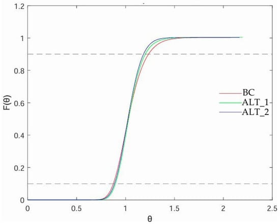
Figure 11.
Cumulative residence time distributions F(θ) for the analyzed configurations: BC, ALT_1, ALT_2.
Table 3.
Hydraulic efficiency indices for the analyzed configurations: BC, ALT_1, ALT_2.
Mo index decreased from 1.4116 in BC to 1.3405 in ALT_1 and 1.3345 in ALT_2, indicating narrower RTDs in both alternatives. ALT_2 achieved the lowest value, about 5.5% lower than BC. Similarly, the AD index decreased from 1.8741 (BC) to 1.6274 in ALT_2. ALT_1, instead, reached 1.9497, slightly higher than BC. This small difference remains within the expected range for baffled contactors (0.1–2.5). The alternative ALT_2 was proposed to have less short-circuiting and good mixing. Although Figure 9 shows a reduction in both stagnation and recirculation zones, we believe that the lower value of AD is due to the not optimized position of the perforated baffles.
RF index increased from 0.478 in ALT_2 to 0.512 in ALT_1 and 0. 478 in BC. ALT_2 achieved the lowest value, about 16.9% lower than BC.
In summary, both alternatives improved the hydraulic efficiency of the system by narrowing the RTD and reducing deviations from τ. ALT_1 was the most effective in delaying the early breakthrough, while ALT_2 achieved the best overall performance, with the lowest θ90, the minimum Mo, and the AD value comparable to the other cases. Although the percentage differences are modest, even small increases in θ10 or reductions in Mo are operationally relevant, as they directly contribute to more reliable disinfection performance.
3.4. Disinfection Kinetics and Chlorine Distribution Results
The implications of the hydraulic scenarios on disinfection performance can be inferred qualitatively from the flow patterns and RTD results.
In BC, short-circuiting causes a fraction of the flow to receive substantially less contact time with chlorine than intended, which would likely reduce microbial inactivation and allow pathogens to persist at the outlet. Conversely, water trapped in recirculation zones experiences extended residence times; however, since little fresh chlorine is transported into these eddies, the initial chlorine dose is rapidly consumed, creating regions with poor disinfection efficiency. Prolonged retention in stagnant zones also increases the risk of forming chlorinated by-products. The CFD results for BC confirmed this heterogeneity: along the main flow path, chlorine decayed rapidly due to continuous reaction and insufficient contact time, while recirculation zones initially preserved chlorine longer but eventually became depleted pockets once the initial residual was exhausted. The net effect is inefficient; a part of the chlorine is wasted in zones with no benefit after pathogens are already inactivated, while another part of the flow remains under-treated.
These limitations are mitigated in the improved configurations. In ALT_1, the elimination of stagnant corners ensures that nearly all water parcels pass through active flow regions, reducing “wasted volume” and improving exposure to disinfectant. In ALT_2, the introduction of baffle orifices further enhances performance by promoting mixing between the main stream and recirculation zones, ensuring a more uniform chlorine distribution. Consequently, for a given chlorine dose, ALT_2 is expected to achieve slightly higher pathogen inactivation than BC or ALT_1, as fewer particles escape with short contact and a greater fraction of the volume experiences adequate disinfection. Since pathogen inactivation depends largely on the Ct, the product of chlorine concentration and contact time, even a 2–5% increase in the minimum exposure can significantly improve efficacy for the fraction of flow that was previously under-treated.
The calibrated kinetic simulation for BC predicted approximately 1 log (90%) inactivation of the target organism under typical operating conditions (e.g., 45–50 min of contact time at ~0.5 mg/L residual chlorine). In ALT_2, this reduction could plausibly increase to 1.1–1.2 log, or alternatively, the same 1-log target could be achieved with a lower applied chlorine dose, thereby reducing chemical demand. Moreover, by attenuating RTD tailing, ALT_2 also limits over-exposure of certain flow parcels, potentially decreasing the formation of disinfection by-products such as trihalomethanes (THMs). This dual effect, enhanced microbial inactivation with reduced by-product formation, represents a relevant operational advantage of the modified design.
4. Discussion
The CFD analysis of the contact tank demonstrates that relatively small geometric modifications can lead to substantial improvements in hydraulic performance. Although BC includes baffle walls to extend the flow path, short-circuiting and dead zones persist. These inefficiencies, widely reported in the literature, were confirmed here: flow separation at sharp corners and baffle edges created recirculation zones that diverted a part of the flow and reduced the effective contact volume. Consequently, the RTD deviates from ideal plug flow, with some water exiting prematurely and other fractions retained excessively. From a design perspective, BC may be classified as “good but not excellent”: θ10 ≈ 0.87 and Mo ≈ 1.41 indicate moderate baffling but still a significant deviation from plug flow (θ10 → 1, Mo → 1). While the tank meets disinfection requirements under conservative conditions, improving hydraulic performance provides an additional safety margin and operational benefits, including potentially lower chlorine doses for the same pathogen inactivation.
The two modifications tested in this study leverage established strategies for plug-flow enhancement:
ALT_1 (corner rounding): sharp corners promote eddy formation. By rounding these corners, recirculation zones along inner walls were eliminated, allowing flow to sweep the corners more effectively and recover previously inactive volume. This outcome aligns with practical experience, where chamfered corners or guide plates are commonly used in new or retrofitted tanks to reduce dead zones.
ALT_2 (baffle perforations): complete channel segregation by baffles can produce stagnant eddies at channel ends. Introducing orifices allowed controlled cross-communication between compartments, effectively flushing recirculation zones behind baffle tips. This approach permits a small, controlled short-circuit to eliminate uncontrolled stagnation. ALT_2 achieved the lowest dead-zone fraction and the most favorable hydraulic indices. The specific configuration used (three 10 × 125 cm slots per baffle) represents one feasible design, and further optimization of size or placement could enhance performance. Interestingly, RTD curves for ALT_1 and ALT_2 were nearly identical, indicating that corner rounding drives the bulk improvement in RTD, while perforations reduce localized recirculation and homogenize the velocity field, enhancing robustness under variable flow conditions.
The hydraulic improvements have clear implications for disinfection. In ALT_2, the entire tank volume is more effectively utilized, ensuring that the design contact time (~48 min) is more uniformly achieved. This increases confidence in meeting regulatory targets (e.g., pathogen log reduction, minimum residual chlorine) and may allow slightly lower chlorine doses, reducing chemical demand. Moreover, minimizing stagnant volume lowers the risk of forming chlorinated by-products, an important consideration for effluent reuse. Although field verification (e.g., tracer or disinfection tests) is necessary, the CFD results provide strong evidence supporting these trends.
Practical implementation of these modifications requires consideration. Corner rounding (ALT_1) could be achieved using inserts or concrete bevelling, while baffle perforations (ALT_2) involve cutting slots, reinforcing the structure, and ensuring resistance to debris accumulation. While these interventions entail costs, CFD indicates they are worthwhile, particularly ALT_2, which yielded the best hydraulic performance and eliminated residual recirculation. If only one modification is feasible, prioritizing baffle perforations (ideally combined with corner rounding) is recommended. Additional refinements, such as adjusting orifice geometry or tapering baffle edges, could further optimize flow.
Finally, this study highlights the diagnostic and predictive value of CFD. Traditional tracer studies provide bulk RTD information but limited insight into internal flow dynamics. CFD complements such approaches by visualizing flow fields, identifying recirculation zones, and enabling low-cost evaluation of multiple design scenarios. This capability allows iterative design optimization prior to expensive physical modifications, supporting more efficient and robust tank operation.
5. Conclusions
This study presented a CFD-based analysis of the chlorine contact tank of a wastewater treatment plant, focusing on hydraulic performance and potential design improvements. FLOW-3D HYDRO simulations of flow, tracer dispersion, and chlorine decay provided detailed insights into tank hydrodynamics that are otherwise difficult to obtain.
The existing configuration exhibited significant hydraulic inefficiencies, including recirculation zones behind baffles and stagnant water in sharp corners. These features caused deviations from plug flow, as reflected in a broad RTD and hydraulic indices (θ10 ≈ 0.87, Mo ≈ 1.41), resulting in premature exit of some water fractions and over-retention of others. Such conditions may reduce disinfection efficiency and increase the risk of by-product formation.
The key findings of the study are as follows:
- Design improvements: ALT_1, with rounded corners, eliminated dead zones at channel turns and improved effective volume utilization. ALT_2, which combined rounded corners with perforated baffles, further disrupted recirculation behind baffles, achieving the most plug-flow-like behaviour and the best hydraulic indices. While ALT_1 increased θ10 by approximately 2.5%, ALT_2 additionally homogenized flow and minimized recirculation, enhancing overall tank efficiency;
- Disinfection implications: improved hydraulics in ALT_2 ensure more uniform contact times (~48 min), allowing consistent pathogen log reduction with potentially lower chlorine doses. Minimization of stagnant zones also reduces overexposure and the formation of chlorinated by-products, improving treatment safety and effluent quality;
- Practical recommendations: implementing ALT_2 is recommended to maximize hydraulic and disinfection performance. Corner rounding can be achieved with inserts or concrete beveling, while baffle perforations require slotting with structural reinforcement. Further optimization of orifice geometry, placement, or baffle shaping could provide additional benefits.
Field validation (e.g., tracer tests or microbial assays) is necessary to confirm predicted improvements based on CFD simulations. Although the present study demonstrates that CFD can effectively capture the overall hydrodynamics and scalar transport characteristics of a chlorine contact tank, providing useful insights into flow distribution, mixing behavior, and disinfectant concentration fields, the modeling framework employed here relies on the standard gradient-diffusion hypothesis with a constant turbulent Schmidt number, together with turbulence viscosity–based scalar transport. These assumptions inherently simplify the dual velocity–concentration correlation and do not include an explicit near-wall closure for chlorine transport. As a result, the predicted concentration fields may be sujected to uncertainty, particularly in regions with strong turbulence anisotropy or significant near-wall scalar gradients. Therefore, the results presented should be interpreted with these limitations in mind, and further verification using more advanced turbulent transport models.
Future work could explore optimization of baffle geometry, size, and placement, or alternative flow-guiding strategies such as angled or tapered baffles. The methodology is broadly applicable to other contact tanks or hydraulic reactors, supporting design improvements and retrofits in various contexts. Overall, relatively simple geometric modifications, particularly the ALT_2 design, significantly improve hydraulic performance and approach plug-flow behaviour, enhancing disinfection reliability, chemical efficiency, and operational safety. CFD proved valuable for diagnosing inefficiencies and evaluating design alternatives prior to physical modification, offering actionable guidance for targeted engineering interventions and more efficient wastewater treatment design.
Author Contributions
Conceptualization, G.R.T., A.T., A.L. and P.L.; methodology, A.T., A.L. and P.L.; software, A.T., A.F.M., N.F. and F.L.; validation, A.T., E.L., A.F., N.F. and F.L.; formal analysis, A.T., E.L., A.F., N.F. and F.L.; investigation, E.L., A.F., N.F., F.L. and A.L.; resources, A.F.M.; data curation, A.F.M., N.F. and F.L.; writing—original draft preparation, A.T., E.L., A.F., A.L. and P.L.; writing—review and editing, A.T., E.L., A.F., A.L. and P.L.; visualization, G.R.T., E.L., A.F., N.F., F.L. and P.L.; supervision, G.R.T., A.L. and P.L.; project administration, A.L., F.D. and P.L. All authors have read and agreed to the published version of the manuscript.
Funding
This research received no external funding.
Institutional Review Board Statement
Not applicable.
Informed Consent Statement
Not applicable.
Data Availability Statement
The data presented in this study are available on request from the corresponding author.
Acknowledgments
The authors would like to thank Acquedotto Pugliese SpA, particularly Fabrizio Dell’Anna and Desio Carparelli, for their kind cooperation and for granting access to one of their facilities. This access significantly contributed to the scientific and technical insights developed in this work.
Conflicts of Interest
The authors declare no conflicts of interest.
Abbreviations
The following abbreviations are used in this manuscript:
| CFD | Computational Fluid Dynamics |
| WWTP | Wastewater Treatment Plant |
| BC | Baseline Configuration |
| ALT_1 | Alternative Configuration 1 |
| ALT_2 | Alternative Configuration 2 |
| RTD | Residence Time Distribution |
| Mo | Morrill index |
| AD RF | Aral–Demirel index Recirculation Factor |
| FSE | Free Surface Elevation |
| VOF | Volume of Fluid |
| RANS | Reynolds-Averaged Navier–Stokes Equation |
| RNG | Renormalized Group |
| THMs | Trihalomethanes |
References
- Angeloudis, A.; Stoesser, T.; Falconer, R.A. Predicting the disinfection efficiency range in chlorine contact tanks through a CFD-based approach. Water Res. 2014, 60, 118–129. [Google Scholar] [CrossRef]
- Mazhar, M.A.; Khan, N.A.; Ahmed, S.; Khan, A.H.; Hussain, A.; Changani, F.; Yousefi, M.; Ahmadi, S.; Vambol, V. Chlorination disinfection by-products in municipal drinking water–a review. J. Clean. Prod. 2020, 273, 123159. [Google Scholar] [CrossRef]
- Hrudey, S.E. Chlorination disinfection by-products, public health risk tradeoffs and me. Water Res. 2009, 43, 2057–2092. [Google Scholar] [CrossRef] [PubMed]
- Bull, R.J.; Birnbaum, L.; Cantor, K.P.; Rose, J.B.; Butterworth, B.E.; Pegram, R.E.X.; Tuomisto, J. Water chlorination: Essential process or cancer hazard? Toxicol. Sci. 1995, 28, 155–166. [Google Scholar] [CrossRef]
- Du, Y.; Lv, X.T.; Wu, Q.Y.; Zhang, D.Y.; Zhou, Y.T.; Peng, L.; Hu, H.Y. Formation and control of disinfection byproducts and toxicity during reclaimed water chlorination: A review. J. Environ. Sci. 2017, 58, 51–63. [Google Scholar] [CrossRef]
- Younis, A.; Ebead, U.; Suraneni, P.; Nanni, A. Cost effectiveness of reinforcement alternatives for a concrete water chlorination tank. J. Build. Eng. 2020, 27, 100992. [Google Scholar] [CrossRef]
- Wilson, J.M.; Venayagamoorthy, S.K. Evaluation of hydraulic efficiency of disinfection systems based on residence time distribution curves. Environ. Sci. Technol. 2010, 44, 9377–9382. [Google Scholar] [CrossRef]
- Maslak, D.; Weuster-Botz, D. Combination of hydrodynamic cavitation and chlorine dioxide for disinfection of water. Eng. Life Sci. 2011, 11, 350–358. [Google Scholar] [CrossRef]
- Shoshaa, R.; Ghanimeh, S.; Almomani, F. Recent advances in plug flow reactors for anaerobic digestion and in-depth evaluation of mixing approaches: A review. Fuel 2024, 377, 132711. [Google Scholar] [CrossRef]
- Li, Y.; Skyllas-Kazacos, M.; Bao, J. A dynamic plug flow reactor model for a vanadium redox flow battery cell. J. Power Sources 2016, 311, 57–67. [Google Scholar] [CrossRef]
- Gualtieri, C.; Doria, G.P. Residence time distribution and dispersion in a contact tank. In Proceedings of the Congress-International Association for Hydraulic Research, Venice, Italy, 1–6 July 2007; Volume 32, p. 486. [Google Scholar]
- Demirel, E.; Aral, M.M. Performance of efficiency indexes for contact tanks. J. Environ. Eng. 2018, 144, 04018076. [Google Scholar] [CrossRef]
- Mofidi, A.A.; Linden, K.G.; Bedell, E.; Vetrovs, A.; Friedman, M.; Won, D.; Deem, S.; Rice, N.; Jahne, M.; Nicholas, T.; et al. Development of a disinfection efficiency database for bacterial inactivation: A systematic literature review for selected water treatment technologies. Crit. Rev. Environ. Sci. Technol. 2025, 55, 1413–1429. [Google Scholar] [CrossRef]
- Wang, D.; Chen, X.; Luo, J.; Shi, P.; Zhou, Q.; Li, A.; Pan, Y. Comparison of chlorine and chlorine dioxide disinfection in drinking water: Evaluation of disinfection byproduct formation under equal disinfection efficiency. Water Res. 2024, 260, 121932. [Google Scholar] [CrossRef] [PubMed]
- Hua, P.; Wang, Z.; Wang, H.; de Oliveira, K.R.F.; Ying, G.G. CFD simulation of spatiotemporal distribution of residual chlorine in secondary water supply tanks. Environ. Sci. Water Res. Technol. 2023, 9, 2903–2915. [Google Scholar] [CrossRef]
- Kizilaslan, M.A.; Nasyrlayev, N.; Kurumus, A.T.; Savas, H.; Demirel, E.; Aral, M.M. Experimental and numerical evaluation of a porous baffle design for contact tanks. J. Environ. Eng. 2020, 146, 04020063. [Google Scholar] [CrossRef]
- Cheswick, R.; Nocker, A.; Moore, G.; Jefferson, B.; Jarvis, P. Exploring the use of flow cytometry for understanding the efficacy of disinfection in chlorine contact tanks. Water Res. 2022, 217, 118420. [Google Scholar] [CrossRef]
- Gun, S.; Chatterjee, S.; Hens, A. CFD based analysis of chlorination contact tank design. Mater. Today Proc. 2022, 57, 1813–1818. [Google Scholar] [CrossRef]
- Angeloudis, A.; Stoesser, T.; Gualtieri, C.; Falconer, R.A. Contact tank design impact on process performance. Environ. Model. Assess. 2016, 21, 563–576. [Google Scholar] [CrossRef]
- Kizilaslan, M.A.; Demirel, E.; Aral, M.M. Efficiency enhancement of chlorine contact tanks in water treatment plants: A full-scale application. Processes 2019, 7, 551. [Google Scholar] [CrossRef]
- Han, X.; Zou, X.; Luo, J.; Wu, J.; Deng, B. Residence time and the concentration of microorganism in the ozone contactor: A CFD simulation on chamber deflectors. Environ. Sci. Pollut. Res. 2024, 31, 11164–11177. [Google Scholar] [CrossRef]
- Nasyrlayev, N.; Kizilaslan, M.A.; Kurumus, A.T.; Demirel, E.; Aral, M.M. A perforated baffle design to improve mixing in contact tanks. Water 2020, 12, 1022. [Google Scholar] [CrossRef]
- Bruno, P.; Di Bella, G.; De Marchis, M. Perforated baffles for the optimization of disinfection treatment. Water 2020, 12, 3462. [Google Scholar] [CrossRef]
- Aral, M.M. Optimal design of water treatment contact tanks. Water 2022, 14, 973. [Google Scholar] [CrossRef]
- Goodarzi, D.; Abolfathi, S.; Borzooei, S. Modelling solute transport in water disinfection systems: Effects of temperature gradient on the hydraulic and disinfection efficiency of serpentine chlorine contact tanks. J. Water Process Eng. 2020, 37, 101411. [Google Scholar] [CrossRef]
- Onyutha, C.; Kwio-Tamale, J.C. Modelling chlorine residuals in drinking water: A review. Int. J. Environ. Sci. Technol. 2022, 19, 11613–11630. [Google Scholar] [CrossRef]
- Stamou, A.I. Improving the hydraulic efficiency of water process tanks using CFD models. Chem. Eng. Process. Process Intensif. 2008, 47, 1179–1189. [Google Scholar] [CrossRef]
- Samstag, R.W.; Ducoste, J.J.; Griborio, A.; Nopens, I.; Batstone, D.J.; Wicks, J.D.; Saunders, S.; Wicklein, E.A.; Kenny, G.; Laurent, J. CFD for wastewater treatment: An overview. Water Sci. Technol. 2016, 74, 549–563. [Google Scholar] [CrossRef]
- Kim, D.; Stoesser, T.; Kim, J.H. Modeling aspects of flow and solute transport simulations in water disinfection tanks. Appl. Math. Model. 2013, 37, 8039–8050. [Google Scholar] [CrossRef]
- Gualtieri, C. Numerical simulation of flow and tracer transport in a disinfection contact tank. In Proceedings of the 3rd International Congress on Environmental Modelling and Software, Burlington, VT, USA, 9–13 July 2006. [Google Scholar]
- Angeloudis, A.; Stoesser, T.; Kim, D.; Falconer, R.A. Modelling of flow, transport and disinfection kinetics in contact tanks. Proc. Inst. Civ. Eng. Water Manag. 2014, 167, 532–546. [Google Scholar] [CrossRef]
- Bruno, P.; Di Bella, G.; De Marchis, M. Effect of the contact tank geometry on disinfection efficiency. J. Water Process Eng. 2021, 41, 102035. [Google Scholar] [CrossRef]
- Bassey, G.I.; Egbe, J.G. Residual chlorine decay in water distribution network. Int. J. Sci. Res. Eng. Stud. 2016, 3, 1–6. [Google Scholar]
- Monteiro, L.; Viegas, R.M.; Covas, D.I.; Menaia, J. Modelling chlorine residual decay as influenced by temperature. Water Environ. J. 2015, 29, 331–337. [Google Scholar] [CrossRef]
- Shimabuku, Q.L.; Ueda-Nakamura, T.; Bergamasco, R.; Fagundes-Klen, M.R. Chick-Watson kinetics of virus inactivation with granular activated carbon modified with silver nanoparticles and/or copper oxide. Process Saf. Environ. Prot. 2018, 117, 33–42. [Google Scholar] [CrossRef]
- Jensen, J.N. Disinfection model based on excess inactivation sites: Implications for linear disinfection curves and the Chick-Watson dilution coefficient. Environ. Sci. Technol. 2010, 44, 8162–8168. [Google Scholar] [CrossRef] [PubMed]
- Flow Science, Inc. FLOW-3D (Version 9.3). Santa Fe, NM. 2008. Available online: https://www.flow3d.com/products/flow-3d-hydro/ (accessed on 5 December 2024).
- Hirt, C.W.; Nichols, B.D. Volume of fluid (VOF) method for the dynamics of free boundaries. J. Comput. Phys. 1981, 39, 201–225. [Google Scholar] [CrossRef]
- Yakhot, V.; Orszag, S.A. Renormalization-group analysis of turbulence. Phys. Rev. Lett. 1986, 57, 1722–1724. [Google Scholar] [CrossRef]
- Yakhot, V.; Smith, L.M. The renormalization group, the ε expansion and derivation of turbulence models. J. Sci. Comput. 1992, 7, 35–61. [Google Scholar] [CrossRef]
- Adzhemyan, L.T.; Antonov, N.V.; Vasiliev, A.N. The Field Theoretic Renormalization Group in Fully Developed Turbulence; Gordon and Breach Science Publishers: London, UK, 1999. [Google Scholar]
- Harlow, F.H.; Nakayama, P.I. Turbulence transport equations. Phys. Fluids 1967, 10, 2323–2332. [Google Scholar] [CrossRef]
- Rodi, W. Turbulence Models and Their Application in Hydraulics: A State-of-the-Art Review, 3rd ed.; International Association for Hydraulic Research: Beijing, China, 1980. [Google Scholar]
- Deng, X.; Hirt, C.W. The fractional area/volume obstacle representation method for flow in complex geometries. J. Comput. Phys. 2007, 227, 2287–2307. [Google Scholar] [CrossRef]
- Hirt, C.W.; Sicilian, J.M. A porosity technique for the definition of obstacles in rectangular cell meshes. In Proceedings of the 4th International Conference on Numerical Ship Hydrodynamics, Washington, DC, USA, 24–27 September 1985. [Google Scholar]
- Alfonsi, G.; Lauria, A.; Primavera, L. Structures of a Viscous-Wave Flow around a Large-Diameter Circular Cylinder. J. Flow Vis. Image Process 2012, 19, 323–354. [Google Scholar] [CrossRef]
- Alfonsi, G.; Lauria, A.; Primavera, L. Flow structures around a large-diameter circular cylinder. J. Flow Vis. Image Process 2012, 19, 15–35. [Google Scholar] [CrossRef]
- Alfonsi, G.; Lauria, A.; Primavera, L. On evaluation of wave forces and runups on cylindrical obstacles. J. Flow Vis. Image Process 2013, 20, 269–291. [Google Scholar] [CrossRef]
- Shiono, K.; Teixeira, E.C. Turbulent characteristics in a baffled contact tank. J. Hydraul. Res. 2000, 38, 271–278. [Google Scholar] [CrossRef]
- Rauen, W.B.; Angeloudis, A.; Falconer, R.A. Appraisal of chlorine contact tank modelling practices. Water Res. 2012, 46, 5834–5847. [Google Scholar] [CrossRef]
- Zhang, J.; Pierre, K.; Tejada-Martínez, A. Impacts of flow and tracer release unsteadiness on tracer analysis of water and wastewater treatment facilities. J. Hydraul. Eng. 2019, 145, 04018077. [Google Scholar] [CrossRef]
- Falconer, R.A.; Tebbutt, T.H.Y. A theoretical and hydraulic model study of a chlorine contact tank. Proc. Inst. Civ. Eng. 1986, 81, 255–276. [Google Scholar] [CrossRef]
- Marske, D.M.; Boyle, J.D. Chlorine contact chamber design: A field evaluation. Water Sew. Work. 1973, 120, 70–77. [Google Scholar]
- Stamou, A.I. Verification and application of a mathematical model for the assessment of the effect of guiding walls on the hydraulic efficiency of chlorination tanks. J. Hydroinformatics 2002, 4, 245–254. [Google Scholar] [CrossRef][Green Version]
- EPA. Disinfection Profiling and Benchmarking Guidance Manual; U.S. Environmental Protection Agency: Washington, DC, USA, 1999.[Green Version]
- Kim, D.; Kim, D.-I.; Kim, J.-H.; Stoesser, T. Large eddy simulation of flow and tracer transport in multichamber ozone contactors. J. Environ. Eng. 2010, 136, 22–31. [Google Scholar] [CrossRef]
- Demirel, E.; Aral, M.M. Unified analysis of multi-chamber contact tanks and mixing efficiency evaluation based on vorticity field. Part II: Transport analysis. Water 2016, 8, 528. [Google Scholar] [CrossRef]
- Brown, D.C.; Bridgeman, J.; West, J.R. Predicting chlorine decay and THM formation in water supply systems. Rev. Environ. Sci. Bio Technol. 2011, 10, 79–99. [Google Scholar] [CrossRef]
- Deborde, M.; von Gunten, U. Reactions of chlorine with inorganic and organic compounds during water treatment—Kinetics and mechanisms: A critical review. Water Res. 2008, 42, 13–51. [Google Scholar] [CrossRef]
- Haas, C.N.; Karra, S.B. Kinetics of microbial inactivation by chlorine—II: Kinetics in the presence of chlorine demand. Water Res. 1984, 18, 1451–1454. [Google Scholar] [CrossRef]
- Powell, J.C.; Hallam, N.B.; West, J.R.; Forster, C.F.; Simms, J. Factors which control bulk chlorine decay rates. Water Res. 2000, 34, 117–126. [Google Scholar] [CrossRef]
- Courtis, B.J.; West, J.R.; Bridgeman, J. Temporal and spatial variations in bulk chlorine decay within a water supply system. J. Environ. Eng. 2009, 135, 147–152. [Google Scholar] [CrossRef]
- Zhang, G.; Lin, B.; Falconer, R.A. Modelling disinfection by-products in contact tanks. J. Hydroinformatics 2000, 2, 123–132. [Google Scholar] [CrossRef][Green Version]
Disclaimer/Publisher’s Note: The statements, opinions and data contained in all publications are solely those of the individual author(s) and contributor(s) and not of MDPI and/or the editor(s). MDPI and/or the editor(s) disclaim responsibility for any injury to people or property resulting from any ideas, methods, instructions or products referred to in the content. |
© 2025 by the authors. Licensee MDPI, Basel, Switzerland. This article is an open access article distributed under the terms and conditions of the Creative Commons Attribution (CC BY) license (https://creativecommons.org/licenses/by/4.0/).