Abstract
Natural convection in enclosures heated from both sides is a topic of interest in various space and safety applications in nuclear power reactors. The transient dynamics during natural convection in enclosures is critically dependent on micro-scaled boundary layers and also the timescales of micromixing. In the present work, a square enclosure operating at two high Rayleigh numbers (Ra = 3.27 × 10¹⁰ and Ra = 6.55 × 10¹⁰, with water as the working fluid) have been chosen for study. First, the velocity and timescales were found using Computational Fluid Dynamic (CFD) simulations for the square enclosure with Ra 3.27 × 10¹⁰ and compared with scaling laws that presently define them. An empirical correlation for heat transfer is then developed for the Ra range (1.3 × 10¹⁰ < Ra < 6.55 × 10¹⁰). Then, an existing DL framework (Proper Orthogonal Decomposition and Long Short-Term Memory (POD-LSTM)) network) is compared qualitatively and quantitatively with the CFD data. The transient data Ra = 6.55 × 10¹⁰ was chosen for this purpose. The scaling laws show a 30% deviation for the predictions of the transient length and time scales as compared to CFD and DL model predictions. Further, accurate results up to 99.6% have been obtained by the DL model when compared with the CFD model. The DL model is also found to require an order of magnitude less time than the one required for a CFD simulation.
1. Introduction
Natural convection in enclosures is mainly classified into two classes, namely, (a) bottom-heated enclosures and (b) side-heated enclosures [1,2]. The length-to-breadth ratio is called the Aspect Ratio (AR), and when the value of AR is in unity, it is termed a square enclosure. The present work focuses on both-side-heated enclosures, different than the conventional side-heated enclosure, where the enclosure is heated from one side and cooled from the other (called a differentially heated enclosure). Constant temperature is maintained at both side walls.
While the boundary conditions of the bottom are generally insulated, the top wall might either be a wall boundary with heat loss via convection to air (an approximation of actual experimental conditions) or an insulated wall maintained at constant temperature. The side walls may either have a constant temperature or a constant heat flux boundary condition. In certain applications the enclosure is heated from both sides. In such enclosures, boundary layers develop on both sides of the walls, with fluid elements near the walls moving upwards. Such problems cause thermal stratification (vertical temperature gradients) in equipment like cryogenic storage tanks, electrical and electronic equipment, and materials processing. Thermal stratification in liquid hydrogen tanks may lead to satellite launching missions, causing missions to fail [3].
The transient hydrodynamics inside the enclosure in such cases are different depending on the boundary conditions on the side walls. Initially, during the start of the process, the mode of heat transfer is conduction (heat flowing across the enclosure due to temperature gradient), but in a couple of minutes, convection accompanies conduction.
A schematic of the process is shown in Figure 1. During the process, the fluid near both the heated walls moves up due to buoyancy. After reaching the surface, it turns towards the center, but as the fluid proceeds towards the bottom, it starts losing momentum due to viscous and buoyancy effects after traveling some vertical distances and moves towards the heated wall. As the fluid approaches the heated wall, it moves downward, eventually moving towards the center of the enclosure. Below the first loop exists a bulk fluid movement towards the bottom to compensate for the upward flow near the heated walls. The circulating flow pattern near the top of the enclosure is restricted to 10 to 15% of the area of the entire enclosure [4]. Further, a bulk fluid motion towards the bottom is below the mixing zone. Scaling laws have been used to characterize the transient behavior of fluid flow in natural convection. Though prominent studies have been conducted on characterizing natural convection within various types of enclosures of several fluids with diverse boundary conditions, very few studies have been conducted on scaling laws. Scaling laws are essential in correlating numerical parameters directly with physical fluid flow and natural convection heat transfer. Hence, it has high importance.
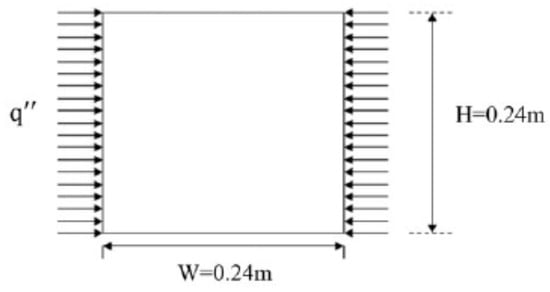
Figure 1.
Schematic of the rectangular square enclosure heated from both sides (reproduced with permission from Ganguli et al. [5]).
1.1. Literature Review
The present section describes prominent studies by different researchers on natural convection in side-heated enclosures. These include types of enclosures, studies on the effect of boundary conditions, working fluids considered inside enclosures, different numerical schemes to solve differential equations, and the development of analytical expressions (also called scaling laws) to describe transient flow behavior. In this section, a comprehensive review of the literature on differentially heated enclosures is presented. This includes studies on i. flow patterns and heat transfer (including experimental and numerical work) and ii. the development of scaling laws (analytical expressions to describe transient length and time scales) and progress in deep learning on such problems. In the changing world of AI, the integration of physics of phenomena and AI is inevitable; hence, understanding the literature on both aspects individually is vital before integration of the two. Most studies related to side-heated enclosures have been confined to differential heating, with one side heated and the other cooled at a constant temperature to maintain a specified temperature gradient. The Rayleigh number (Ra) and Aspect Ratio (height-to-width ratio, AR) are dimensionless parameters important for predicting the heat transfer coefficient. The three are related by empirical correlations of the Nusselt number (Nu) as a function of Ra and AR [6,7,8,9,10,11,12]. Other applications include porous enclosures like thermal insulation, grain storage drying, thermal energy storage, and geological storage of CO2 [13]. Other differentially heated enclosures include non-square shapes (triangular, trapezoidal, rhombic, or parallelogrammical enclosures). They are used in food processing, material processing and nuclear industries. The prime dimensionless parameters include the Darcy number, Rayleigh number, Fourier number, Aspect Ratio, and porosity.
Other engineering applications of natural convection in enclosures include cryogenic tanks, electrical and electronic equipment, materials processing, nuclear safety systems, and chemical process equipment, like crystallization equipment, where crystal growth is essential [14]. In the past decade, applications with enclosures consisting of nanofluids have come up with mixtures of nanoparticles with water. These fluids alter the physical and thermal properties like viscosity and thermal conductivity. The non-dimensional parameters include the Hartman number (Ha), Rayleigh number, and Lewis number (Le). The methods used to solve them are the Eulerian–Eulerian Model (EEM) and the Lattice Boltzmann Model (LBM) [15].
Studies on differentially heated enclosures of different shapes include circular enclosures [16,17,18], inclined enclosures [19,20], rectangular enclosures [21,22], rhombic enclosures [23,24], square enclosures [25,26], triangular enclosures [27,28,29,30], trapezoidal enclosures [31,32], and other complexly shaped enclosures [33,34,35,36]. Different transient flow patterns characterize these enclosures while attaining a steady state. The forthcoming text has elaborated on a few predominant studies related to square/cubical enclosures (not restricted to differential side heating) involving fluid dynamics and heat transfer for different boundary conditions and working fluids.
1.1.1. Effect of Working Fluids and Boundary Conditions on Flow Behavior and Heat Transfer
Arpino, et al. [37] carried out numerical investigations for Ra~108. The significant finding of this research was that higher Ra (~108) significant source terms in governing equations caused numerical instability, and measures to maintain stability needed to be ensured. The authors provided benchmark solutions for differentially heated enclosures, which are essential for studying such problems. Kürekci and Özcan [38] have conducted experimental and numerical investigations in a cubical enclosure for laminar natural convection with air. Experimental investigations were carried out using Particle Image velocimetry (PIV) and CFD simulations using Ansys Fluent with Ra = 1.3 × 10⁷. The authors concluded that the velocity field near the heated and cooled vertical walls was not sensitive to the boundary conditions of the remaining four walls. Armfield, et al. [39] numerically investigated the flow patterns and heat transfer in an inclined differentially heated square enclosure. The enclosure’s lower and upper walls were at adiabatic conditions. The left-side wall is kept at a higher temperature (heated wall) compared to the right-side (cooled) wall for water as working fluid and Ra = 1 × 10⁸. The transient flow patterns in the form of qualitative figures and an empirical correlation for Nu using the predicted data were reported. An important finding was an unconventional variation in Nu for Inclined Enclosures, and a constant value of Nu = 76 for a non-inclined enclosure. Dou and Jiang [40] conducted numerical studies in a differentially heated rectangular enclosure (AR = 0.24) with fins to find the effect number of fins on heat transfer enhancement for a particular Ra range. The authors observed that a single fin on the heated wall caused no heat transfer enhancement for a particular Ra range (3.38 × 10⁵ ≤ Ra ≤ 3.38 × 10⁶). At the same time, there was an exponential increase in heat transfer for a higher Ra range (3.38 × 10⁵ ≤ Ra ≤ 3.38 × 10⁶). The authors attributed this exponential increase in heat transfer to two factors, namely (a) convection domination over conduction as Ra increased from a lower Ra to a higher Ra and (b) induction of flow instability resulting in the rapid increase in heat transfer with the increase in Ra. Mahdavi, et al. [41] conducted experimental and numerical investigations in a cubical enclosure with three different fluids: air, water, and a Water–Ethylene Glycol (EG) mixture to find the nature of flow in the enclosure with Ra numbers of 108 AR around one for a differentially heated enclosure. The authors observed a strong effect of the type of fluid on the hydrodynamics due to the viscosity of fluids. For example, mixing a high viscosity fluid like EG in water provided better uniformity than water when Ra = 108. Further, for a very low viscosity fluid like air, the near-wall profiles were linear in contrast to non-linear profiles for liquids like water. Williamson, et al. [42] numerically investigated the natural convection flow within an inclined differentially heated enclosure with water as a working fluid and heating at the bottom and cooling at the top. The inclination angle was varied from 0° to 90° (Ra = 104 to 108). The authors concluded Nu number was a function of the inclination angle and the Ra number and proposed and empirical correlation obtained from their data. Karatas and Derbentli [43], who used periodic boundary conditions on the heated side of the enclosure, found an increase in the heat transfer rate. Huerta, et al. [44] studied the effect of an obstacle in the middle of the enclosure and found that the overall heat transfer increases with the presence of the obstacle since stratification was restricted and enhanced mixing took place. Several numerical studies have been performed on side-heated enclosures having transient hydrodynamics and heat transfer. These studies had different working fluids and boundary conditions and operated in turbulent regimes with an Ra higher than 1012 [45,46,47,48,49,50,51,52,53,54,55,56]. Since the present study is restricted to laminar flow in natural convection, the above studies have not been mentioned in detail in the present work. Details of the various research works have been presented in Table 1.

Table 1.
Details of dimensionless numbers, geometry, type of geometry, and correlations by different authors.
1.1.2. Status of Available Scaling Laws to Determine Length, Velocity, and Time Scales During Transient Dynamics in an Enclosure
Scaling laws for length, time, and velocity are particularly important due to the interesting phenomena-like oscillations due to the intrusion layer and motion in the core of the enclosure. The discussion in this section typically revolves around researchers comparing experimental and numerical studies expressing different opinions on the motion in the core in the enclosure. Patterson and Imberger [6] conducted numerical simulations and analytical studies before presenting a scaling analysis on length, velocity, and time scales. They established a classification of flow patterns in a differentially heated two-dimensional (2-D) enclosure. They proposed analytical expressions for the three scales (length, velocity, and time) using three parameters: Rayleigh number (Ra), Prandtl number (Pr), and Aspect Ratio (AR). In this classical analysis, the authors suggest that a wide range of Rayleigh numbers (0.1 ≤ Ra ≤ 1011) and the Aspect Ratio, time, length, and velocity scales can be expressed in terms of analytical expressions. In their analysis, Patterson and Imberger [6] predicted time, length, and velocity scales for boundary layers in the regions next to the heated and cooled walls in addition to the intrusion layers that result from the discharge of the boundary-layer flows into the enclosure. The authors concluded that if the Ra, AR, and Pr of the fluid are kept constant, the change in the mode of heat transfer from conduction in enclosures to convection could be represented by time scales, which were a function of two non-dimensional quantities (namely, Ra and AR). Further, the authors also showed that the time scales predicted by the expressions involving the two non-dimensional numbers can represent different flow patterns (or flow regimes) before they attain their final steady state. The time scales also have substantial significance for cases where the time required to attain a steady state is extensive, and the variation in heat transfer is transient.
Ivey [8] conducted laboratory experiments to study the flow patterns occurring in differentially heated square enclosures. In his investigation, the author found the transient oscillatory pattern of the fluid till it reached the final steady state. The authors attributed their observations to the flow’s inertia in the enclosure’s corner regions, which gave rise to hydraulic jumps with associated mixing, which were not observed in the numerical simulations of Patterson [9]. Kimura and Bejan [69] conducted a scaling analysis for natural convection in an enclosure with two ARs (AR = 1 and AR = 2) and Pr = 7. On heated and cooled sides, constant heat flux was kept as boundary conditions. The authors derived scaling laws for length, velocity, and time scales, including the temperature gradient in the core of the enclosure. Equations (1)–(5) given below are provided to present these scaling laws.
Patterson and Armfield [12] did a comprehensive experimental and numerical study to understand the fluid dynamics in a differentially heated square enclosure and contradicted the observations by Ivey [8], who observed no motion in the core. The observations of the authors were however aligned with the observations of Schladow, Patterson and Street [10]. Research on scaling analysis did not receive significant attention for more than two decades after the work of Patterson and Armfield [12], after which Kouroudis, Saliakellis and Yiantsios [70] conducted numerical investigations for natural convection in a square enclosure with high Ra numbers (2.9 × 10¹¹ ≤ Ra ≤ 4 × 10¹⁴) and defined the scaling analysis for the oscillatory nature of waves. Kouroudis, Saliakellis and Yiantsios [70] has clearly investigated that instability occurs for Ra higher than 1012 for enclosures in which both vertical walls are heated in contrast to the differentially heated enclosures, where one vertical wall is heated while the other is cooled. The authors claimed that until the Ra number upto 1012 flows were laminar. Further, the authors did a scaling analysis to remove the dependence of stratification on a number.
Liu, Bian, Zhao, Zhang and Suo [64] carried out numerical studies for a differentially heated enclosure by imposing a linear variation in temperature instead of a constant temperature boundary condition at the side walls. The authors found significant changes in the velocity and temperature patterns and suggested four regimes. Two of these regimes were dominated by viscous buoyancy, while the other two were dominated by inertial buoyancy. The authors also defined the corresponding velocity and temperature scales for an Ra range (1.84 × 10⁷ ≤ Ra ≤ 1.84 × 10¹⁰) using six different Pr numbers (in range Pr = 1–53). The scaling analysis comprised expressions for the thermal boundary layer, the intrusion layer (hydrodynamic and thermal propagation), and the velocity boundary layer. Interesting boundary layer growth characteristics were observed when linear temperature profiles were imposed. These included the two-dimensional nature of the growth of the thermal layer during the start, unlike conventional side-heated enclosures, which are characterized by a temperature jump during the transition to a steady state. Since the scaling laws derived in this work are different than the ones enumerated in Equations (1)–(5), they are given below.
Another study on the effect of boundary conditions on flow patterns was carried out by Chakkingal, Kenjereš, Dadavi, Tummers and Kleijn [65] by imposing sinusoidal temperature wall boundary conditions. The authors chose two factors, namely, the amplitude and the phase angle fluid flow, temperature distribution, and overall heat transfer coefficient. A significant heat transfer enhancement was observed for the Ra number range (Ra = 105–107) with the maximum and minimum values for a number at 00 and 900 phase angle, respectively. Empirical correlations for the nu number relating Ra and the phase angle were developed by regressing the simulation data. Le Quéré [68] conducted numerical investigations in a differentially side-heated enclosure with uniform heat flux boundary conditions for both heating and cooling on the sides with a significantly different approach to study the transition to turbulence. In his investigation, Le Quéré [68] has mentioned that the instabilities started after 1012. During the transition, the flows were essentially unstable. The conventional approach [46,47,48] relied on performing simulations with an initial condition obtained from simulating the same geometry at a lower Ra number. This approach involved a higher time and gave reasonable accuracy. The authors used a different simplified approach to solve such problems to redefine the accuracy and reduce the time taken. The author undertook simulations of steady-state flows for Ra numbers without initial condition solutions irrespective of the stability of the flows for Ra numbers. The authors reported that they could capture the temperature gradient in the core of the enclosure, which was responsible for the unstable nature of higher Ra numbers. The authors further went on to derive scaling laws analytically and to represent this temperature gradient and compare it with their simulation results. The scaling law is given below:
1.1.3. Research Gaps in Previous Work and Motivation and Objectives for the Present Work
The literature review from Section 1.1.2 and Section 1.1.3 suggests that the following gaps are identified in the research of differentially heated enclosures: (1) the Ra range Ra = 107–108 can be considered high for the transition from laminar to turbulence for gases like air as a working fluid. However, quite a few research works have shown that turbulence occurs after Ra = 1012, and hence, an Ra = 1012 and lower could be considered a laminar regime [68,70]. (2) Most works use air as the working fluid while a few works have used liquids like water, water–ethyl glycol mixtures, or nanofluids. (3) Scaling laws that determine the length, velocity, and time scales of transient behavior were of interest four decades ago, but they have remained relatively dormant for two decades and have seen a new surge in the past decade until the present. (4) The class of problems having both sides heated by constant heat flux has not received enough attention. The only studies carried out are for thermal stratification in cryogenic tanks [3,71] and Advanced Heavy Water Reactors (AHWRs) for different Ra, AR, and boundary conditions like both sides heated at a constant temperature or constant heat flux [72]. (5) Thermal stratification in cryogenic tanks in low-gravity environments (especially in space) might occur due to the different boundary conditions of both tank side walls being subject to constant heat flux. Understanding temperature distribution is vital for proper pressure control and safety in such problems. Further, sealed liquid hydrogen vessels in satellite launches involve thermal stratification because both walls are in constant heat flux. This causes corrosion in transport pumps or hydrogen injection into engines where severe stratification has occurred [3]. Very few correlations for Nu for higher Ra have been reported in the literature with liquids as working fluids, even for differentially heated enclosures. The Nusselt number correlation has been proposed by [61] for a wide range of Ra (103 ≤ Ra ≤ 108). However, the correlation is valid for higher ARs (AR > 5) and lower ranges of Ra (Ra < 108) with air as the working fluid. (7) A limited number of studies in differentially heated enclosures have considered Ra in the range 1010–1012 with liquids as working fluids. (8) Heat transfer analysis regarding the Nu number has not been extensively studied for higher Ra numbers for AR of unity and Pr = 7. (9) CFD simulations for such transient flows take a long time while DL models are able to reduce the time by an order of magnitude [5]. Very few efforts have been made in this direction to integrate AI to improve the understanding of spatio-temporal flows.
The motivation behind this work was to ask ourselves a few questions and define objectives towards advancing a step forward. The questions were as follows: i. Can the present analytical expressions predict the phenomena of both-side-heated enclosures? ii. How do the flow physics of both-side-heated enclosures differ from differentially side-heated enclosures? iii. How can CFD help in understanding the flow physics? and iv. How and which DL models trained using CFD data can help in predicting the length and time scales? Based on the above questions, the objectives of the present work were defined as follows: (a) carry out numerical investigations for the both-side-heated enclosure and higher Rayleigh numbers with water as a working fluid (for a heat flux of 500 W/m2 and Ra = 3.7 × 10¹⁰) using inhouse and commercial codes and validate them with experimental data from the literature; (b) develop and integrate a DL model based on the POD-LSTM framework to reduce the time required for the spatial-temporal predictions of CFD simulations; and (c) perform heat transfer analysis and develop a Nu number correlation as a function of Ra for the prediction of heat transfer coefficients for the both-side-heated enclosure.
2. Mathematical Expressions and Methodology Adopted for CFD and Deep Learning Models
2.1. Mathematical Modeling
2.1.1. Governing Equations
For developing an inhouse CFD Fortran code, the 2-D conservation equations governing the mass, momentum, and energy of natural convection in a heated enclosure are given by Equations (15)–(18). The fluid is assumed incompressible with the Boussinesq approximation to incorporate buoyancy effects. Viscous dissipation is neglected in the energy balance equation.
Continuity equation
X-momentum equation
Y-momentum equation
Energy equation
The Rayleigh number, (Ra), based on the heat flux (given by Equation (19)) is as below.
Fluid properties are at an average temperature of 310 K, with a heat flux of 500 W/m2 and an AR of 1. In the reported literature, [4] ΔT has been measured experimentally as a difference between the highest wall temperature and the coldest water temperature in the tank’s core. In this case (termed Case 1), the measured ΔT is 3 °C with the corresponding heat flux of 500 W/m2.
2.1.2. Boundary Conditions for CFD Simulations
The heat transfer coefficient (h) was considered as 10 W/m2K.
All boundary conditions are given by Equations (20)–(23) for both the inhouse code and the commercial software.
2.2. Methodology for CFD Simulations
2.2.1. Inhouse Code
The natural convection inside the tank is simulated by numerically solving the Navier–Stokes (N-S) equations of continuity, momentum, energy, and boundary and initial conditions. An appropriate pressure-based finite volume method (FVM) was used with pressure velocity coupling achieved by the SIMPLE algorithm. The momentum and energy equations were solved using the Second Order Upwind (SOD) method. The trigonal matrix algorithm (TDMA) was used to solve simultaneous equations. The relaxation factors of 0.3 were used for pressure equations and 0.7 were used for momentum equations, while 0.6 for energy equations was used. A relaxation factor of 0.5 was used for solving the pressure. The residuals were 1 × 10⁻⁴, 1 × 10⁻⁶, and 1 × 10⁻⁸ for pressure, momentum, and energy equations.
2.2.2. Commercial Code
Due to the availability of better numerical schemes in commercial software, they have been used wherever necessary. Higher order schemes like the fourth order QUICK scheme were used to solve energy equations, while the PISO scheme was used for pressure equations. The relaxation factors and residuals were kept the same in both cases. An Intel 2 GHz Core™2 Duo processor was used for this purpose.
2.3. Grid Sensitivity for Ensuring the Best Grid for CFD Simulations
The grids used were the same as our previous work of [5] and have been reproduced in Figure 2.
Figure 2.
Details of the mesh used for commercial code (reproduced with permission from Ganguli, Tabib, Deshpande and Raval [5]).
However, a grid sensitivity graph (at the time when the system reached steady state) has been presented to test the inhouse code results. Figure 3i–iv shows the grid sensitivity at a dimensionless time of 0.011 when the system has reached a steady state. A 7% deviation is observed between the first two grids (denoted by (A) and (B) in the figures). Meanwhile, a 2.5% deviation has been observed between the second and third grids. The results were similar for both the inhouse and the commercial code (Ansys Fluent 18.1) used for the analysis. Figure 4 shows the geometry and the selected mesh for the study.
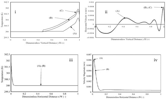
Figure 3.
Grid sensitivity for a constant heat flux of 500 W/m2 applied on both vertical sides of enclosure at t = 540 s. (i) Vertical Central Temperature Profile, (ii) Vertical Central Horizontal Velocity Profile, (iii) Horizontal Central Temperature Profile, and (iv) Horizontal Central Velocity Magnitude Profile for (A) Non-uniform Grid Size = 101 × 101, (B) Non-uniform Grid Size = 141 × 141, and (C) Non-uniform Grid Size = 181 × 181 for commercial code. (Figures (iii) and (iv) have been reproduced with permission from Ganguli, Tabib, Deshpande and Raval [5]).
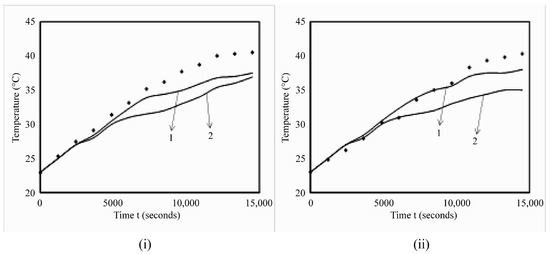
Figure 4.
Quantitative analysis of commercial and inhouse codes with experimental results. (i) Transient centerline axial temperature profiles; (ii) transient wall averaged temperature profiles. Lines represent simulation results. 1. Commercial code; 2. Inhouse code. Symbols represent experimental results (reproduced with permission from Ganguli, Tabib, Deshpande and Raval [5]).
2.4. Deep Learning (DL) Model
The DL model of [5] has been used. The model is described in brief below to give the reader a glimpse of the model. A Nonintrusive Reduced Order Modeling (NIROM) methodology referred to as the POD-LSTM framework for predicting the flow fields at different times. A solely data-driven neural network approach is used to predict the time coefficients. The snapshot data obtained from the CFD simulations undergoes a POD transform and provides us with the time-dependent modal coefficients essential to temperature or velocity time series data. The methodology comprises a computationally heavy offline training phase to build the POD-LSTM framework and an efficient online phase for reconstructing flow fields for valid particularization of the parameters. In the offline phase, the POD-LSTM framework is trained with a flow and temperature field database, while in the online phase, the fields are reconstructed.
3. Results
The present section focuses on the understanding of the key physics of the problem, i.e., dimensional and dimensionless time analysis using the results of the full order model and comparing them with the other analytical models. Further, the section presents the flow patterns and transient temperature profiles for the heat flux of 500 W/m2 and flow patterns of 1000 W/m2. The DL model is trained and tested for Ra (Ra = 6.55 × 10¹⁰), and the results have been compared with the CFD data.
Dimensionless time analysis (as of Patterson and Imberger [6]) has been used to understand the transient flow patterns. It has been observed that the velocity patterns are dominant in the upper layer (3 cm from the top layer) after t’ = 0.031 non-dimensional time units. The steady state is, however, achieved after t′ = 0.31 non-dimensional time units.
3.1. Model Validation
An inhouse code has been developed not only for research but also for educating the undergraduates about challenges in code development. Quantitative plots of temperature profiles (center line given by Figure 4 (i) and wall averaged given by 4(ii)) comparing predictions of codes with the experimental results of Das, Chakraborty and Dutta [4] are shown in Figure 4. Both codes match the temperature profiles well until the time of 5000 s, after which, a deviation of 8% is observed for the commercial code for the centerline temperature profile, while a deviation around 15% is observed for the inhouse code. The deviations of commercial code may be attributed to the fact that the experimental setup is three-dimensional while the CFD simulations are in two dimensions. The higher deviations in the inhouse code are attributed to lower-order numerical simulation schemes. The commercial code predicts the wall temperatures with a deviation of 6% after 12,000 s, while it almost matches the wall temperatures until 12,000 s. However, the inhouse code shows higher deviations in prediction of the wall temperature with a deviation of 8–10% after 5000 s. This is attributed to the higher-order schemes used for the commercial codes compared to the inhouse code. As per the model validation, the commercial code is selected for the further analysis of results in the forthcoming sections.
3.2. Flow Patterns
This subsection focuses on the physics of flow and how dimensionless scaling analysis is important to describe flow physics. In this section, we describe the development of flow and temperature patterns from initial thermal and velocity boundary layer formations to the movement of the boundary layers across horizontal and vertical directions across different parts of the enclosure.
3.2.1. Scaling Analysis of Time Scales Using CFD During Development of Boundary Layer
The typical sequence of flow involves the development of intrusion of the thermal boundary layers from the two side walls towards the center, moving the intrusion layers downwards and back to the square wall, development and movement of the velocity boundary layers, and finally, the role of boundary layers in transferring the heat to the center or core of the enclosure. The dimensionless time (t′ where t′ = Ut/L), the dimensional time t, and the sequence of flow patterns is given in Table 2.
Table 2.
Transient Flow Phenomena occurring for both sides of the heated enclosure at a constant heat flux of 500 W/m2.
3.2.2. Qualitative Flow Patterns for Ra = 3.27 × 10¹⁰
Figure 5, Figure 6, Figure 7, Figure 8, Figure 9 and Figure 10 show the velocity and temperature contours for Ra = 3.27 × 10¹⁰. The downward movement of the velocity boundary layer and the advancement of the thermal boundary layer (or intrusion layer) intruding the top fluid layer in a horizontal direction can be observed at t = 20 (Figure 5A,B). The upward movement of the velocity boundary layer continues at t = 40 s (Figure 6A), while an inverted U-shaped pattern near the upper horizontal wall can be observed in Figure 6B.
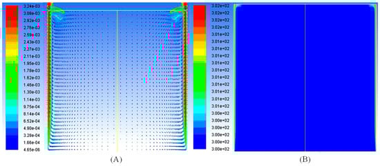
Figure 5.
For a constant heat flux from both sides at time t = 20 s: (A) Velocity Vector; (B) Temperature Contour.
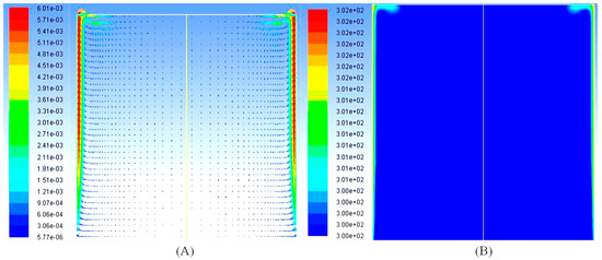
Figure 6.
For a constant heat flux from both sides at time t = 40 s: (A) Velocity Vector; (B) Temperature Contour.
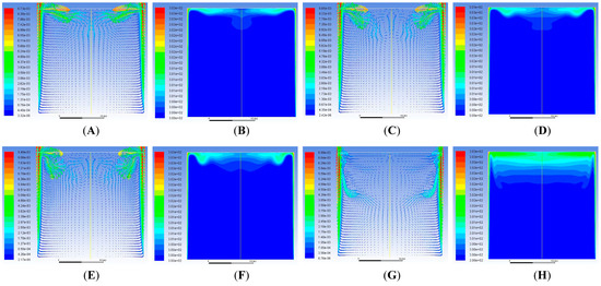
Figure 7.
For a constant heat flux from both sides at time t = 75 s: (A) Velocity Vector and (B) Temperature Contour; t = 90 s: (C) Velocity Vector and (D) Temperature Contour; t = 100 s: (E) Velocity Vector and (F) Temperature Contour; and t = 120 s: (G) Velocity Vector and (H) Temperature Contour. (Reproduced with permission from Ganguli, Tabib, Deshpande and Raval [5]).
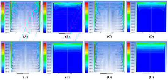
Figure 8.
For a constant heat flux from both sides at time t = 150 s: (A) Velocity Vector and (B) Temperature Contour; t = 180 s: (C) Velocity Vector and (D) Temperature Contour; t = 250 s: (E) Velocity Vector and (F) Temperature Contour; and t = 300 s: (G) Velocity Vector and (H) Temperature Contour.
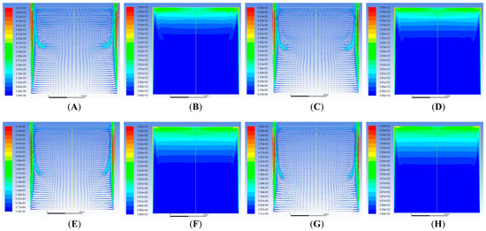
Figure 9.
For a constant heat flux from both sides at time t = 350 s: (A) Velocity Vector and (B) Temperature Contour; t = 400 s: (C) Velocity Vector and (D) Temperature Contour; t = 550 s: (E) Velocity Vector and (F) Temperature Contour; and t = 620 s: (G) Velocity Vector and (H) Temperature Contour.
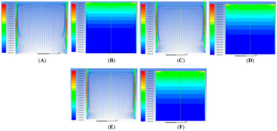
Figure 10.
For a constant heat flux from both sides at time t = 1000 s: (A) Velocity Vector and (B) Temperature Contour; t = 1280 s: (C) Velocity Vector and (D) Temperature Contour; and t = 1380 s: (E) Velocity Vector and (F) Temperature Contour.
Figure 7A,B shows the increase in the intrusion length of the velocity boundary layers and their corresponding merging at the top center of the enclosure. The velocity magnitudes in the intrusion layers are 50% less than those in the wall boundary layers. The movement of velocities are up to only 15–20% of the top portion of the enclosure. Figure 7C shows velocity vectors moving towards the center and starting to form cellular structures. Figure 7D shows the discharge of heat from thermal boundary layers to the center. The description is also written in Table 2.
Two small circulation cells are observed on the top left and right corners and two large counter-rotating cells at the upper central region, as observed in Figure 7E. The thermal boundary layers near the corners show a dip at the corner, signifying retardation of the boundary layer (Figure 7F). This corresponds to the time and phenomena tabulated in Table 2. Further, Figure 7G,H show the movement of the circulating cells and thermal boundary layers, as described in Table 2.
The phenomena of both velocity and temperature are described in detail in Figure 8 and Figure 9 in the forthcoming paragraphs. Figure 8A shows the velocity vectors at t = 150 s. Surprisingly, the two central counter-rotating rolls at the center are shorter and more comprehensive than earlier. Here, we restrict our discussion to the movement of rolls only, rather than discussing the strength of these rolls, which is out of the scope of the current objective of the present work. Furthermore, there are smaller rolls near the top corners of the enclosure (at the place where the thermal boundary layer discharges). A closer look at the velocity vectors shows the fluid particles moving towards the bottom.
In contrast, a smaller circulation from the center to the bottom of the wall is observed. At the same time, the rest of the enclosure is still stagnant. This ascertains that the intense hydrodynamic effects are limited to the upper part of the enclosure and near the walls at the bottom. The temperature contours at a particular time instant are depicted in Figure 6 (B), which shows thicker intrusion thermal boundary layers compared to those depicted earlier. These also show an increase in the extent of stratification.
Figure 8C,D depict results similar to that of Figure 8A,B at different times with heat discharge to the central portion of the enclosure by the fluid particle movement due to the velocity intrusion boundary layer in the downward direction. The thermal boundary intrusion layer contributes to a steeper vertical gradient downwards.
Figure 8E depicts the movement of the velocity intrusion layer further downward vertically, contributing to discharge inside the enclosure. Similarly, in Figure 8F, it can be observed that the vertical thermal gradients move further down compared to the previous times, as depicted in Figure 5 and Figure 6.
Figure 8G shows the weakening of the discharge of the velocity boundary layer, with the intrusion layer responsible for the discharge becoming thin. A low-velocity zone is formed at the center below the top portion. It is concentrated around 10% of the area of the enclosure. This is due to the low-pressure zone formed in the region where the fluid elements start moving from the sides towards the lower part of the enclosure.
Figure 9A,C show the discharge into the enclosure due to the velocity intrusion layer. The intrusion layer divides the enclosure’s flow field into two halves, with lower velocities in the top portion and higher velocities rushing through the intrusion layers into the bottom of the enclosure. From Figure 9B,D, it can be observed that the thermal gradients move vertically downward, stratifying 25% of the enclosure with vertical temperature gradients and thermal intrusion layers acting as the source for such temperature gradients.
Figure 9E,G show that the thermal discharge continues to the bottom of the enclosure. At the same time, the movement of the fluid particles is restricted to the top 5% of the enclosure, with the rest of the top part having a constant flow pattern. Thermal gradients, however, continue to increase downwards, as depicted in Figure 9F,H.
Figure 10 shows that the velocities have a stagnant velocity pattern across the entire enclosure except for the top 5% area near the surface, where there is a zig-zag pattern of top-layer velocities. Velocities at the top surface turn, and the fluid starts a downward vertical motion towards the bottom of the enclosure.
As we move ahead in time, the entire enclosure has a thermal gradient. At the same time, the zig-zag pattern of velocity vectors is restricted to the top portion only, and the magnitude of temperatures and velocities increases, eventually reaching a steady state.
The simulations were carried out for 15,000 s to match the time for which the experimental investigations in the literature were carried out. The final flow patterns reported in the literature were also observed in the simulations, confirming the model’s robustness.
3.2.3. Qualitative Flow Patterns for Ra = 6.55 × 10¹⁰
Figure 11A–L show the velocity vectors and temperature contours for different time intervals. Interestingly, a comparison of the patterns for a heat flux of 500 W/m2 with 1000 W/m2 shows that both the patterns (velocity and temperatures) are similar for both heat fluxes. The magnitudes are higher for 1000 W/m2, but the trends are the same. In fact, the phenomena of the intrusion layer movement were at exactly the same time. The position of the circulation cells is also similar, with the strength being higher in the case of 1000 W/m2.
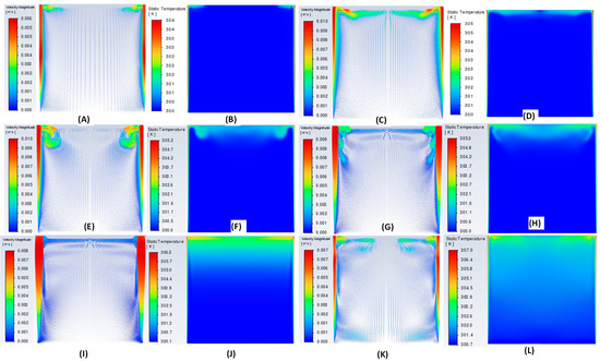
Figure 11.
For a constant heat flux of 1000 W/m2 from both sides at time t = 40 s: (A) Velocity Vector and (B) Temperature Contour; t = 75 s: (C) Velocity Vector and (D) Temperature Contour; t = 120 s: (E) Velocity Vector and (F) Temperature Contour; t = 180 s: (G) Velocity Vector and (H) Temperature Contour; t = 400 s: (I) Velocity Vector and (J) Temperature Contour; and t = 1000 s: (K) Velocity Vector and (L) Temperature Contour.
The equations for length, velocity, and time scales reported in the literature (defined as scaling laws) have been tabulated in Table 3. For the present work, the calculated magnitudes (as per the expressions) of these parameters using the given equations have also been included and compared with the magnitudes obtained from CFD simulations. The analysis of [6] is based on the differentially heated enclosure, where a constant temperature is maintained on both sides (one heated and the other cooled). In ref. [57]’s analysis, one wall was heated using constant heat flux. At the same time, the other was maintained at a constant temperature. The present work has both walls heated using a constant heat flux. Hence, the predicted results showed different flow patterns from both analyses. It is evident that the mechanism of the (a) intrusion layer formation (b) meeting the two intrusions layers from side walls to the center and the discharge of heat into the enclosure would have different magnitudes of the length, velocity, and time scales than the analytical expressions. However, the values for the time scales of the boundary layer formation and intrusion layer arrival time thicknesses of both the thermal and hydrodynamic boundary layers are closer to the analysis of Poujol, Rojas and Ramos [57] than that of Patterson and Imberger [6]. The reasons for this are due to the formulation of analytical expressions and the physics of the phenomena. The former is attributed to two factors: (1) due to their modification of analytical expressions (that were derived by Patterson and Imberger [6] and Poujol, Rojas and Ramos [57]) to incorporate constant flux boundary conditions and (2) a viscous fluid (having Pr = 220) used as the working fluid by Poujol, Rojas and Ramos [57].
Table 3.
Comparison of scaling analysis predicted with CFD predictions of present work.
In terms of the physics of the phenomena, the explanation is as follows: (a) in a both-side-heated enclosure, there is no heat sink, and the fluid near both walls becomes lighter and moves up. The heat is removed from the hot wall due to the cold fluid moving down in a differentially heated case, which is not present in both-side-heated cases. Further, the fluid is being swept away from the hot and cold wall in case of a differentially heated case, reducing the thickness of the boundary layer. Due to this, the thickness of the thermal boundary layer on both sides of the heated case is nearly double that in a differential-heated case with the same Ra number and Aspect Ratio. (b) It is also important to note that the velocities in the thermal boundary layer are low since there is no recirculation due to the hot and cold wall combination, as in a differentially heated case. Firstly, the resistance is high due to higher boundary layer thickness, causing the fluid elements in the boundary layer to move slowly. Hence, it can be observed that the velocities in the present case are more than an order of magnitude lower than a differentially heated case. (c) Due to the lower velocities and higher fluid resistance due to the non-sweeping of the fluid, the velocity boundary layer thickness and the intrusion layer thickness in the present case are also higher than that in a differentially heated case. (d) The arrival time of the intrusion layer, however, is lower in both the case of Patterson and Imberger [6] and as compared to the present work, which is due to the resistance offered by the higher boundary layer thicknesses for both the velocity and thermal boundary layers, causing slower movement of the intrusion layer as compared to the differentially heated case. The values of [57] for the intrusion layer thickness are closer to the present work due to the viscous fluid considered by the authors.
While the recent scaling laws by a few researchers [64,68] have been included, comparing CFD results has been restricted to only two authors to avoid confusion. This also requires a more detailed analysis and study, which is out of the scope of the present work.
3.3. Heat Transfer
The heat transfer across the enclosure has been calculated using the Nusselt number. The Nusselt number is given by Equation (24), as shown below.
Tcl is the average temperature of the vertical centerline at a pseudo-steady state, and Th is the average wall temperature at a pseudo-stable state. The above equation and the temperature difference were deduced from [4]. CFD simulations were carried out for different heat fluxes for the Ra range (Ra = 1.31 × 10¹⁰–Ra = 6.55 × 10¹⁰). Though the transition to turbulence takes place at Ra = 1 × 10¹², we restrict our analysis to the fact that there is only one experimental data point. The heat flux for the experiments was restricted to 1000 W/m2, which is the maximum Ra number we have chosen.
Figure 12 shows the parity plot of predicted vs. experimental Nu numbers. Correlation for the Nusselt number from the generated data is given by Equation (25) below:
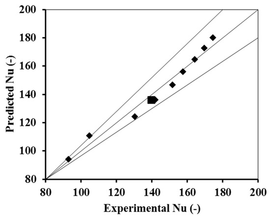
Figure 12.
Parity plot for Nusselt number square symbol represents the experimental point while the rhombus symbol represents prediction based on Equation (25).
The deviation of the predicted results from experimental results is an underprediction of 2%. In comparison, the predictions for other results have an underprediction between 4 and 7%. The correlation is developed for an enclosure with an Aspect Ratio of 1 and the Prandtl number Pr = 7. Since the enclosure is heated from both sides, the literature correlations for differential heating are not chosen. The deviations are due to transient heat transfer from the top of the enclosure. The heat transfer coefficient from the water–liquid interface might be a function of time that has not been considered in the simulations.
3.4. Assessment of POD-LSTM Framework (DL Model)
In this section, the POD-LSTM framework [5,73,74] has been trained and tested for Ra = 6.55 × 10¹⁰. The approach for obtaining the results is similar to that explained in [5]. The Y axis ranges from 0 to 0.24 while X-axis ranges from 0 to 0.12 since only half geometry is simulated due to symmetry.
Figure 13 shows the approximation/reconstruction of the velocity and temperature field for Ra = 6.55 × 10¹⁰, i.e., the POD modes. As shown in Figure 13A, out of the eight modes selected for analysis at t = 100 s, the first four modes contain most of the energy-containing eddies in the top part of the enclosure. Furthermore, the vertical boundary layer near the wall and the intrusion layer at the top are captured qualitatively in all the modes. These results are similar to the lower Ra number results reported in our previous work [5]. Figure 13B shows the corresponding temperature modes in which the first three modes consist of most of the energy. Figure 14A, B show the ones contoured by POD and the reconstructed POD-LSTM framework for five different time instants: 50, 100, 150, 200, and 250 s. It can be observed that the POD-LSTM methodology can capture both the qualitative and quantitative trends in less amount of time than actual CFD simulations.
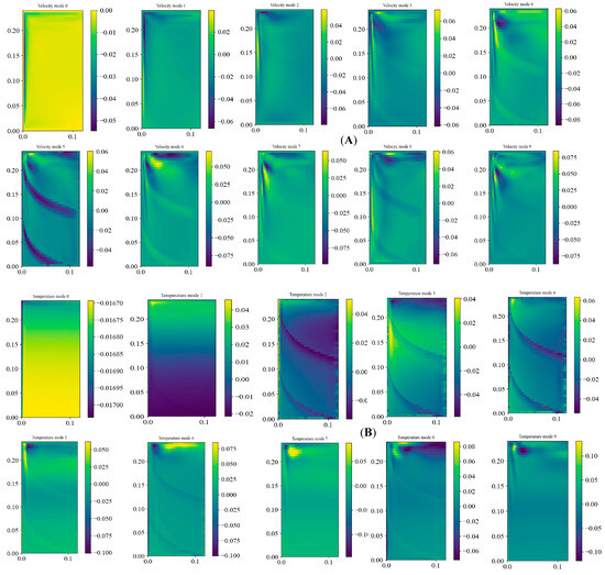
Figure 13.
POD constructed spatial modes at Ra = 6.55× 10⁹ for (A) velocity modes from 0 to 9 and (B) temperature modes from 0 to 9.
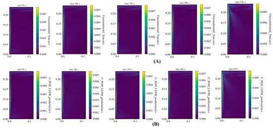
Figure 14.
U velocity contour predictions between (A) POD reconstructed and (B) POD-LSTM framework at 50 s, 100 s, 150 s, 200 s, and 250 s.
In contrast, Figure 15 shows the energy in the velocity basis modes while Figure 13 plots the loss performance of the LSTM model.
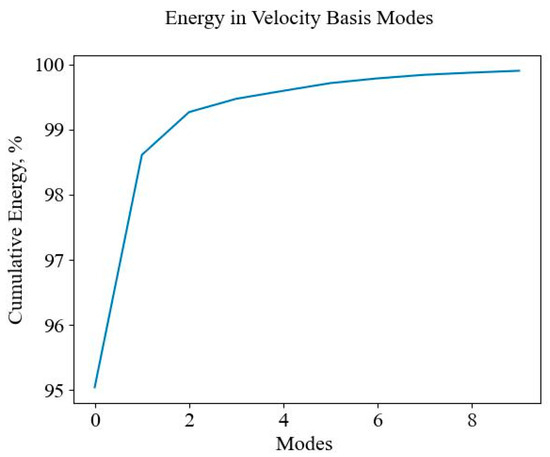
Figure 15.
Energy contained in velocity basis modes.
Figure 16 shows that the training and validation loss trends are the same, and the LSTM performance is good, with a deviation around 4%.
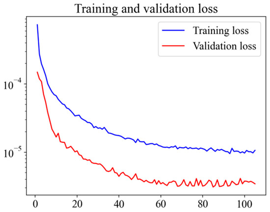
Figure 16.
LSTM’s training and validation loss.
Since most of the dynamics occur within the first 1000 s, the variation in time coefficients with temporal modes has been considered for the first 1000 s. The variation in the time coefficients associated with the spatial modes for the first 250 s is shown in Figure 17. It can be observed that the velocity temporal coefficients 1 to 4 precisely match with the LSTM predicted coefficients. In contrast, the fifth coefficient has a maximum deviation of less than 5%.
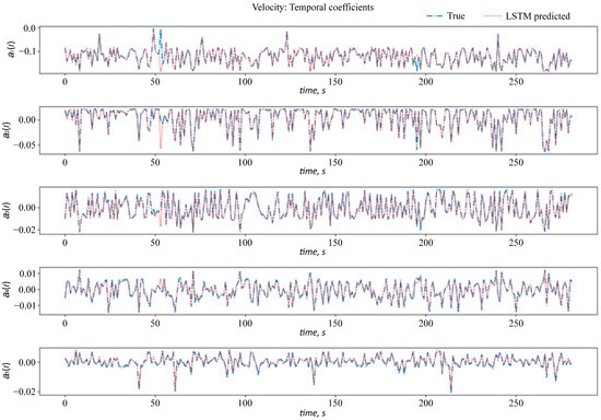
Figure 17.
LSTM predicted temporal coefficients quantities for Ra = 6.55 × 10¹⁰; temporal coefficients for velocity. The blue line represents ground truth data, and the red line represents LSTM predicted data. The first five significant modes are plotted.
Figure 18 A, B shows the velocity and temperature coefficient variation for each of the eight modes with time up to 1000 s. As observed in Figure 18 B, in temperature variations, except mode 2, higher variations for the time duration are not observed. For corresponding velocity modes (Figure 18A), there are huge variations (modes 2 and 3) in the temporal coefficients for velocity modes for the entire 1000 s, while modes 4 to 8 showed variation in first 200 s. So, the POD-LSTM framework has a good scope for continued research as an excellent alternative method to predict transient dynamics on both sides of the heated enclosures.
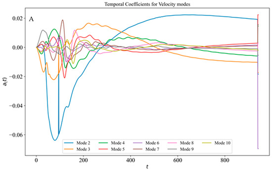
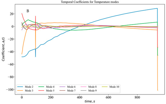
Figure 18.
Variation in temporal coefficients with time for (A) velocity and (B) temperature modes.
4. Conclusions
The following conclusions can be drawn:
- CFD simulations of both-side-heated enclosures for two Ra numbers, Ra = 3.27 × 10¹⁰ and Ra = 6.55 × 10¹⁰, were carried out. Analysis of the scaling analysis for Ra = 3.27 × 10¹⁰ shows that current analytical expressions defined by scaling laws are unable to predict the length and time scales for the Ra number for a both-side-heated enclosure, indicating that these enclosures behave differently than the well-studied differentially heated enclosures.
- The flow patterns in the form of velocity vectors and temperature contours clearly depict that the physics of the phenomena is different than the conventionally studied differentially heated enclosures reported in the literature. The major highlights were the merging of intrusion layers and dynamics of fluid elements near the wall as well as in the bulk.
- The predicted flow pattern for the commercial code shows good qualitative and quantitative agreement with the experimental results in the literature. The inhouse code, however, has a higher deviation and needs improvement.
- A new empirical correlation of Nusselt number with Ra number has been developed for an Ra range of 1.3 × 10¹⁰–6.55 × 10¹⁰. The predictions are in good agreement with the experimental values from the literature [4].
- CFD simulations required a large amount of time and computational power to simulate such transient phenomena. Alterative, fast models are necessary to simulate such phenomena.
- The DL Model consisting of the POD-LSTM framework is able to predict the temporal dynamics of the velocity with very good accuracy and takes at least an order of magnitude less time than for a full CFD simulation.
- The present study also presents studies with their own code, which, after improvisations, can be used for integrating CFD and DL models for the fundamental understanding of transient flows for both-side-heated enclosures.
- The present study gives a new dimension to the research on side-heated enclosures in terms of qualitative and quantitative analysis and can be used for different applications.
5. Future Work
The present work would be extended to incorporate the Physics Informed Neural Networks (PINNS) for future complex flows, where it would be more advantageous than LSTM.
Author Contributions
Conceptualization, A.A.G.; methodology, A.A.G.; software, A.A.G. and S.S.D.; validation, A.A.G. and S.S.D.; formal analysis, A.A.G.; investigation, A.A.G.; resources, A.A.G. and S.S.D.; data curation, A.A.G.; writing—original draft preparation, A.A.G.; writing—review and editing, A.A.G., S.S.D. and M.S.R.; visualization, A.A.G.; supervision, M.S.R.; project administration, A.A.G.; funding acquisition, A.A.G. All authors have read and agreed to the published version of the manuscript.
Funding
This research received no external funding.
Data Availability Statement
Data is confidential but can be made available for genuine requirements.
Acknowledgments
The authors would like to thank the School of Engineering and Applied Sciences, Ahmedabad University, for the resources provided for the computational work. We also thank M.V. Tabib for his inputs in Machine Learning part.
Conflicts of Interest
The authors declare no conflicts of interest.
Nomenclature
| Alphabetical Letters | ||
| AR | Aspect Ratio | - |
| Height of the Enclosure | m | |
| Length of the enclosure | m | |
| Pressure of the Fluid | Pa | |
| Nu | Nusselt Number | - |
| Prandtl Number | - | |
| Rayleigh Number | - | |
| Temperature of the Fluid | K | |
| Reference Temperature of the Fluid | K | |
| Temperature of the Convection Fluid | K | |
| W | Width of the Enclosure | m |
| Gravitational Acceleration | 9.81 m/s2 | |
| Convection Heat Transfer Coefficient | W/(m2K) | |
| Thermal Conductivity of the Fluid | W/(mK) | |
| Heat Flux | W/m2 | |
| Stratification Factor | K/m | |
| Time | s | |
| t′ | Dimensionless Time | - |
| Horizontal Velocity of the Fluid In Direction | m/s | |
| Vertical Velocity of the Fluid In Direction | m/s | |
| Velocity of the Thermal Boundary Layer | m/s | |
| Horizontal Distance Co-ordinate | m | |
| Vertical Distance Co-ordinate | m | |
| Greek Symbol | ||
| Difference | ||
| Thermal Diffusivity of the Fluid | m2/s | |
| Volumetric Coefficient of Thermal Expansion of the Fluid | K−1 | |
| Thickness of Intrusion Layer | m | |
| Thermal Boundary Layer Thickness | m | |
| Hydrodynamic Boundary Layer Thickness | m | |
| Angle of Inclination | ° | |
| Kinematic Viscosity of the Fluid | m2/s | |
| Density of Fluid | kg/m3 | |
| Time for Thermal Boundary Layer Development | s | |
| Arrival Time of the Intrusion Layer | s | |
| Subscripts | ||
| Intrusion Layer Parameter | ||
| Thermal Layer Parameter | ||
| Hydrodynamic Layer Parameter | ||
| Convection Fluid Parameter | ||
| Reference Parameter | ||
| Upper wall Parameter | ||
| In the Direction of x Co-ordinate | ||
| In the Direction of y Co-ordinate | ||
| In the Direction of z Co-ordinate | ||
| Superscripts | ||
| ′ | Dimensionless Parameter | |
| Heat Input Parameter | ||
| Abbreviations | ||
| 2-D | Two Dimensional | |
| AR | Aspect Ratio | |
| CFD | Computational Fluid Dynamics | |
| DNS | Direct Numerical Simulation | |
| FVM | Finite Volume Method | |
| PISO | Pressure-Implicit with Splitting of Operators | |
| QUICK | Quadratic Upstream Interpolation for Convective Kinematics | |
| SIMPLE | Semi-Implicit Method for Pressure Linked Equations | |
| SOD | Second Order Upwind | |
| TDMA | Tri Diagonal Matrix Algorithm | |
References
- Turner, J. Convection in the mantle: A laboratory model with temperature-dependent viscosity. Earth Planet. Sci. Lett. 1973, 17, 369–374. [Google Scholar] [CrossRef]
- Ostrach, S. Natural convection in enclosures. J. Heat Transfer. 1988, 110, 1175–1190. [Google Scholar] [CrossRef]
- Tanyun, Z.; Zhongping, H.; Li, S. Numerical simulation of thermal stratification in liquid hydrogen. Adv. Cryog. Eng. Part A 1996, 41, 155–161. [Google Scholar]
- Das, S.; Chakraborty, S.; Dutta, P. Natural convection in a two-dimensional enclosure heated symmetrically from both sides. Int. Commun. Heat Mass Transf. 2002, 29, 345–354. [Google Scholar] [CrossRef]
- Ganguli, A.A.; Tabib, M.V.; Deshpande, S.S.; Raval, M.S. Deep learning based hybrid POD-LSTM framework for laminar natural convection flow in a rectangular enclosure. Chem. Prod. Process Model. 2024, 20, 221–239. [Google Scholar] [CrossRef]
- Patterson, J.; Imberger, J. Unsteady natural convection in a rectangular cavity. J. Fluid Mech. 1980, 100, 65–86. [Google Scholar] [CrossRef]
- Yewell, R.; Poulikakos, D.; Bejan, A. Transient natural convection experiments in shallow enclosures. J. Heat Transfer. 1982, 104, 533–538. [Google Scholar] [CrossRef]
- Ivey, G. Experiments on transient natural convection in a cavity. J. Fluid Mech. 1984, 144, 389–401. [Google Scholar] [CrossRef]
- Patterson, J.C. Unsteady natural convection in a cavity with internal heating and cooling. J. Fluid Mech. 1984, 140, 135–151. [Google Scholar] [CrossRef]
- Schladow, S.; Patterson, J.; Street, R. Transient flow in a side-heated cavity at high Rayleigh number: A numerical study. J. Fluid Mech. 1989, 200, 121–148. [Google Scholar] [CrossRef]
- Schladow, S. Oscillatory motion in a side-heated cavity. J. Fluid Mech. 1990, 213, 589–610. [Google Scholar] [CrossRef]
- Patterson, J.C.; Armfield, S. Transient features of natural convection in a cavity. J. Fluid Mech. 1990, 219, 469–497. [Google Scholar] [CrossRef]
- Das, D.; Roy, M.; Basak, T. Studies on natural convection within enclosures of various (non-square) shapes—A review. Int. J. Heat Mass Transf. 2017, 106, 356–406. [Google Scholar] [CrossRef]
- Pimputkar, S.M.; Ostrach, S. Convective effects in crystals grown from melt. J. Cryst. Growth 1981, 55, 614–646. [Google Scholar] [CrossRef]
- Sadeghi, M.S.; Anadalibkhah, N.; Ghasemiasl, R.; Armaghani, T.; Dogonchi, A.S.; Chamkha, A.J.; Ali, H.; Asadi, A. On the natural convection of nanofluids in diverse shapes of enclosures: An exhaustive review. J. Therm. Anal. Calorim. 2020, 147, 1–22. [Google Scholar] [CrossRef]
- Ali, M.; Zeitoun, O.; Almotairi, S. Natural convection heat transfer inside vertical circular enclosure filled with water-based Al2O3 nanofluids. Int. J. Therm. Sci. 2013, 63, 115–124. [Google Scholar] [CrossRef]
- Huminic, G.; Huminic, A. A numerical approach on hybrid nanofluid behavior in laminar duct flow with various cross sections. J. Therm. Anal. Calorim. 2020, 140, 2097–2110. [Google Scholar] [CrossRef]
- Yu, Q.; Lu, Y.; Zhang, C.; Wu, Y.; Sunden, B. Experimental and numerical study of natural convection in bottom-heated cylindrical cavity filled with molten salt nanofluids. J. Therm. Anal. Calorim. 2020, 141, 1207–1219. [Google Scholar] [CrossRef]
- Zhang, R.; Ghasemi, A.; Barzinjy, A.A.; Zareei, M.; Hamad, S.M.; Afrand, M. Simulating natural convection and entropy generation of a nanofluid in an inclined enclosure under an angled magnetic field with a circular fin and radiation effect. J. Therm. Anal. Calorim. 2020, 139, 3803–3816. [Google Scholar] [CrossRef]
- Öğüt, E.B. Natural convection of water-based nanofluids in an inclined enclosure with a heat source. Int. J. Therm. Sci. 2009, 48, 2063–2073. [Google Scholar] [CrossRef]
- Oztop, H.F.; Abu-Nada, E. Numerical study of natural convection in partially heated rectangular enclosures filled with nanofluids. Int. J. Heat Fluid Flow 2008, 29, 1326–1336. [Google Scholar] [CrossRef]
- Esmaeili, H.; Armaghani, T.; Abedini, A.; Pop, I. Turbulent combined forced and natural convection of nanofluid in a 3D rectangular channel using two-phase model approach. J. Therm. Anal. Calorim. 2019, 135, 3247–3257. [Google Scholar] [CrossRef]
- Anandalakshmi, R.; Basak, T. Natural convection in rhombic enclosures with isothermally heated side or bottom wall: Entropy generation analysis. Eur. J. Mech.-B/Fluids 2015, 54, 27–44. [Google Scholar] [CrossRef]
- Dutta, S.; Goswami, N.; Pati, S.; Biswas, A.K. Natural convection heat transfer and entropy generation in a porous rhombic enclosure: Influence of non-uniform heating. J. Therm. Anal. Calorim. 2021, 144, 1493–1515. [Google Scholar] [CrossRef]
- Bhuiyana, A.; Alam, M.S.; Alim, M. Natural convection of water-based nanofluids in a square cavity with partially heated of the bottom wall. Procedia Eng. 2017, 194, 435–441. [Google Scholar] [CrossRef]
- Dahani, Y.; Hasnaoui, M.; Amahmid, A.; Hasnaoui, S. Lattice-Boltzmann modeling of forced convection in a lid-driven square cavity filled with a nanofluid and containing a horizontal thin heater. Energy Procedia 2017, 139, 134–139. [Google Scholar] [CrossRef]
- Salmun, H. Convection patterns in a triangular domain. Int. J. Heat Mass Transf. 1995, 38, 351–362. [Google Scholar] [CrossRef]
- Joudi, K.; Hussein, I.; Farhan, A. Computational model for a prism shaped storage solar collector with a right triangular cross section. Energy Convers. Manag. 2004, 45, 391–409. [Google Scholar] [CrossRef]
- Ridouane, E.H.; Campo, A.; Chang, J.Y. Natural convection patterns in right-angled triangular cavities with heated vertical sides and cooled hypotenuses. J. Heat Transfer. 2005, 127, 1181–1186. [Google Scholar] [CrossRef]
- Sojoudi, A.; Saha, S.C.; Xu, F.; Gu, Y. Transient air flow and heat transfer due to differential heating on inclined walls and heat source placed on the bottom wall in a partitioned attic shaped space. Energy Build. 2016, 113, 39–50. [Google Scholar] [CrossRef]
- Ramakrishna, D.; Basak, T.; Roy, S.; Momoniat, E. Analysis of thermal efficiency via analysis of heat flow and entropy generation during natural convection within porous trapezoidal cavities. Int. J. Heat Mass Transf. 2014, 77, 98–113. [Google Scholar] [CrossRef]
- Alsabery, A.; Chamkha, A.; Saleh, H.; Hashim, I. Transient natural convective heat transfer in a trapezoidal cavity filled with non-Newtonian nanofluid with sinusoidal boundary conditions on both sidewalls. Powder Technol. 2017, 308, 214–234. [Google Scholar] [CrossRef]
- Triveni, M.K.; Panua, R. Numerical simulation of natural convection in a triangular enclosure with caterpillar (C)-curve shape hot wall. Int. J. Heat Mass Transf. 2016, 96, 535–547. [Google Scholar] [CrossRef]
- Biswal, P.; Basak, T. Bejan’s heatlines and numerical visualization of convective heat flow in differentially heated enclosures with concave/convex side walls. Energy 2014, 64, 69–94. [Google Scholar] [CrossRef]
- Saidi, M.; Karimi, G. Free convection cooling in modified L-shape enclosures using copper–water nanofluid. Energy 2014, 70, 251–271. [Google Scholar] [CrossRef]
- Cho, C.-C.; Chiu, C.-H.; Lai, C.-Y. Natural convection and entropy generation of Al2O3–water nanofluid in an inclined wavy-wall cavity. Int. J. Heat Mass Transf. 2016, 97, 511–520. [Google Scholar] [CrossRef]
- Arpino, F.; Massarotti, N.; Mauro, A. High Rayleigh number laminar-free convection in cavities: New benchmark solutions. Numer. Heat Transf. Part B Fundam. 2010, 58, 73–97. [Google Scholar] [CrossRef]
- Kürekci, N.; Özcan, O. An experimental and numerical study of laminar natural convection in a differentially-heated cubical enclosure. ISI Bilim. VE Tek. Derg.-J. Therm. Sci. Technol. 2012, 32, 1–8. [Google Scholar]
- Armfield, S.; Williamson, N.; Lin, W.; Kirkpatrick, M. Nusselt number scaling in an inclined differentially heated square cavity. In Proceedings of the 19th Australasian Fluid Mechanics Conference, Melbourne, Australia, 8–11 December 2014. [Google Scholar]
- Dou, H.-S.; Jiang, G. Numerical simulation of flow instability and heat transfer of natural convection in a differentially heated cavity. Int. J. Heat Mass Transf. 2016, 103, 370–381. [Google Scholar] [CrossRef]
- Mahdavi, M.; Sharifpur, M.; Ghodsinezhad, H.; Meyer, J.P. Experimental and numerical study of the thermal and hydrodynamic characteristics of laminar natural convective flow inside a rectangular cavity with water, ethylene glycol–water and air. Exp. Therm. Fluid Sci. 2016, 78, 50–64. [Google Scholar] [CrossRef]
- Williamson, N.; Armfield, S.; Lin, W.; Kirkpatrick, M. Stability and Nusselt number scaling for inclined differentially heated cavity flow. Int. J. Heat Mass Transf. 2016, 97, 787–793. [Google Scholar] [CrossRef]
- Karatas, H.; Derbentli, T. Natural convection in differentially heated rectangular cavities with time periodic boundary condition on one side. Int. J. Heat Mass Transf. 2019, 129, 224–237. [Google Scholar] [CrossRef]
- Huerta, P.; Gers, R.; Skurtys, O.; Moreau, F.; Saury, D. Heat transfer enhancement by the suppression of the stratified stagnant core in a rectangular differentially heated cavity. Int. J. Therm. Sci. 2023, 186, 108137. [Google Scholar] [CrossRef]
- Vesper, J.E.; Tietjen, S.C.; Chakkingal, M.; Kenjereš, S. Numerical analysis of effects of fins and conductive walls on heat transfer in side heated cavities—Onset of three-Dimensional phenomena in natural convection. Int. J. Heat Mass Transf. 2022, 183, 122033. [Google Scholar] [CrossRef]
- Wu, T.; Lei, C. On numerical modelling of conjugate turbulent natural convection and radiation in a differentially heated cavity. Int. J. Heat Mass Transf. 2015, 91, 454–466. [Google Scholar] [CrossRef]
- Trias, F.; Soria, M.; Oliva, A.; Pérez-Segarra, C. Direct numerical simulations of two-and three-dimensional turbulent natural convection flows in a differentially heated cavity of aspect ratio 4. J. Fluid Mech. 2007, 586, 259–293. [Google Scholar] [CrossRef]
- Trias, F.X.; Gorobets, A.; Oliva, A.; Verstappen, R. Turbulent Flow in a Differentially Heated Cavity: Direct Numerical Simulation and Regularization Modeling. In Proceedings of the International Heat Transfer Conference, Washington, DC, USA, 8–13 August 2010; pp. 163–172. [Google Scholar]
- Sebilleau, F.; Issa, R.; Lardeau, S.; Walker, S.P. Direct Numerical Simulation of an air-filled differentially heated square cavity with Rayleigh numbers up to 1011. Int. J. Heat Mass Transf. 2018, 123, 297–319. [Google Scholar] [CrossRef]
- Sayed, M.; Hadžiabdić, M.; Dehbi, A.; Ničeno, B.; Mikityuk, K. Simulation of flow and heat transfer in a differentially heated cubical cavity using coarse Large Eddy Simulation. Int. J. Therm. Sci. 2023, 183, 107892. [Google Scholar] [CrossRef]
- Kim, H.; Dehbi, A.; Kalilainen, J. Measurements and LES computations of a turbulent particle-laden flow inside a cubical differentially heated cavity. Atmos. Environ. 2018, 186, 216–228. [Google Scholar] [CrossRef]
- Dehbi, A.; Kalilainen, J.; Lind, T.; Auvinen, A. A large eddy simulation of turbulent particle-laden flow inside a cubical differentially heated cavity. J. Aerosol Sci. 2017, 103, 67–82. [Google Scholar] [CrossRef]
- Clifford, C.E.; Kimber, M.L. Assessment of RANS and LES turbulence models for natural convection in a differentially heated square cavity. Numer. Heat Transf. Part A Appl. 2020, 78, 560–594. [Google Scholar] [CrossRef]
- Ali, A.E.A.; Afgan, I.; Laurence, D.; Revell, A. A dual-mesh hybrid RANS-LES simulation of the buoyant flow in a differentially heated square cavity with an improved resolution criterion. Comput. Fluids 2021, 224, 104949. [Google Scholar] [CrossRef]
- Barakos, G.; Mitsoulis, E.; Assimacopoulos, D. Natural convection flow in a square cavity revisited: Laminar and turbulent models with wall functions. Int. J. Numer. Methods Fluids 1994, 18, 695–719. [Google Scholar] [CrossRef]
- Yang, X.; Shi, B.; Chai, Z. Generalized modification in the lattice Bhatnagar-Gross-Krook model for incompressible Navier-Stokes equations and convection-diffusion equations. Phys. Rev. E 2014, 90, 013309. [Google Scholar] [CrossRef]
- Poujol, F.; Rojas, J.; Ramos, E. Transient natural convection in a cavity with heat input and a constant temperature wall on opposite sides. Int. J. Heat Fluid Flow 1993, 14, 357–365. [Google Scholar] [CrossRef]
- Mohamad, A. Benchmark solution for unsteady state CFD problems. Numer. Heat Transf. Part A Appl. 1998, 34, 653–672. [Google Scholar] [CrossRef]
- Versteegh, T.; Nieuwstadt, F. A direct numerical simulation of natural convection between two infinite vertical differentially heated walls scaling laws and wall functions. Int. J. Heat Mass Transf. 1999, 42, 3673–3693. [Google Scholar] [CrossRef]
- Balaji, C.; Hölling, M.; Herwig, H. Nusselt number correlations for turbulent natural convection flows using asymptotic analysis of the near-wall region. J. Heat Transfer. 2007, 129, 1100–1105. [Google Scholar] [CrossRef]
- Ganguli, A.; Pandit, A.; Joshi, J. CFD simulation of heat transfer in a two-dimensional vertical enclosure. Chem. Eng. Res. Des. 2009, 87, 711–727. [Google Scholar] [CrossRef]
- Mandal, J.; Sonawane, C. Simulation of flow inside differentially heated rotating cavity. Int. J. Numer. Methods Heat Fluid Flow 2013, 23, 23–54. [Google Scholar] [CrossRef]
- Snoussi, L.; Chouikh, R.; Ouerfelli, N.; Guizani, A. Numerical simulation of heat transfer enhancement for natural convection in a cubical enclosure filled with Al2O3/water and Ag/water nanofluids. Phys. Chem. Liq. 2016, 54, 703–716. [Google Scholar] [CrossRef]
- Liu, Y.; Bian, Y.; Zhao, Y.; Zhang, S.; Suo, Q. Scaling laws for the transient convective flow in a differentially and linearly heated rectangular cavity at Pr> 1. Phys. Fluids 2019, 31, 043601. [Google Scholar] [CrossRef]
- Chakkingal, M.; Kenjereš, S.; Dadavi, I.A.; Tummers, M.; Kleijn, C.R. Numerical analysis of natural convection in a differentially heated packed bed with non-uniform wall temperature. Int. J. Heat Mass Transf. 2020, 149, 119168. [Google Scholar] [CrossRef]
- Hachem, E.; Ghraieb, H.; Viquerat, J.; Larcher, A.; Meliga, P. Deep reinforcement learning for the control of conjugate heat transfer. J. Comput. Phys. 2021, 436, 110317. [Google Scholar] [CrossRef]
- Katsamis, C.; Craft, T.; Iacovides, H.; Uribe, J.C. Use of 2-D and 3-D unsteady RANS in the computation of wall bounded buoyant flows. Int. J. Heat Fluid Flow 2022, 93, 108914. [Google Scholar] [CrossRef]
- Le Quéré, P. Natural convection in air-filled differentially heated isoflux cavities: Scalings and transition to unsteadiness, a long story made short. Int. J. Therm. Sci. 2022, 176, 107430. [Google Scholar] [CrossRef]
- Kimura, S.; Bejan, A. The boundary layer natural convection regime in a rectangular cavity with uniform heat flux from the side. J. Heat Transfer. 1984, 106, 98–103. [Google Scholar] [CrossRef]
- Kouroudis, I.; Saliakellis, P.; Yiantsios, S.G. Direct numerical simulation of natural convection in a square cavity with uniform heat fluxes at the vertical sides: Flow structure and transition. Int. J. Heat Mass Transf. 2017, 115, 428–438. [Google Scholar] [CrossRef]
- Lin, C.-S.; Hasan, M. Numerical investigation of the thermal stratification in cryogenic tanks subjected to wall heat flux. In Proceedings of the 26th Joint Propulsion Conference, Orlando, FL, USA, 16–18 July 1990; p. 2375. [Google Scholar]
- Gupta, A.; Eswaran, V.; Munshi, P.; Maheshwari, N.; Vijayan, P. Thermal stratification studies in a side heated water pool for advanced heavy water reactor applications. Heat Mass Transf. 2009, 45, 275–285. [Google Scholar] [CrossRef]
- Tabib, M.V.; Tsiolakis, V.; Pawar, S.; Ahmed, S.E.; Rasheed, A.; Kvamsdal, T.; San, O. Hybrid deep-learning POD-based parametric reduced order model for flow around wind-turbine blade. In Proceedings of the Journal of Physics: Conference Series, Sarajevo, Bosnia and Herzegovina, 30 June–1 July 2022; p. 012039. [Google Scholar]
- Ahmed, S.E.; Pawar, S.; San, O.; Rasheed, A.; Tabib, M. A nudged hybrid analysis and modeling approach for realtime wake-vortex transport and decay prediction. Comput. Fluids 2021, 221, 104895. [Google Scholar] [CrossRef]


Disclaimer/Publisher’s Note: The statements, opinions and data contained in all publications are solely those of the individual author(s) and contributor(s) and not of MDPI and/or the editor(s). MDPI and/or the editor(s) disclaim responsibility for any injury to people or property resulting from any ideas, methods, instructions or products referred to in the content. |
© 2025 by the authors. Licensee MDPI, Basel, Switzerland. This article is an open access article distributed under the terms and conditions of the Creative Commons Attribution (CC BY) license (https://creativecommons.org/licenses/by/4.0/).