Abstract
Tracer tests are widely used for characterizing hydrodynamics, from stream-scale to basin-wide scale. In karstic environments, the positioning of field fluorometers (or sampling) is mostly determined by the on-site configuration and setup difficulties. Most users are probably aware of the importance of this positioning for the relevance of data, and single-point tests are considered reliable. However, this importance is subjective to the user and the impact of positioning is not well quantified. This study aimed to quantify the spatial heterogeneity of tracer concentration through time in a karstic environment, and its impact on tracer test results and derived information on local hydrodynamics. Two approaches were considered: on-site tracing experiments in a karstic river, and Computational Fluid Dynamics (CFD) modeling of tracer dispersion through a discretized karst river channel. A comparison between on-site tracer breakthrough curves and CFD results was allowed by a thorough assessment of the river geometry. The results of on-site tracer tests showed significant heterogeneities of the breakthrough curve shape from fluorometers placed along a cross-section. CFD modeling of the tracer test through the associated discretized site geometry showed similar heterogeneity and was consistent with the positioning of on-site fluorometers, thus showing that geometry is a major contributor of the spatial heterogeneity of tracer concentration through time in karstic rivers.
Keywords:
tracer test; karst; CFD simulation; numerical modeling; hydrodynamics; fluorometer; river; uranine 1. Introduction
Tracer tests in karstic environments can be arduous depending on the on-site conditions and access to the cave. Even though compact fluorometers are becoming lighter and more accessible [1], it is common to use one fluorometer per monitored location of a river. Most users are probably aware of the importance of the positioning for the relevance of data. Indeed, as karstic rivers can have complex geometries, it seems intuitive to consider the position of the fluorometer an important factor for the tracer test results. As the geometry becomes complex in karst environments, the classical velocity distribution across a river channel section is probably not applicable anymore, as many different flow paths can occur. The presence of obstacles and side pools of variable dimensions is known to have a significant impact on tracer test results in general [2,3,4]. Lateral and vertical heterogeneities in tracer distribution and breakthrough curves are not well quantified. Studies of the dispersion and retardation of tracers within the watercourses and side pools of karstic geometries have been performed in the past both by field tracing tests and fluid flow simulations [2,3,4,5,6,7]. Among those studies, one attempted to quantify the lateral heterogeneity across a transversal river section and showed significant lateral heterogeneities in tracer dispersion, inducing differences of more than 30% in terms of concentration [7]. Other studies mainly focused their effort on the numerical modeling of the dispersion of a tracer cloud through a karstic geometry with varied hydrodynamical phenomena.
Thanks to the recent availability of a large number of field fluorometers [1], this study attempted to quantify the lateral and vertical heterogeneities in tracer dispersion in a cave located in Wallonia, Belgium. There, two tracer tests were performed with a transversal configuration. This implied the placement of multiple fluorometers across two river sections, located at different distances from the injection point. Differences in terms of first arrival time, peak time, peak concentration, curve shape, and recovery rates were observed for both cross-sections. Additionally, the CFD modeling of solute transport through the river geometry was attempted at one of the sections with the aim of visualizing and explaining the observed heterogeneities in tracer dispersion.
2. Materials and Methods
2.1. Selected Site: Bohon Cave, Belgium
The selected site was an underground river in the Bohon Cave, Belgium (Figure 1), located 30 km south of the city of Liège. It extends over a distance of 250 m in a SW-NE direction, aligned with the strike of the Frasnian limestones of the geological Formation of Philippeville (Figure 1) [8].
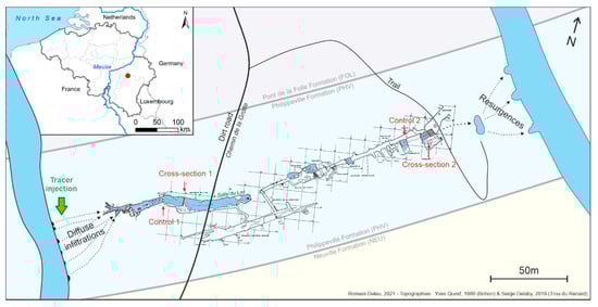
Figure 1.
The Bohon Cave system is an underground “shortcut” for a portion of the Ourthe river through the meander. It extends along the Frasnian limestones of the Philippeville Formation. Topography of the cave is adjusted from Quinif, 1980 and Delaby, 2019 [9,10].
A karstic river flows through the cave. It is fed by a portion of the nearby surface river Ourthe and resurfaces at the resurgences on the northeast where water reaches back to the Ourthe river, which draws a meander in the area. The cave river can then be considered as an underground “shortcut” between the two sides of the meander.
This site was selected because it offers a good variety of simple karstic river geometries. The river generally has a straight path from west to east through the conduits. However, large obstacles (boulders and smaller rocks) occur in the river at various places, generating local small-scale eddies and reverse currents that could generate heterogeneities in tracer dispersion.
2.2. Multi-Point Tracer Tests with a Transversal Configuration
To highlight any spatial variability in tracer concentration, three multi-point configurations can be considered: (i) along stream or longitudinal, placing fluorometers at regular intervals along the stream; (ii) transversal, placing fluorometers at a set of x (lateral position) and z (depth) coordinates along a transversal cross-section; and (iii) placing fluorometers all around a capacitive zone such as a lake. The tracer signals can then be compared with each other in terms of first arrival, peak, and breakthrough ending times, modal (peak) concentration, and curve shape.
For this study, a transversal configuration was selected with the goal of highlighting any lateral and vertical heterogeneity through a cross-section of a karstic river. Two tracer tests were performed in the Bohon Cave on 28 May 2020. Each test was performed the same day with an interval of about 3 h 30, and with the same amount of dye (20 g) injected at the same location. For both tests, a different cross-section of the river was equipped with 6 fluorometers, FluoGreen (Traqua, Namur, Belgium–www.traqua.be, accessed 20 June 2021) [1]. Cross-section 1 was located in the far-end room “Salle du Lac” in the cave, at about 90 m from the injection point (Figure 1). Cross-section 2 was located at the entrance of the cave, about 260 m from the injection point. The spatial arrangement of fluorometers was established by spacing them at a consistent interval so that the whole section could be covered. It can be visualized in Figures 4b and 5b, where 6 fluorometers are spread across the sections. For each test, a control fluorometer was placed 10–15 m upstream to assess the upstream breakthrough curve and was used for the CFD simulation.
The injection of tracers was performed at the surface, at the right bank of the Ourthe river where a portion of the water is visually lost through the ground. The use of a tube for the injection guarantees that all the tracers reach the karstic system and no tracer continues its course in the surface of Ourthe river. The selected tracer was 20 g of uranine (fluorescein).
The water level and water flow in the cave river were measured by the use of water level probes. Pressiometric probes CTD-Diver and Baro (Schlumberger, Houston, USA—www.slb.com, accessed 20 June 2021) were used to measure water and atmospheric pressures, respectively. The atmospheric pressure was subtracted from the water pressure to estimate the water level at the position of the Diver probe in the river. Multiple gauges of water flow were performed using the electromagnetic current meter Flo-Mate 2000 (Marsh McBirney—Hach, Loveland, USA—www.hach.com, accessed 20 June 2021), allowing the elaboration of a rating curve, to convert the measured water level to water flow. This allowed a good estimation of water level and water flow during the tracer tests with the goal of checking for consistency of the waterflow during both tracer tests. The flowrate was constant (0.247 m3/s) throughout the day, according to the probes data.
2.3. Calibration of Fluorometers
Tracer test data consisted of 1 min interval raw light intensity measurements at the emission wavelength of uranine [1]. This measurement was performed while a blue LED light was on, allowing for the excitation of uranine molecules. A correction of stray light was performed (as described by Poulain et al., 2017 [1]) before applying the calibration curve values to each dataset. This allowed us to obtain the final uranine concentration value at each interval for each fluorometers. Internal clocks allowed for the synchronization of each fluorometer and with the injection time.
Fluorometers were precisely calibrated in the lab before and after the test by the elaboration of a calibration curve. The curve links the raw light intensity measurement of the device with the uranine concentration. This allows the converting of raw fluorescence data to concentration in ppb. The calibration process was performed by the combination of manual and automatic calibrations (Figure 2). Manual calibration was performed by exposing the fluorometer to a bath of a precise concentration, while automatic calibration was performed by exposing the fluorometer to a bath of slowly increasing concentration using a precisely calibrated pump. The combination of both processes allowed the deletion of the pump error while still obtaining a high number of points on the calibration curve. The coefficient of determination R2 of the 2nd-order polynomial regression curve of the automatic calibration data usually reached more than 0.9999 with up to 600 points. This guaranteed the good quality of the calibration process, thus allowing for an efficient comparison of the data obtained for each fluorometer during the tracer tests.
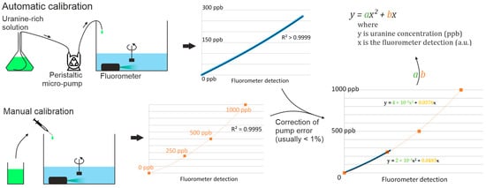
Figure 2.
Automatic and manual calibrations of the fluorometers.
2.4. Computational Fluid Dynamics (CFD) Modeling
CFD modeling was used to simulate the flow of one or more fluids through a user-drawn geometry. Hundreds of model types exist and the choice depends on the objectives. Here, the objectives were to simulate the dispersion of tracers through a karst geometry. Compared to cross-section 1, cross-section 2 has a much more complex geometry and a more turbulent flow type, with variations in the free surface level, leading to a difficult or impossible simulation. Therefore, only the cross-section 1 was computed in OpenFOAM software [11]. Model settings and boundaries were largely inspired by various hydrology papers and books with very similar objectives and model types [12,13,14,15,16,17].
2.4.1. Discretization of Karst Conduit
The computation of fluid flow was performed in a restricted geometry, which was drawn based on the site karst geometry. Four types of boundaries were considered while drawing the geometry using Blender software: an inlet, an outlet, the channel, and the water level (Figure 3).
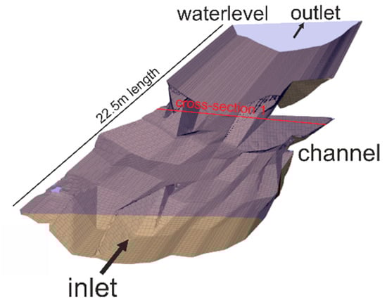
Figure 3.
Geometry and boundaries used to simulate tracer dispersion.
The inlet was drawn as a transversal cross-section at the position of the control fluorometer about 10 m upstream of cross-section 1, while the outlet was drawn the same way about 12 m downstream of the cross-section. The channel was drawn based on manual measurements of the bathymetry at regularly spaced transversal cross-sections. The water level was fixed as a reference point and can be checked for consistency with the help of the pressure probes installed on-site. The free-surface evolution was not considered here; hence, the free-surface was considered as a fixed boundary of the computational domain. Each of the four boundaries was assigned a specific patch type and boundary conditions. The whole geometry was then exported from Blender in stl file format and implemented in OpenFOAM case format using the snappyHexMesh tool. The tool was designed to generate a mesh file from Blender geometries by the use of an open-source add-on for Blender [18]. The generated mesh can directly be used to compute the flow and related variables.
2.4.2. CFD Model Type and Settings
For this study, a 3D incompressible single-phase flow model type was considered. The pisoFoam solver of the open-source OpenFOAM software is an ideal candidate and is described as a 3D transient finite volume model for incompressible single-phase flow [11]. Both pressure and velocity fields were computed by solving the Navier–Stokes equations using the PISO (Pressure Implicit with Splitting of Operators) algorithm. Additional scalar fields can be added, e.g., to compute the dispersion of a tracer through the mesh. Advection, dispersion, and molecular diffusion were computed, while sorption, desorption, and degradation were not. The molecular diffusion of uranine was set as 4.2 × 10 −10 m2/s [19].
Boundary conditions were set as follows (Table 1):

Table 1.
Boundary conditions for fields U, p, and s.
The inlet boundary was set to have a fixed velocity based on the measured flowrate the day of the tracer injection (Q = 0.247 m3/h). Flowrate was automatically converted to velocity by dividing by the surface area of the inlet geometry, and it was the only surface allowing for positive velocity. The inlet was also the only surface through which the uranine scalar could enter by an increase in scalar value at the boundary. This was performed by setting the scalar value for each time step from a table file. The table was elaborated by using the real-time tracer concentration data from the control fluorometer. Values were written in mg/L instead of ppb to keep values in the accepted range of 0 to 1. The pressure at the inlet was set as a zero gradient value extrapolated from the neighboring cells.
The outlet boundary had its pressure fixed at 0 m2/s2, allowing for the computed velocity to gain negative value (outward flow). Positive velocity was forbidden by setting an “inletOutlet” velocity condition on the outlet, to prevent any return flow and avoid instability. Uranine was set as an “inletOutlet” condition as well, allowing for a negative or null gradient and forbidding a positive gradient, preventing any tracer entrance through the outlet.
Channel and water level (symmetry) boundaries were both set as a zero-gradient condition for both pressure and uranine, preventing any flow through them. The velocity was set as a no-slip condition for the channel, which implies the computation of a wall function at the boundary, simulating friction and setting the tangential and normal velocities to 0 m/s. The water level was set as a symmetry boundary, which implies that for the tangential velocity to be computed with no wall function, no friction was considered.
2.4.3. Running and Results Extraction
The running of pisoFoam solver generated field data for each timestep across the whole mesh. Velocity U, pressure p, and scalar s were written to a hard drive at a fixed “writing” interval. Data can be visualized in 3D using the ParaView software (Video S1). Three-dimensional visualization is useful to visualize the dispersion of the tracer cloud through the geometry. In Paraview, cell data can also be extracted by selecting cells that intersect with a plane. This is useful to extract velocity and uranine data at the cross-section.
To compare tracer breakthrough curves from the on-site tracer test and CFD simulation, field data from specific cells were extracted in a csv file using the “probe” tool. Probes were located at the coordinates of the on-site cross-section fluorometers. The csv files could then be used to graph the simulated breakthrough curves for each fluorometer and compare it with on-site tracer test data.
3. Results
3.1. On-Site Tracer Tests
The multi-point dye tracing experiment in the Bohon Cave was performed on 28th May 2020 with a transversal configuration. Each fluorometer was placed at a specific set of coordinates x and z, as described earlier, and the uranine concentration was measured during a tracing experiment. The resulting concentration graphs over time (breakthrough curves) are shown in Figure 4a and Figure 5a. Table 2 synthesizes the resulting parameters.
Table 2.
First arrival, peak time, peak tracer concentration, and recovery rate for each fluorometer of cross-sections 1 and 2. Outliers or discussed values are in bold.
For cross-section 1 (90 m downstream of the injection point), the breakthrough curves of the upstream control fluorometer 1 and the six fluorometers installed along the stream cross-section 1 are shown in Figure 4a. The results show strong variabilities in peak time, peak concentration, and curve shape. The time of first arrival is consistent for each fluorometer with a first tracer signal 12 min after the injection, indicating a first arrival between 11 and 12 min. The peak time varies from 16 to 19 min (Table 2). The peak concentration has a value between 68 and 104 ppb, which represents a variability of up to 35%. End of breakthrough consistently occurs after about 50 min, where the measured light intensity reaches back to its background value corresponding to a uranine concentration of 0 ppb. The curve shape is variable. Fluorometers 8, 11, 12, and 13 show consistent values in terms of first arrival, peak time, and concentration, as well as a similar curve shape. Their peak concentration is around 90–100 ppb, reached after 16 min. Fluorometers 14 and 15 show different values for peak time and concentration and a different curve shape. Their peak concentration is around 70 ppb, reached after 19 min. This represents a difference of around 20–35% in terms of peak concentration with the previous group of fluorometers. The curve shape shows a slower concentration increase on both fluorometers 14 and 15, and a higher tailing effect on number 15. Fluorometers 14 and 15 show a strongly oscillating concentration on their tail. The tracer mass recovery rate, calculated by integrating concentration values over time and multiplying by the measured flowrate (0.289 m3/s during the injection), shows values around 79%, except for fluorometer 14, which shows a value of 66%.
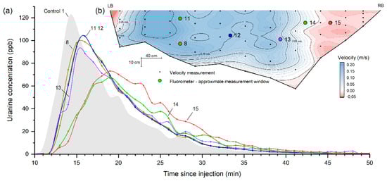
Figure 4.
(a) Breakthrough curves for each fluorometer of cross-section 1. Control fluorometer is placed 10–15 m upstream of the section (Figure 1). (b) Velocity profile of cross-section 1 and location of the fluorometers (LB: left riverbank; RB: right riverbank).
For cross-section 2 (260 m downstream of the injection), the breakthrough curves of the upstream control fluorometer 2 and the six fluorometers installed along the stream cross-section 2 are shown in Figure 5a. The results show some variabilities in peak time, peak concentration, and curve shape. The time of first arrival is consistent for each fluorometer with a first tracer signal 32 min after the injection, indicating a first arrival between 31 and 32 min. The peak time varies from 44 to 46 min. Peak concentration has a value between 49 and 55 ppb, which represents a variability of up to 11%. End of breakthrough consistently occurs after about 80 min. The curve shape is similar for each fluorometer. The tracer mass recovery rate shows values around 79%, except for fluorometer 8, showing a value of 71%. The spatial distribution of uranine seems more homogeneous in cross-section 2.
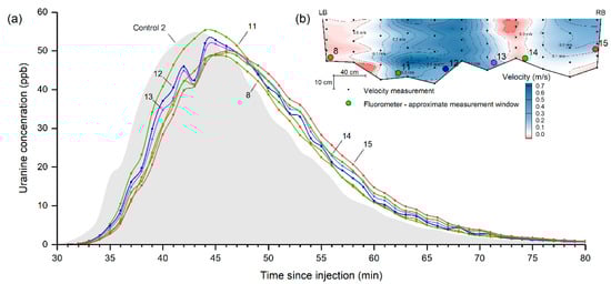
Figure 5.
(a) Breakthrough curves for each fluorometer of cross-section 2. Control fluorometer is placed 10–15 m upstream of the section (Figure 1). (b) Velocity profile of cross-section 2 and location of the fluorometers (LB: left riverbank; RB: right riverbank).
3.2. CFD Simulation
The CFD model is configured to simulate the dispersion of the tracer through the mesh. A snapshot of the tracer cloud is displayed in Figure 6b (16 min after the injection) as a visual illustration. As the simulation runs, tracking of the tracer concentration at single cells located at the position of fluorometers in cross-section 1 was performed, allowing for the drawing of breakthrough curves. These curves can then be compared with on-site results described above. The curves are displayed in Figure 6a.
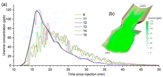
Figure 6.
(a) Simulated breakthrough curves for each fluorometer of cross-section 1; (b) 3D snapshot of tracer dispersion through the mesh at t = +950 s.
Seven simulated curves are shown in Figure 6a for cross-section 1. The results show strong variabilities in peak time and concentration and in curve shape. Fluorometers 8, 11, 12, and 13 show very similar curves, which are almost overlapped. First arrival is consistent with 11–12 min for every curve. Peak concentration is reached 16 min after the injection with a value of 118 ppb for fluorometers 8, 11, 12, and 13. For fluorometers 14 and 15, it is more difficult to find the peak as the signal is strongly oscillating. However, a 30 min moving average treatment (Figure 7) indicates a peak at t = 20 min and peak concentrations of 67 and 69 ppb for fluorometers 14 and 15, respectively. The concentration increase is much slower for fluorometers 14 and 15 (10 ppb/min vs. 45 ppb/min for 8, 11, 12, and 13) and a stronger tailing effect is observed as well.
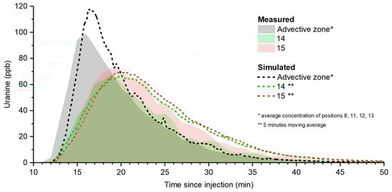
Figure 7.
CFD vs. on-site breakthrough curves at cross-section 1.
These results seem mostly consistent with on-site tracer test results. A visual comparison is proposed in Figure 7, displaying averaged breakthrough curves of fluorometers 8, 11, 12, and 13 (called advective zone, see discussion) and of fluorometers 14 and 15 (called Eddy, see discussion), for both on-site and CFD results. Some mismatches can be highlighted between the simulated and real-life data. The simulated first arrival time seems a bit late for the advective zone group (fluorometers 8, 11, 12, and 13). The simulated peak concentration is too high (118 ppb vs. 100 ppb) for the advective zone group as well. The tails of both curves 14 and 15 show higher values than on-site results, as the decrease rate is slightly lower. Simulated peak concentrations of curves 14 and 15 are consistent with on-site results, with a slightly late peak time, as the concentration increase is slightly lower than real-life data.
Globally, the simulated curve shape is very similar to the observed ones for both groups (advective and Eddy), with a slower concentration increase for 14 and 15 and a higher tailing effect. The matching of the simulation with real-life data is considered satisfying. Even though it is possible that slight changes in the mesh geometry could induce significant variations in results, multiple attempts of simulation in varied geometries showed fairly similar results; this would deserve its own focused study in the future. The distinction between advective and Eddy groups (observable in every attempt) indicates a successful simulation of hydrodynamical phenomena responsible for such variations. Therefore, this specific CFD model is considered reliable for discussing the impact of hydrodynamics on tracer test results at this site.
4. Discussion
The results indicate relatively strong variabilities in peak time, peak concentration, and curve shape. These variations could not be due to an insufficient lateral dispersion of tracers after the injection point, as the distance is assumed to be large enough (~90 m) and the local injection point configuration (diffuse water loss through collapsed debris of rock on the riverside) is assumed to guarantee a sufficient level of homogenization of tracers before the monitored cross-section. No “clean” water input is present near the cross-section and local observations strongly suggest that all infiltrated water flows into the karstic river, suggesting that all the tracers should be recovered. However, the lack of about 20% of tracers, as observed by recovery rates, might suggest the occurrence of a secondary smaller scale conduit, parallel to the Bohon Cave.
4.1. Flow Type and Implications
The measured velocities indicate a turbulent flow for both cross-sections based on the Reynolds number:
where U is the mean velocity and can be estimated by dividing the flowrate by the cross-sectional surface area; dh is the hydraulic diameter, which can be estimated as four times the ratio of cross-sectional area over its perimeter [20]; and µ is the kinematic viscosity of water set as 1.3 × 10⁻⁶ m2/s. Equation (1) can be simplified as:
where Q is the flowrate measured as 0.247 m3/s the day of the injections; and P is the cross-sectional perimeter, which is calculated using the bathymetric data for both cross-sections 1 and 2. Reynolds numbers are estimated as 66,600 and 99,000 for cross-sections 1 and 2, respectively.
Measured velocities also indicate a subcritical flow for both cross-sections based on the Froude number:
where U is the mean velocity; g is the gravitational acceleration 9.81 m2/s; and hm is the hydraulic mean depth, which can be estimated as the ratio of the cross-sectional area over the width of the cross-sectional open surface [21]. Equation (3) can be simplified as:
where l is the width of the cross-sectional open surface in m. Froude numbers are estimated as 0.035 and 0.095 for cross-sections 1 and 2, respectively.
Reynolds and Froude numbers for both cross-sections indicate a turbulent subcritical flow (Table 3); the turbulence is not at saturation and the flow can be considered moderately turbulent. This is coherent with field observations, where a slightly agitated current was observed at both sections. Turbulence suggests the importance of mechanical dispersion as a key factor for lateral dispersion of the tracer. This small-scale dispersion, combined with molecular diffusion, should allow for tracers to effectively disperse through the lower-velocity area. It should also contribute to the complete lateral dispersion of tracers in the absence of large obstacles. However, a subcritical flow induces obstacles to influence flow direction and velocity upstream. Therefore, it is possible that downstream obstacles can generate variations in local hydrodynamics at the cross-section. Such variations can be changes in velocity, changes in flow direction, increases in turbulence intensity, and the generation of eddies [22,23]. This suggests the importance of upstream and downstream river geometry on the hydrodynamics, as perturbations can travel in both directions. As solute transport is inherently controlled by the flow, changes and perturbations in local hydrodynamics could induce observable lateral and vertical heterogeneities in tracer concentration across a section. Therefore, heterogeneities in tracer tests results may suggest variations in local hydrodynamics.
Table 3.
Hydraulic parameters of both cross-sections 1 and 2. A = cross-sectional area; P = cross-sectional perimeter; l = river surface width at the cross-section; U = mean velocity calculated by dividing the measured flowrate by the cross-sectional area; Re = Reynolds number; F = Froude Number.
4.2. Cross-Section 1 and CFD Simulation
Observed heterogeneities in cross-section 1 include a slower concentration increase, inducing delays in peak, lower peak concentration, higher tailing effects, and lower recovery rate. These variations are mostly observed in cross-section 1 at positions 14 and 15. Simulated concentrations at specific timesteps show consistent results with a lateral and vertical difference of concentration reaching more than 80% at some time, and which can be visualized in Figure 8 where the impact of the eddy is clearly visible on the right side. These variations can be correlated with the velocity profile, where lower or negative velocities are observed and can be associated with a delayed and lower peak in uranine concentration. Lower or negative velocity can be due to friction between water and the materials on the riverbed and sides, or due to local recirculations, in the vertical or horizontal plane. Obstacles upstream or downstream of the section can also induce lower speed for a subcritical flow. The large-negative-velocity area on the right side of cross-section 1 (Figure 4b) can be associated with the presence of a 2 m-wide rock 0.5 m downstream of the cross-section. This obstacle generates the presence of a local eddy current (Figure 10a), explaining the negative velocity and suggesting that such a perturbation in local hydrodynamics can have great impact on breakthrough curves for fluorometers placed in the area of impact of such obstacles. This impact seems at least significant for such a short-timed tracer breakthrough (i.e., less than an hour). The delay in the peak can be explained by a larger amount of time required for the tracer to reach the inner part of the eddy current, while the higher tail concentrations for fluorometer 15 indicate the tendency for the tracer to remain longer in the Eddy current. A lower recovery value of 66% for fluorometer 14 might indicate that some low-velocity areas receive less tracers than more advective zones do. In low-velocity areas, closer to the obstacle, advection is much lower and contributes less to the transport of tracers. Dispersion can then become the major source of solute transport, thanks to turbulence, while molecular diffusion must probably remain negligible. This allows for a breakthrough curve to still occur at these near-zero velocity areas, but it can greatly slow down the concentration increase and decrease as well, at least at this timescale. Peak concentration can then be much lower than in more advective zones.
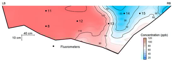
Figure 8.
Simulated concentration at t = +16 min across section 1.
The CFD simulation at cross-section 1 also indicates a delay and lower peak for fluorometers 14 and 15. This delay induces strong lateral and vertical variations in concentration across the section, as seen in Figure 8, where the right side of the section shows more than 80% less tracer concentration at some specific time. Simulated streamlines (Figure 9) indicate the presence of a large eddy at positions 14 and 15, which is coherent with field observations and tracer tests results. The CFD simulation allows for a visual observation of flow and tracer cloud dispersion in 3D at the location of the cross-section. This visualization supports field data and helps provide insights into the hydrodynamical phenomena responsible for heterogeneities in tracer dispersion. This implies the observations of correlations between the velocity profile and tracer dispersion, but also the influence of the river geometry over the hydrodynamics, and thus the tracer test results.
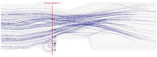
Figure 9.
Simulated streamlines at cross-section 1 (flow is from left to right). The eddy circulation is clearly visible on the right side of the stream.
4.3. Cross-Section 2
In cross-section 2, only some minor variabilities of breakthrough curves are observed (Figure 5a). Fluorometer 8 shows slightly lower peak concentrations and recovery rates (71%), which is coherent with the presence of a low-velocity zone on the left bank downstream of a large rock (Figure 10b). Fluorometer 8 is placed inside an isolated portion of the river, where advection seems limited. The presence of an eddy current can be hypothesized. However, no significant delay in peak is observed, as it was in similar situation in section 1, and field observations show that no eddy circulation of the scale observed on section 1 is possible there, due to the smaller dimension of this restricted zone. Observed negative velocities are of a much lower scale than in the eddy of section 1. Field observations also indicate the frequent occurrence of small “jets” of water from the nearby advective stream into this restricted zone, which could regularly bring tracers there. This would allow for the position 8 fluorometer to show a similar breakthrough curve than the fluorometers in the advective stream, and it can be correlated with the high Reynolds number (Table 3) linked to the turbulent nature of the flow there.
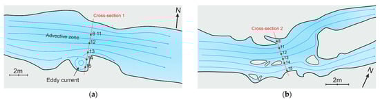
Figure 10.
Synthetic representation of streamlines and fluorometer locations for cross-sections 1 (a) and 2 (b).
A few meters upstream of the section, a hydrodynamic separation is observed, and two main advective streams appear on each side of a set of large rocks in the middle of the stream (Figure 10b). This allows for the occurrence of a low-negative-velocity area between positions 13 and 14. Eventually, this stream split continues downstream with a clear separation of the stream in two separate conduits. Field observations indicate that the upstream split is concordant with the downstream one, and that only limited mixing occurs between the two advective streams at and downstream of the section. It should also be noted that the left stream shows higher velocities and dimensions as well. This is coherent with the slightly delayed peak for position 14 and 15, along the secondary right-sided stream. The lower velocity of the right stream induces a slight delay of the tracers to the cross-section.
4.4. Implications and Perspectives
As discussed, the results of this study of short-timescale tracer breakthroughs (i.e., less than an hour) show significant heterogeneities in tracer concentration in space and time. These heterogeneities are directly correlated with hydrodynamical phenomena (eddy, slow zone, dead zone, turbulence, and stream separation), and can thus have a significant impact on the dispersion of tracers on a higher scale. The impact of various hydrodynamic phenomena over the dispersion of tracers (and thus solute transport) has been largely studied by various authors in a quantitative way and by fluid flow simulation as well [2,3,4,5,6,7,24,25]. These studies highlight the tailing effect on breakthrough curves downstream of various hydrodynamic anomalies such as the ones observed in this study. Slow or dead zones allow for a portion of tracers to be “stored” and released after the peak time, hence inducing tailing effects that can accumulate over a large scale [2,3]. This storing and late release is clearly observable on the small-scale heterogeneities observed in the Bohon Cave, and especially in cross-section 1. These internal observations of the impact of eddies and slow or dead zones could potentially lead to more insight into the large-scale impact of such features, and a more advanced quantification of the impact on the longitudinal dispersion of a tracer cloud over large distances.
The evaluation of the significance of the fluorometer positioning on the tracer test results can be assessed as well with the use of multi-point tracer tests and CFD modeling. This significance is most probably directly correlated with the occurrence of the aforementioned hydrodynamic phenomena. Thus, a review of tracer test methodologies in general can be investigated by performing more multi-point dye tracing manipulations in various karst geometries with the scope of highlighting and explaining any heterogeneity in tracer dispersion and discussing its impact on large-scale tracer dispersion. In the scope of this study, it seems apparent that placing the fluorometer in the main advective stream is necessary to ensure that hydrodynamic phenomena are not influencing the breakthrough curve shape. This is probably especially valuable at short timescales and for complex geometries with obstacles, side pools, eddies, etc.
Heterogeneities in tracer dispersion and discussing its impact on large-scale tracer dispersions are even more applicable for the question of solute transport and, particularly, the vulnerability of a karstic environment to pollutants in general. As the question of karst vulnerability has been largely studied [26,27,28,29], quantification of the solute storage in eddies and slow or dead zones by multi-point tracer tests could lead to the rigorous assessment of their implications to the large-scale dispersion of pollutants in karstic environments.
5. Conclusions
Transversal multi-point tracer tests performed in Bohon Cave (Belgium) in May 2020 provided insight into the lateral and vertical heterogeneities in tracer distribution and breakthrough curve shapes across a karstic river section. Results of the short-timescale (i.e., less than an hour) tracer breakthrough curves from the two cross-sections in the cave showed significant variations in terms of curve shape, peak delay, peak concentration, and recovery rates. These variations can be well correlated with the velocity profile of the cross-section. In this study, three hydrodynamical phenomena were highlighted by tracer test results and by CFD simulations of one of the cross-sections. Quantification of the impact of those hydrodynamical “anomalies” over the tracer tests results can be assessed by field data. This can also be performed in complementarity with CFD simulation, which allows one to complete the field observations by providing more insight into the velocity distribution in the monitored area and by computing simulated breakthrough curves that can be correlated with field data. In general, the 3D observation of the dispersion of the tracer cloud through the mesh by CFD simulation is of great help for the interpretation of field tracer test data.
An eddy current induces negative velocity on one side of cross-section 1 and is due to the presence of a small side pool upstream of a large obstacle. This eddy is associated with a significant delay and lower concentration of the breakthrough peak, and a lower recovery rate. At a specific time, differences of up to 57% in tracer concentration are observed between the eddy and the advective stream at the center of the river. This is due to a lower contribution of advection to the tracer transport, as the circulating velocity is much lower than in the center of the river. Dispersion through turbulences then becomes a key factor for the tracer transport inside the eddy, in combination with the circulating advective eddy current and the turbulent dispersion of the solute. This eddy is well simulated by the CFD model, and simulated breakthrough curves are well correlated with the observed ones. This indicates that the eddy is in fact responsible for the lateral variations in tracer distribution in cross-section 1. In cross-section 2, a “dead” zone has been monitored but shows similar curves to nearby advective streams, thanks to the frequent occurrence of small “jets” of water into the dead zone, allowing for the tracers to reach inside, in combination with molecular diffusion. A split of the stream also occurs in section 2, inducing a slight delay of the peak in the secondary stream on the right side of section 2.
Those observations indicate that the river geometry and obstacles can have significant impact on tracer test results, at least at this short timescale (i.e., less than an hour). Restricted zones with low or negative velocities can induce significantly different results than main advective streams in a river. This is especially valuable in karstic environments where large rocks and boulders are often present in the river, or where the river flows through complex geometries with many divergences, convergences, dead zones, etc. Tracer tests user should remain aware of this and attempt to place their monitoring device in the advective stream when possible. Many other types of geometries and obstacles exist in nature. Studies of the quantification of the spatial and temporal heterogeneities of tracer distribution can be attempted to (i) assess the impact of the placement of fluorometers on tracer tests results and to give recommendations on an efficient placement; and to (ii) obtain more insight into the large-scale impact of hydrodynamical features (e.g., eddy, slow zone, dead zone, stream split, and turbulence), and a more advanced quantification of their cumulative effect on the longitudinal dispersion of a tracer cloud (and thus, solute transport and pollutant) over large distances.
Supplementary Materials
The following are available online at https://www.mdpi.com/article/10.3390/hydrology8040168/s1, Video S1: CFD simulation of the tracer cloud dispersion through the mesh. The concentration (s) is in mg/L.
Author Contributions
Conceptualization, R.D., A.P. and V.H.; methodology, R.D., G.R. and V.H.; software, R.D. and S.S.F.; validation, R.D.; formal analysis, R.D.; investigation, R.D. and V.H.; resources, R.D., S.S.F. and A.P.; data curation, R.D.; writing—original draft preparation, R.D.; writing—review and editing, R.D., S.S.F., A.P. and V.H.; visualization, R.D.; supervision, V.H.; project administration, V.H. All authors have read and agreed to the published version of the manuscript.
Funding
This research received no external funding.
Data Availability Statement
Data are contained within the article or supplementary material.
Acknowledgments
We would like to acknowledge the Department of Nature and Forests (DNF) of the public service of Wallonia (SPW) and Charles Bernard for the authorization and provision of access to the Bohon Cave.
Conflicts of Interest
The authors declare no conflict of interest.
References
- Poulain, A.; Rochez, G.; Van Roy, J.-P.; Dewaide, L.; Hallet, V.; De Sadelaer, G. A Compact Field Fluorometer and Its Application to Dye Tracing in Karst Environments. Hydrogeol. J. 2017, 25, 1517–1524. [Google Scholar] [CrossRef] [Green Version]
- Hauns, M.; Jeannin, P.-Y.; Atteia, O. Dispersion, Retardation and Scale Effect in Tracer Breakthrough Curves in Karst Conduits. J. Hydrol. 2001, 241, 177–193. [Google Scholar] [CrossRef]
- Hauns, M.; Jeannin, P.-Y.; Hermann, F. Tracer Transport in Karst Underground Rivers: Tailing Effect from Channel Geometry. Bull. D’hydrogéologie 1998, 16, 123–142. [Google Scholar]
- Morales, T.; Uriarte, J.A.; Olazar, M.; Antigüedad, I.; Angulo, B. Solute Transport Modelling in Karst Conduits with Slow Zones during Different Hydrologic Conditions. J. Hydrol. 2010, 390, 182–189. [Google Scholar] [CrossRef]
- Hauns, M. Modeling Tracer and Particle Transport under Turbulent Flow Conditions in Karst Conduit Structures. Ph.D. Thesis, University of Neuchâtel, Neuchâtel, Switzerland, 2000. [Google Scholar]
- Perrin, J.; Luetscher, M. Inference of the Structure of Karst Conduits Using Quantitative Tracer Tests and Geological Information: Example of the Swiss Jura. Hydrogeol. J. 2008, 16, 951–967. [Google Scholar] [CrossRef]
- Zagouras, N. Etude de La Dispersion de Traceurs Fluorescents En Conduits Karstiques; University of Brussels: Brussels, Belgium, 2019. [Google Scholar]
- Barchy, L.; Marion, J.M. Geological Map of Wallonia, Durbuy-Mormont N°55/1-2 and Its Leaflet. SPW/Ed. Cart. In press. Available online: http://geologie.wallonie.be (accessed on 13 August 2021).
- Quinif, Y. Etude Karstologique de La Grotte de Bohon. Rev. Belge Geogr. 1980, 104, 47–62. [Google Scholar]
- Delaby, S. Topographie Provisoire Du Trou Du Renard. 2019. [Google Scholar]
- Greenshields, C.J.; CFD Direct Ltd. The OpenFOAM Foundation OpenFOAM: User Guide V9; OpenFOAM Foundation Ltd.: London, UK, 2021; p. 241. Available online: https://cfd.direct/openfoam/user-guide (accessed on 20 June 2021).
- Alvarez, L.V.; Schmeeckle, M.W.; Grams, P.E. A Detached Eddy Simulation Model for the Study of Lateral Separation Zones along a Large Canyon-bound River. J. Geophys. Res. Earth Surf. 2017, 122, 25–49. [Google Scholar] [CrossRef]
- Bates, P.D.; Lane, S.N.; Ferguson, R.I. Computational Fluid Dynamics: Applications in Environmental Hydraulics; Bates, P.D., Lane, S.N., Ferguson, R.I., Eds.; John Wiley & Sons, Ltd.: Chichester, UK, 2005; Volume 4, ISBN 9780470015193. [Google Scholar]
- Farhadi, A.; Mayrhofer, A.; Tritthart, M.; Glas, M.; Habersack, H. Accuracy and Comparison of Standard K-ϵ with Two Variants of k-ω Turbulence Models in Fluvial Applications. Eng. Appl. Comput. Fluid Mech. 2018, 12, 216–235. [Google Scholar] [CrossRef] [Green Version]
- Herrera-granados, O. Computational Fluid Dynamics (CFD) in River Engineering: A General Overview. In Proceedings of the II International Interdisciplinary Technical Conference of Young Scientists, Poznań, Poland, 20–22 May 2009. [Google Scholar]
- Lindblad, D. Implementation and Run-Time Mesh Refinement for the k—Omega SST DES Turbulence Model When Applied to Airfoils; Reports of the 2013 CFD OpenSource Software PhD Course; Chalmers Tekniska Högskola: Göteborg, Sweden, 2013; p. 65. Available online: http://www.tfd.chalmers.se/~hani/kurser/OS_CFD_2013/DanielLindblad/k-Omega-SST-DES-Report.pdf (accessed on 22 July 2021).
- Rodi, W. Turbulence Modeling and Simulation in Hydraulics: A Historical Review. J. Hydraul. Eng. 2017, 143, 03117001. [Google Scholar] [CrossRef]
- Keskitalo, T. SnappyHexMesh GUI Addon for Blender. Github Repository. 2020. Available online: https://github.com/tkeskita/snappyhexmesh_gui (accessed on 7 September 2020).
- Casalini, T.; Salvalaglio, M.; Perale, G.; Masi, M.; Cavallotti, C. Diffusion and Aggregation of Sodium Fluorescein in Aqueous Solutions. J. Phys. Chem. B 2011, 115, 12896–12904. [Google Scholar] [CrossRef] [PubMed] [Green Version]
- Koch, P. Equivalent Diameters of Rectangular and Oval Ducts. Build. Serv. Eng. Res. Technol. 2008, 29, 341–347. [Google Scholar] [CrossRef]
- United States Bureau of Reclamation. Water Measurement Manual, 3rd Edition Revised Reprinted; United States Bureau of Reclamation: Washington, DC, USA, 2001; ISBN 9780160925108.
- Chow, V.T. Open-Channel Hydraulics; McGraw-Hill: New York, NY, USA, 1959. [Google Scholar]
- Tritton, D.J. Physical Fluid Dynamics; Van Nostrand Reinhold Company: New York, NY, USA, 1977; ISBN 9788420548470. [Google Scholar]
- Gooseff, M.N.; Bencala, K.E.; Wondzell, S.M. Solute transport along stream and river networks. In River Confluences, Tributaries and the Fluvial Network; Rice, S.P., Roy, A.G., Rhoads, B.L., Eds.; John Wiley & Sons, Ltd.: Hoboken, NJ, USA, 2008; pp. 395–417. [Google Scholar]
- Gooseff, M.N.; LaNier, J.; Haggerty, R.; Kokkeler, K. Determining In-Channel (Dead Zone) Transient Storage by Comparing Solute Transport in a Bedrock Channel-Alluvial Channel Sequence, Oregon. Water Resour. Res. 2005, 41. [Google Scholar] [CrossRef] [Green Version]
- Bencala, K.E.; Walters, R.A. Simulation of Solute Transport in a Mountain Pool-and-Riffle Stream: A Transient Storage Model. Water Resour. Res. 1983, 19, 718–724. [Google Scholar] [CrossRef]
- Morales, T.; Fdez. de Valderrama, I.; Uriarte, J.A.; Antigüedad, I.; Olazar, M. Predicting Travel Times and Transport Characterization in Karst Conduits by Analyzing Tracer-Breakthrough Curves. J. Hydrol. 2007, 334, 183–198. [Google Scholar] [CrossRef]
- Ronayne, M.J. Influence of Conduit Network Geometry on Solute Transport in Karst Aquifers with a Permeable Matrix. Adv. Water Resour. 2013, 56, 27–34. [Google Scholar] [CrossRef]
- Field, M.S.; Pinsky, P.F. A Two-Region Nonequilibrium Model for Solute Transport in Solution Conduits in Karstic Aquifers. J. Contam. Hydrol. 2000, 44, 329–351. [Google Scholar] [CrossRef]
Publisher’s Note: MDPI stays neutral with regard to jurisdictional claims in published maps and institutional affiliations. |
© 2021 by the authors. Licensee MDPI, Basel, Switzerland. This article is an open access article distributed under the terms and conditions of the Creative Commons Attribution (CC BY) license (https://creativecommons.org/licenses/by/4.0/).