Impact of Pumping Rate on Contaminant Transport in Groundwater—A Numerical Study

Abstract

Public supply wells are commonly considered one of the most significant sources of freshwater on Earth. Therefore, potential well water contamination can conceivably be regarded as a crucial issue that is closely correlated with both environmental protection and water demand. In the present study, a three-dimensional numerical model is developed to simulate unsteady and spatially varying groundwater flow, along with contaminant migration. Besides, the proposed model is capable of investigating well water quality by the change of the wells’ pumping rates. The developed model uses a finite-volume time splitting numerical technique to solve governing groundwater flow and soluble contaminant transport equations. Comparison of the numerical simulation results with analytical solutions, as well as experimental and field data, clearly demonstrates the satisfactory performance of the present model. The fundamental aim of the study is to evaluate the effect of pumping rate and its variations on pollution migration through saturated porous media. To meet this purpose, contaminant concentrations and contaminants’ travel time were studied under different pump flow rate conditions. The modeling results revealed that choosing an optimum range for the pumping rate increases contaminant travel time and reduces aquifer vulnerability.

1. Introduction

The significance of groundwater management has increased in recent years, due to increasing population growth rates and water needs. Groundwater pumping aids in meeting the ever-increasing demand for water on a sustainable basis although both the quality and quantity of groundwater resources have degraded in recent years [1]. The growing public concern regarding pollutant emissions includes considering groundwater contamination as a crucial subject in hydrogeology; thus, there has been a dramatic interest increase in the assessment and prediction of contaminant migration in groundwater [2,3,4].

The aquifer vulnerability is directly related to the hydraulic conductivity of porous media, the depth to the water table, the groundwater recharge, pollution source, and groundwater flow conditions [5,6]. Travel time and pollutant concentration are the overriding factors for determining the vulnerability of aquifers.

In recent years, various methods have been used by researchers to investigate contaminant transport through porous media. Both analytical and numerical techniques have frequently been used to study groundwater pollution. Bessel function expansion, Green’s Function, and Eigen function expansions have been found as the most suitable analytical techniques [7,8,9]. Classical numerical methods, including finite difference, finite element, and finite volume schemes, have been the common approaches for groundwater modeling in recent years [10,11,12,13]. In several investigations, both experimental and numerical methods have been used to study contaminant transport [14]. In recent years, some novel methods have been proposed to overcome the limitations of the classical numerical methods [15,16,17,18,19].

In previous years, detection and remediation of well water contamination have posed novel challenges to groundwater resource managers. As a result, the effective management of groundwater quality has become one of the most complex problems faced by modern groundwater researchers. Halford et al. discussed improvements in pumped water quality from public supply wells in Antelope Valley (California) obtained through grouting of selected intervals to reduce the entry of arsenic-bearing water [20]. Johnson et al. examined the impact of several pumping scenarios on leakage from an unconfined aquifer to a confined aquifer and concluded that a single inactive multi-aquifer well can contribute nearly 10% of total public water supply well flow over a wide range of pumping rates [21].

Several solutions have been developed for addressing the interaction between the pumping rate and water quality of a given well, using analytical and numerical techniques. Park and Aral solved a multi-objective optimization problem using a genetic algorithm to determine pumping rates and well locations for the prevention of saltwater intrusion, while satisfying desired discharge rates in aquifers [22]. Further, Kalwij and Peralta presented a simulation/optimization model for determining optimal pumping strategies, considering the uncertainty of the aquifer’s parameters [23]. Both groundwater flow and pollution migration through long-screened wells were simulated by Zinn and Konikow [24]. Their findings indicated that intra-borehole flow had a direct impact on the groundwater flow within a conceptual aquifer system. Additionally, Sharief et al. used a coupled finite element method, which was embedded with the genetic algorithm (GA) to find an optimal pumping pattern for the remediation of aquifers [25]. They concluded that using the pump and treat method can remediate the pollution plume.

Later, the impact of seasonal changes on both the quality and age of water pumped from public supply wells was investigated by Bexfield and Jurgens [26]. They demonstrated that either abatement or cessation of pumping from public supply wells causes contaminant migration through intra-borehole flow. In another study, Cyriac and Rastogi investigated an optimal pumping policy using a coupled finite element-particle swarm simulation–optimization model [27]. Their model considered the collective drawdown of the wells to find the maximum allowable pumping discharge, along with the location of the wells to mitigate pollution. Rodriguez-Pretelin and Nowak developed a management scheme fulfilling the groundwater demand and decreasing the impact of transient flow on the abstraction zone through optimally redistributing pumping rates within well fields [28]. Finally, Dey and Prakash carried out density-dependent simulations to design a pumping management strategy in a coastal aquifer [29]. Their method determined the maximum pumping rate without seawater intrusion.

It is of great importance to accurately predict the migration path and pollution plume during different pumping rates, in the management and protection of groundwater resources. In recent studies, such as studies by Medici et al. [30] and Medici and West [31], groundwater flow and aquifer vulnerability have been studied at steady-state conditions. Steady-state flow conditions are fairly rare, and unsteady conditions can occur as a result of daily and seasonal fluctuations as well as time-dependent hydraulic stresses, such as pumping or recharge. Consequently, transient flow scenarios should be incorporated, and the influence of unsteady-state groundwater flow on contaminant fate should be considered.

The objective of this study is to investigate the effect of different pumping rates on the contaminant plume, by the proposed numerical model, which can simulate the transient groundwater flow and pollution transport through saturated porous media. The model can be used as an effective tool for predicting pollution migration and making decisions in the management of water resource systems.

2. Model Development

2.1. Governing Groundwater Flow Equation

The equation of transient groundwater flow through non-homogeneous anisotropic porous media, as presented by Darcy’s Law, is derived by combining a continuity equation with Darcy’s Law. This equation is known as the Boussinesq equation. The groundwater flow in saturated porous media is presented by the following equation [32]:

$${\mathrm{S}}_{\mathrm{s}}\frac{\partial \mathrm{h}}{\partial \mathrm{t}}=\nabla ·\left(\mathrm{K}·\nabla \mathrm{h}\right)$$

(1)

where $\mathrm{K} \left[{\mathrm{LT}}^{-1}\right]$ is the hydraulic conductivity matrix, which includes the hydraulic conductivity of the soil in different directions; $\mathrm{h} \left[\mathrm{L}\right]$ is the hydraulic head;${ \mathrm{S}}_{\mathrm{s}} \left[L^{-1}\right]$ is specific storage; and $\mathrm{t} \left[\mathrm{T}\right]$ represents time.

2.2. Governing Contaminant Transport Equation

The transport of solute in porous media, as in groundwater, can be described by three processes: advection, hydrodynamic dispersion, and physical-chemical or biochemical reactions. The transport of contaminants in flowing groundwater is derived from the principle of conservation of mass. A general form of the solute-transport equation is as follows:

$${\mathrm{R}}_{\mathrm{d}}\frac{\partial \mathrm{C}}{\partial \mathrm{t}}=\nabla ·\left(\mathrm{D}\nabla \mathrm{C}\right)-\nabla ·\left(\mathrm{V} \mathrm{C}\right)-{\mathsf{\lambda }\mathrm{R}}_{\mathrm{d}}\mathrm{C}$$

(2)

where $\mathrm{C}\left(\mathrm{x},\mathrm{y},\mathrm{z},\mathrm{t}\right)$ is the contaminant concentration $\left[{\mathrm{ML}}^{-3}\right]$; $\mathrm{D}$ is the coefficient of hydrodynamic dispersion $\left[{\mathrm{L}}^2{\mathrm{T}}^{-1}\right]$; $\mathrm{V}$ is the seepage velocity $\left[{\mathrm{LT}}^{-1}\right]$; $\mathsf{\lambda }$ is the contaminant decay rate; and ${\mathrm{R}}_{\mathrm{d}}$ is the retardation factor that is used for considering the difference between flow seepage and solute contaminant velocity, as a result of physical, biological, and chemical mechanisms. Contaminant dilution due to hydrodynamic dispersion is represented by the first term on the right side of Equation (2). The second term of the equation constitutes advective transport, describing the movement of solutes in flowing groundwater. Note that in this research, a non-reactive solute contaminant was considered to simulate pollution migration; therefore, the third term on the right side of Equation (2) was neglected. The hydrodynamic dispersion coefficients in different directions are given as

$$D_i={\alpha }_L\frac{v_i^2}{\left|V\right|}+{\alpha }_{TH}\frac{v_i^2}{\left|V\right|}+{\alpha }_{TV}\frac{v_i^2}{\left|V\right|}+D^{\ast }\hspace{1em}\hspace{1em}\hspace{1em}\hspace{1em}\hspace{1em}\left(i=1,2,3\right)$$

(3)

where $D_1$, $D_2$, and $D_3$ are hydrodynamic dispersion coefficients in three Cartesian coordinate axes. ${\alpha }_L$, ${\alpha }_{TH}$, and ${\alpha }_{TV}$ are longitudinal, horizontal transverse, and vertical transverse dispersivity, respectively.$v_1$, $v_2$, and $v_3$ are velocity vectors in the Cartesian coordinate axes. $D^{\ast }$ is the coefficient of molecular diffusion, and $\left|V\right|$ is the average velocity vector. The longitudinal dispersivity is proportional to the measurement scale. For porous media, the flow direction dispersivity is as follows [33]:

$${\alpha }_L=0.2 L^{0.44}$$

(4)

where L $\left[L\right]$ is the flow distance (path). Both transverse dispersivities are generally smaller than longitudinal, and in most cases, they are 1/10 to 1/100 of the longitudinal dispersivity [34]. In recent years, some research has been conducted to get acute insight into the relationship between longitudinal dispersivity and transverse dispersivities [35].

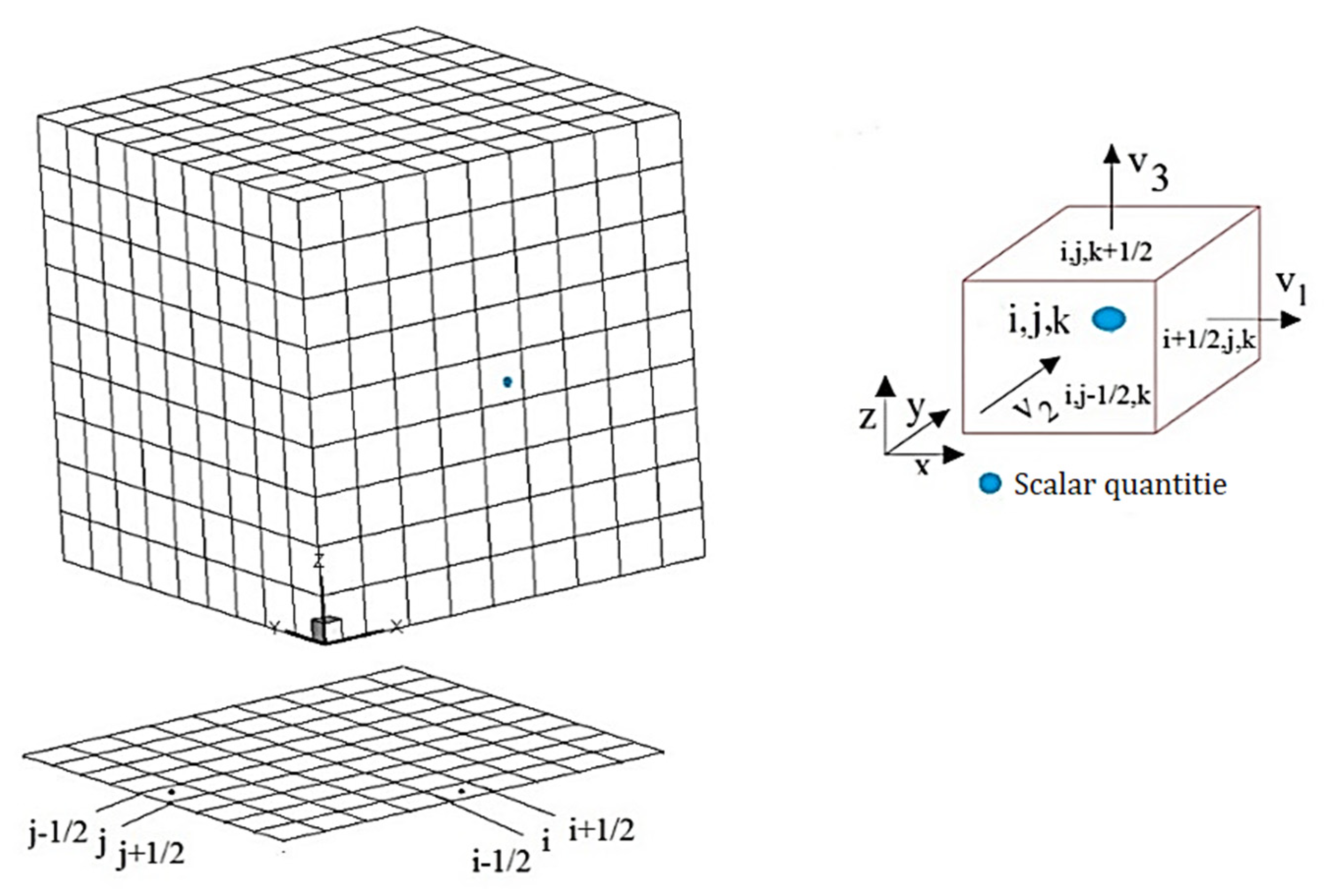
3. Numerical Solution

The proposed model uses a finite-volume time splitting method approach to solve the governing equations in porous media. The scalar quantities, such as contaminant concentration and hydraulic head, are defined at the center of the cells, while the velocity components are located at the faces, as shown in Figure 1. The flux passing through each cell face can be regarded as the most important issue in FVM.

The calculated flux for each of the cell faces is added to the mass of the downstream cell and subtracted from the upstream cell at the same time, whereby conservativity is guaranteed. The change of mass inside the cell $i$ during a specific time interval $\Delta \mathrm{t}$ can be calculated as

$${\mathrm{mass}}_{\mathrm{i}}^{\mathrm{n}+1}={\mathrm{mass}}_{\mathrm{i}}^{\mathrm{n}}+\Delta \mathrm{t} \left({(\mathrm{Flux})}_{i-1/2}-{\left(\mathrm{Flux}\right)}_{i+1/2}\right)$$

(5)

where the term on the left-hand side demonstrates the mass inside the cell $i$ at a new time step, and the first term on the right-hand side represents the mass inside the cell $i$ at the old time step.

Another technique used in the present model is the time splitting method. The key feature of this method is solving the governing equations in different steps. This method not only reduces computation cost, but also elevates the numerical model’s precision. The time splitting algorithm, proposed by Yanenko [36], has widely been employed to numerically solve the governing partial differential equations. The aforementioned methods are employed to solve both groundwater and contaminant transport equations.

3.1. Groundwater Equation

Finite volume discretization can be written for the Boussinesq equation, giving

$${ \mathrm{S}}_{\mathrm{s}}\frac{{\mathrm{h}}^{\mathrm{n}+1}-{\mathrm{h}}^{\mathrm{n}}}{\Delta \mathrm{t}}=\frac{\partial }{\partial {\mathrm{x}}_i}\left({\mathrm{K}}_{{\mathrm{x}}_i}\frac{\partial \mathrm{h}}{\partial {\mathrm{x}}_i}\right) \left(i=1,2,3\right)$$

(6)

$${\mathrm{h}}^{\mathrm{n}+1}={\mathrm{h}}^{\mathrm{n}}+\frac{\Delta \mathrm{t}}{\Delta {\mathrm{x}}_i} \left({({\mathrm{K}}_{{\mathrm{x}}_i}\frac{\partial \mathrm{h}}{\partial {\mathrm{x}}_i})}_{i-1/2}-{({\mathrm{K}}_{{\mathrm{x}}_i}\frac{\partial \mathrm{h}}{\partial {\mathrm{x}}_i})}_{i+1/2}\right) \left(i=1,2,3\right)$$

(7)

where ${({\mathrm{K}}_{{\mathrm{x}}_i}\frac{\partial \mathrm{h}}{\partial {\mathrm{x}}_i})}_{i-1/2}$ and ${({\mathrm{K}}_{{\mathrm{x}}_i}\frac{\partial \mathrm{h}}{\partial {\mathrm{x}}_i})}_{i+1/2}$ are fluxes passing from the downstream and the upstream of the cell $i$ faces, respectively. A second-order (in space) estimation for space derivation at the cell face can be written as

$${\left(\frac{\partial \mathrm{h}}{\partial {\mathrm{x}}_i}\right)}_{i-1/2}\approx \frac{1}{\Delta x_i}\left(h_i-h_{i-1}\right) \left(i=1,2,3\right)$$

(8)

In the next part, the time splitting method is used to solve the discretized groundwater equation. The solution procedure consists of one main step, which has three stages. The three stages include calculating the fluxes in three Cartesian coordinate axes. Full details about using the finite-volume time splitting method, as well as simulation of the free surface by an iterative algorithm, can be found in the study by Ahmadi [17,19].

3.2. Contaminant Transport Equation

Employing the time splitting algorithm, the contaminant transport equation can be split into two main steps. The first step, which consists of three stages, solves the advection term, and the second step solves the dispersion term in three stages. In the first step, the contaminant concentration is computed in the time step $\mathrm{n}+1/2$ by solving the advection term. The second step is to compute the contaminant concentration by solving the dispersion term in the time step $\mathrm{n}+1$.

3.2.1. Advection Term

Finite volume discretization can be written for the advection term, giving

$$\frac{\partial \mathrm{C}}{\partial \mathrm{t}}=-\frac{\partial ({\mathrm{v}}_{{\mathrm{x}}_i}\mathrm{C})}{\partial {\mathrm{x}}_i} \left(i=1,2,3\right)$$

(9)

$${\mathrm{C}}^{\mathrm{n}+1/2}={\mathrm{C}}^{\mathrm{n}}+\frac{\Delta \mathrm{t}}{\Delta {\mathrm{x}}_i} \left({({\mathrm{v}}_{{\mathrm{x}}_i}\mathrm{C})}_{i-1/2}-{({\mathrm{v}}_{{\mathrm{x}}_i}\mathrm{C})}_{i+1/2}\right) \left(i=1,2,3\right)$$

(10)

where ${({\mathrm{v}}_{{\mathrm{x}}_i}\mathrm{C})}_{i-1/2}$ and ${({\mathrm{v}}_{{\mathrm{x}}_i}\mathrm{C})}_{i+1/2}$ are fluxes passing from downstream and the upstream of the cell $i$ faces, respectively.

Employing the FVM for the advection term, flux is presented as

$$\mathrm{Flux}=\frac{1}{\Delta \mathrm{t}}{{\displaystyle \int }}_{{\mathrm{t}}^{\mathrm{n}}}^{{\mathrm{t}}^{\mathrm{n}+1/2}}{\mathrm{v}}_{{\mathrm{x}}_i}\mathrm{Cdt}\hspace{1em}\hspace{1em}\hspace{1em}\hspace{1em}\left(i=1,2,3\right)$$

(11)

This step includes three stages in all directions, and the advection terms in all the stages are solved using the Fromm scheme, as an explicit second-order upwind scheme.

3.2.2. Dispersion Term

Finite volume discretization can be written for the dispersion term, giving

$$\frac{\partial \mathrm{C}}{\partial \mathrm{t}}=\frac{\partial }{\partial {\mathrm{x}}_i} \left({\mathrm{D}}_{{\mathrm{x}}_i}\frac{\partial \mathrm{C}}{\partial {\mathrm{x}}_i}\right) \left(i=1,2,3\right)$$

(12)

$${\mathrm{C}}^{\mathrm{n}+1}={\mathrm{C}}^{\mathrm{n}+1/2}+\frac{\Delta \mathrm{t}}{\Delta {\mathrm{x}}_i} \left({({\mathrm{D}}_{{\mathrm{x}}_i}\frac{\partial \mathrm{C}}{\partial {\mathrm{x}}_i})}_{i-1/2}-{({\mathrm{D}}_{{\mathrm{x}}_i}\frac{\partial \mathrm{C}}{\partial {\mathrm{x}}_i})}_{i+1/2}\right) \left(i=1,2,3\right)$$

(13)

where ${({\mathrm{D}}_{{\mathrm{x}}_i}\frac{\partial \mathrm{C}}{\partial {\mathrm{x}}_i})}_{i-1/2}$ and ${({\mathrm{D}}_{{\mathrm{x}}_i}\frac{\partial \mathrm{C}}{\partial {\mathrm{x}}_i})}_{i+1/2}$ are the upstream and downstream fluxes of the cell $i$ faces, respectively.

This term is composed of three stages too, and the flux based on FVM is

$$\mathrm{Flux}=-\frac{1}{\Delta \mathrm{t}}{{\displaystyle \int }}_{{\mathrm{t}}^{\mathrm{n}+\frac{1}{2}}}^{{\mathrm{t}}^{\mathrm{n}+1}}{\mathrm{D}}_{{\mathrm{x}}_i}\frac{\partial \mathrm{C}}{\partial {\mathrm{x}}_i}\mathrm{dt} \left(i=1,2,3\right)$$

(14)

Considering implicit solution procure, this step is solved in three stages. Note that more details about the techniques to solve advection/dispersion equations can be found in Namin et al. [37].

4. Result

In this section, some test cases are presented to validate both the groundwater flow and contaminant transport models, along with assessing the possible advantages or limitations of the proposed numerical model. In the first part, the results of the numerical model for simulating radial flow toward a pumping well are investigated. In the next part, the performance of the numerical model for predicting contaminant migration is evaluated.

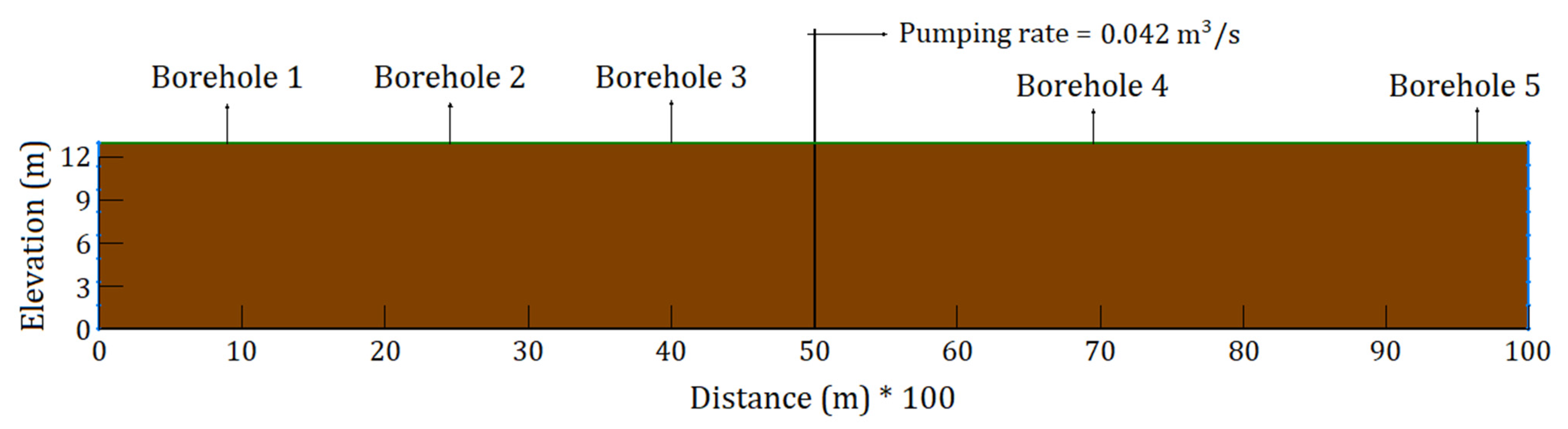
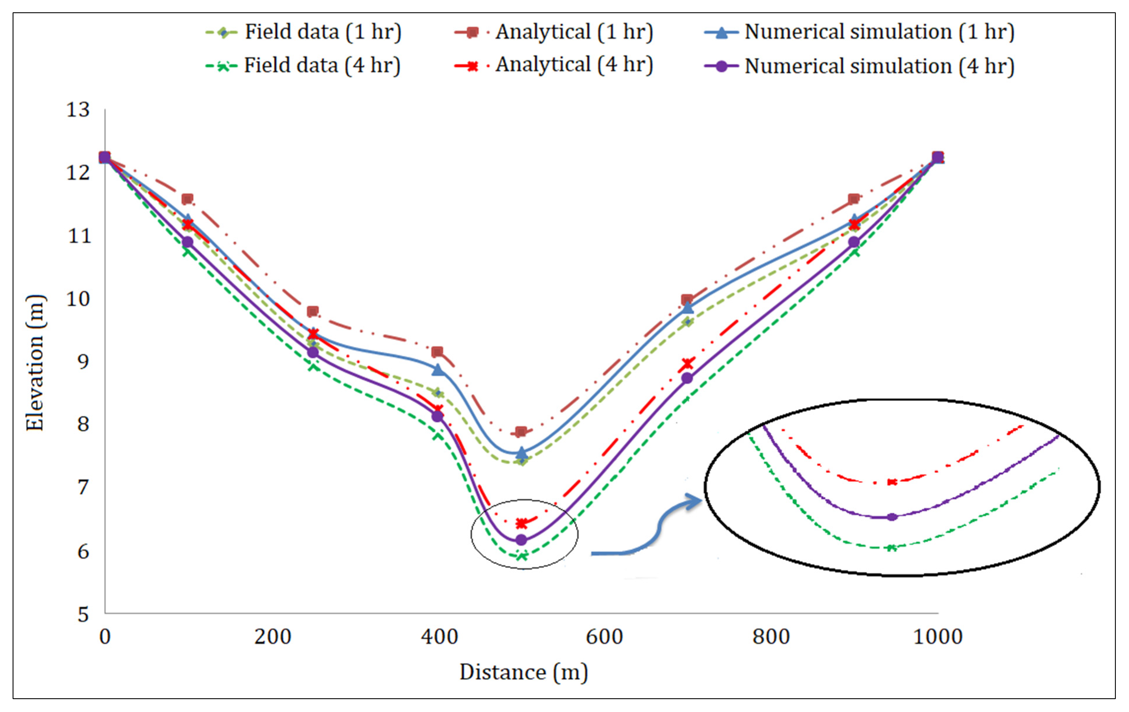
4.1. Verification of the Flow Model

Field experimental and analytical approach results, reported by Arshad et al. [38], were used as a test case to validate the performance of the numerical model to predict groundwater flow. According to the test case, sandy soil with five boreholes at distinct distances was simulated with the numerical model (Figure 2). The initial condition was obtained from a steady-state condition without pumping. Then, pumping at the rate of 0.042 m³/s was started, and results were obtained at a set of time intervals for the pumping well and all boreholes. The simulated drawdowns by the proposed model are in accordance with field data and an analytical approach, commonly known as the Theis equation [39] (Figure 3).

In order to evaluate the performance of the proposed numerical model for predicting the groundwater flow, mean absolute error (MAE), and root mean square error (RMSE) statistical indices were used in this research:

$$MAE=\frac{1}{n}{\displaystyle \sum }_{j=1}^n\left|H_{S{i}_j}-H_{O{b}_j}\right|$$

(15)

$$RMSE={\frac{\left[{{\displaystyle \sum }}_{j=1}^n{\left(H_{S{i}_j}-H_{O{b}_j}\right)}^2\right]}{{{\displaystyle \sum }}_{j=1}^n{H}_{O{b}_j}}}^{0.5}$$

(16)

where $H_{S{i}_j}$ is the jth value of the simulated head, and $H_{Obj}$ is the jth value of the observed head (field data). For the numerical model, $MAE$ and $RMSE$ values were found to be 0.19 m and 0.15, respectively. The comparison of both field experiments and analytical results with numerical simulation outcomes represents the perfect applicability of the numerical model.

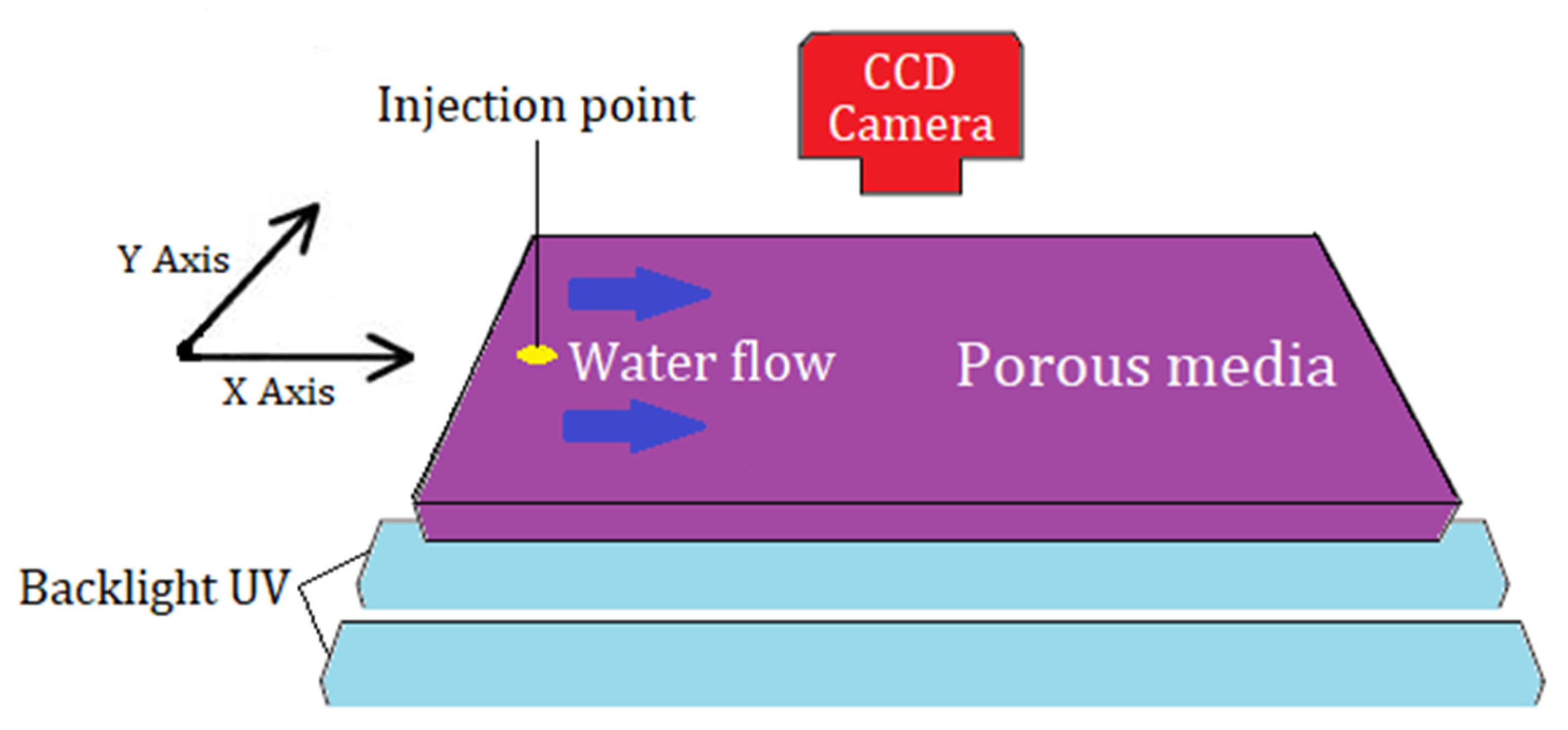
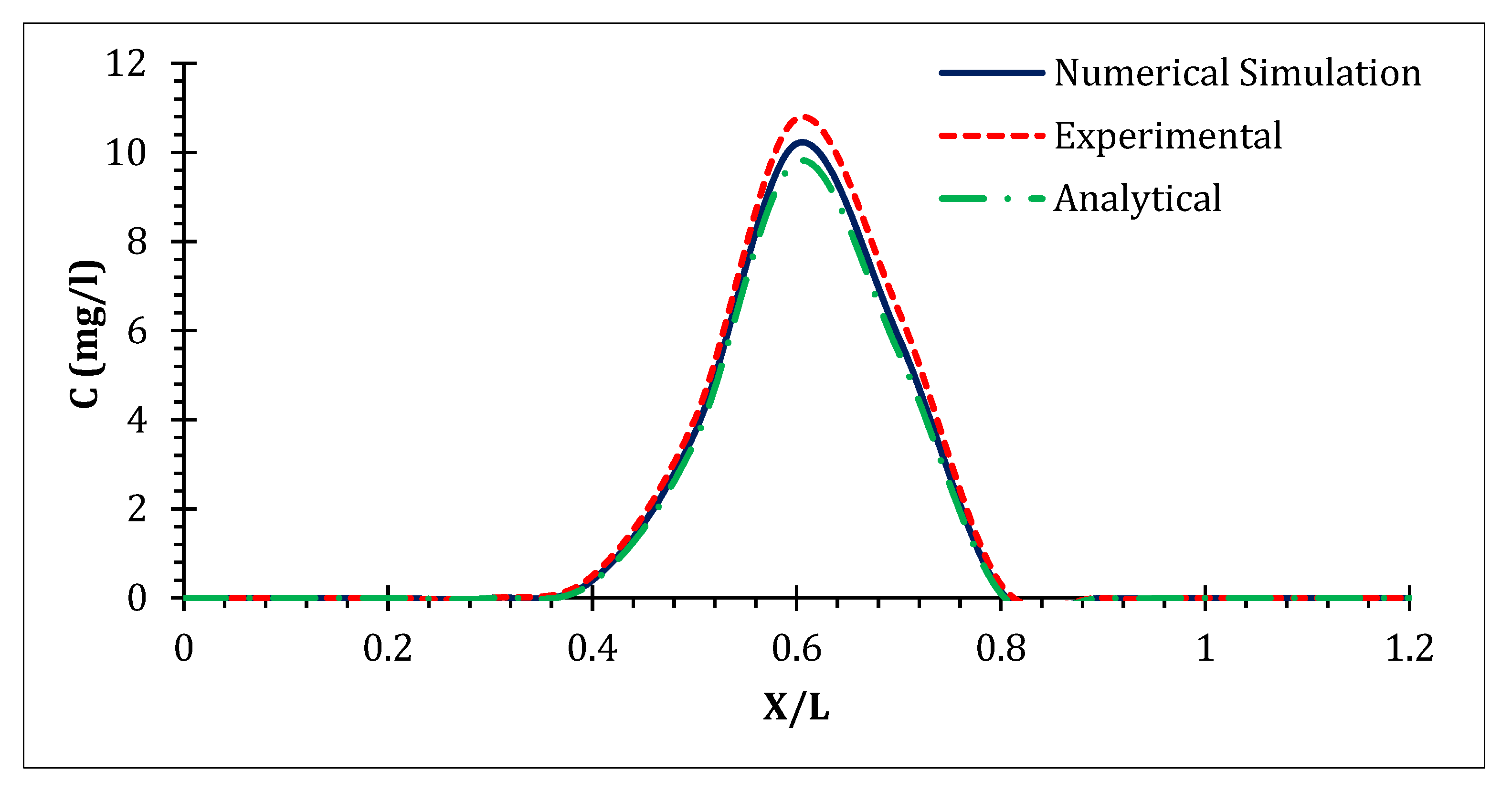
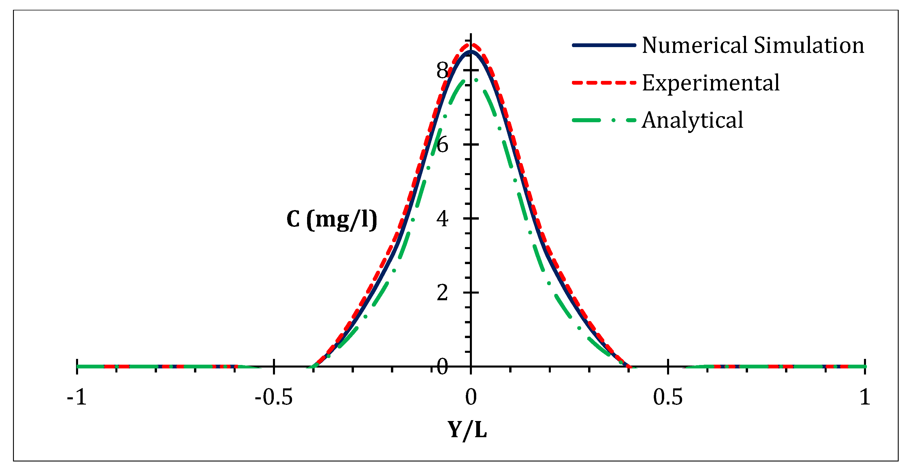
4.2. Verification of the Transport Model

The performance of the developed finite-volume model to predict the contaminant transport was validated by an experiment conducted by Massabo et al. [40]. The apparatus of the experiment mainly consisted of a chamber filled with glass beads to simulate contaminant migration through a semi-infinite saturated porous medium. The physical model can be regarded as quasi-2-dimensional because of its trivial thickness regarding the other dimensions of the experimental model. The solute was introduced by a pulse-like injection, and it was illuminated by a diffuse backlight UV source (Figure 4).

The analytical solution for simulating the contaminant transport through saturated porous media was presented by Ogata and Banks [41]. Comparisons among the numerical model, experimental data, and analytical solution are shown in Figure 5 and Figure 6. The curves in these figures are representative of the plume characteristics in the middle longitudinal cross section (y = 0) and at a fixed transverse cross section in the middle part of the longitudinal domain (x = 0.14 m) at time 400 s.

The accuracy of the simulation model was investigated by the mentioned statistical indices, and $MAE$ and $RMSE$ values were found to be 0.16 m and 0.14 m, respectively. Evaluation of experimental data and numerical simulation outcomes revealed that the numerical results had an acceptable agreement with both experimental and analytical results. The accordance indicates that the proposed model can adequately predict solute migration.

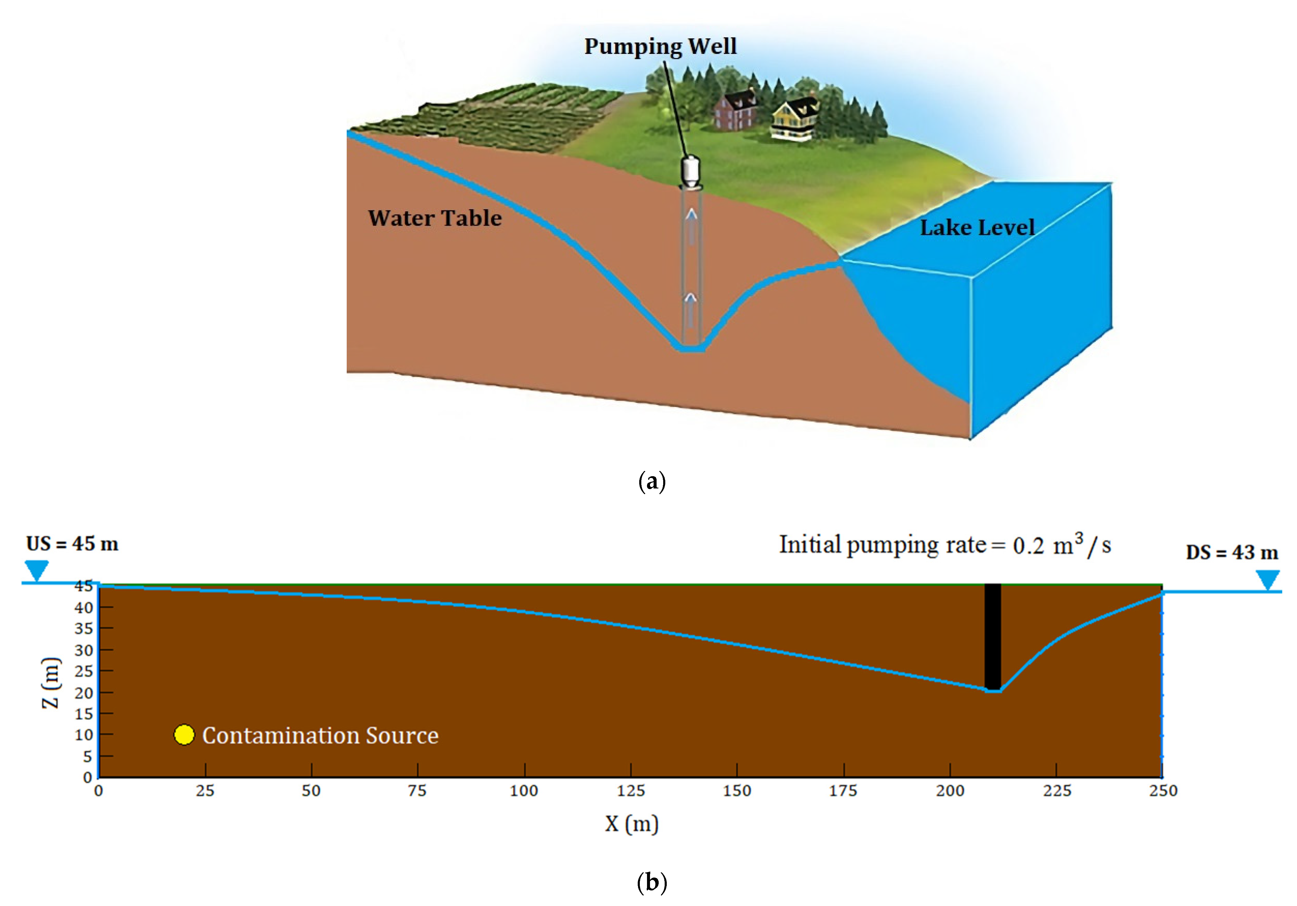
5. Numerical Implementation

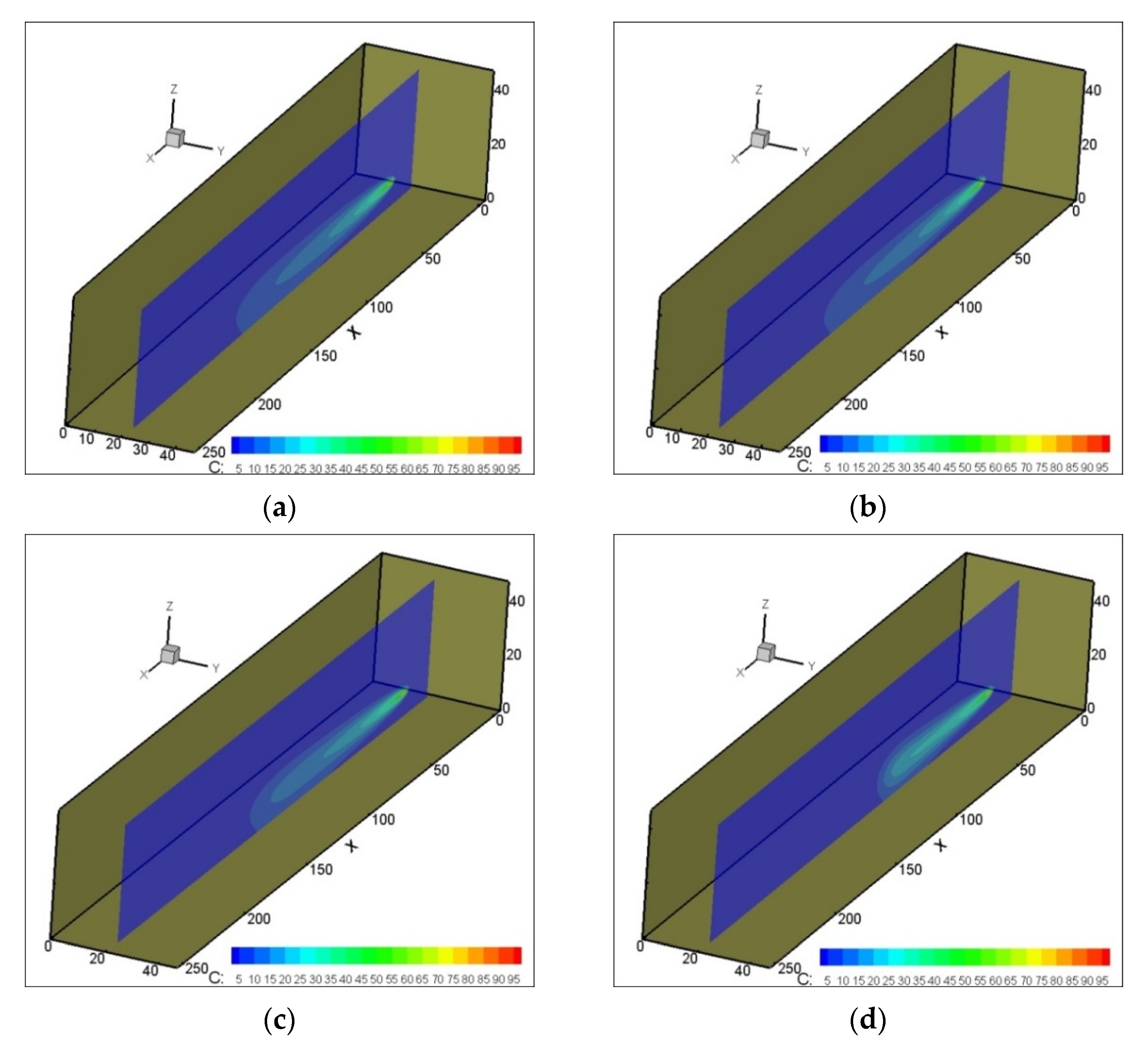
The proposed numerical model aims to investigate the impact of pumping rates on both groundwater flow and contamination transport through saturated porous media. At the beginning step, the proposed model simulated radial groundwater flow toward a pumping well to find the steady-state condition of groundwater flow. The steady state was obtained provided that groundwater flow parameters, such as piezometric heads, velocity, and pressure, did not change at any single point in the porous media. Then the pumping rate was changed, altering the groundwater flow properties and making the radial flow unsteady. The unsteady-state groundwater flow was simulated again to find a steady-state radial groundwater flow towards the pumping well; furthermore, the duration, through which the unsteady groundwater flow had converted to the steady-state condition, was simulated by the numerical model. The pollutant migration for each of the time steps, through and after the pumping rate change, was predicted.

This concept is illustrated by two hypothetical examples with a simplified homogeneous aquifer system, with $250\times 45\times 45 {\mathrm{m}}^3$ dimensions, including a single well or group of wells under the pumping rate of 0.2 ${\mathrm{m}}^3/\mathrm{s}$ (17,280 ${\mathrm{m}}^3/\mathrm{day}$). The upstream and downstream conditions for the examples are assumed to be fixed heads, which are 45 and 43 m respectively (Figure 7). The effect of the pumping rate on contaminant transport was investigated by considering four different pumping rate stages. These stages include 100%, 70%, 30% of the constant pumping rate, as well as ceasing the pumping. The pumping rate was changed from 100% to another rate as soon as the contaminant was injected into the porous media. The contaminant was injected into the porous media during a 24-h period. It should be noted that the model used a variable grid size to achieve ideal efficiency for the simulation of both groundwater flow and contaminant transport through saturated porous media. The grid size was reduced by half around the well to obtain maximum precision and flexibility.

The input variables and aquifer parameters are listed in

Table 1. Input variables and aquifer parameters of examples.

Parameter	Symbol	Value
Hydraulic conductivity	K	0.01 (m/s)
Average hydraulic gradient	i	0.008
Single well coordination	(Xsw, Ysw)	(210, 22.5)
Group of wells coordination	(Xgw, Ygw)	(210, 15), (210, 30)
Injection point	(X0, Y0, Z0)	(20, 22.5, 10)
Initial concentration	C0	100 (mg/L)
Injection time	T0	24 h.
Diffusion coefficient	D	${10}^{-6}$
Porosity	n	0.34

.

5.1. Single Well

In the first example, a single well in a homogeneous aquifer with a pumping rate of 0.2 ${\mathrm{m}}^3/\mathrm{s}$ was used to study the effects of pumping rate on contaminant transport. The four stages of the pumping rate were simulated by the numerical model, and the pollution plume for each of the pumping rates was obtained. The time taken to reach steady-state groundwater flow conditions, due to the pumping rate change from the initial pumping rate (100%) to 70% and 30%, as well as to cease the pumping were 28.4, 33.2, and 42.3 h, respectively. As mentioned earlier, once the solute contaminant, which had a constant concentration, was injected into the porous media, the pumping rate was changed from the initial pumping rate to another rate. Figure 8 and Figure 9 show the pollution plumes at the plane passing through the pumping well after 24 and 36 h, respectively.

Figure 8 and Figure 9 show that contaminant movement, as a result of groundwater flow, was a considerable process through the saturated porous media. This means the advection was the dominant process in the contaminant transport for all pumping rates; on the other hand, the ceased pumping case not only decelerated both advection and dispersion processes, but also made diffusion the predominant process in contaminant migration. Figure 10 shows the migration of the pollution under different pumping rates in the saturated porous media at the section passing through the well at $Z=10 \mathrm{m}$ over time.

The large velocity gradients attributed to the pumping conditions brought about faster advection and dispersion of the pollution; on the contrary, ceasing pumping considerably affected the groundwater flow, and dramatically reduced the velocity field through porous media, inducing a remarkable decrease in both advection and dispersion rates.

In Figure 11, the effect of the pumping rate on both travel time and contaminant concentrations for a single well is presented. Travel time is the time spent for contaminant arrival time at wells, and it directly depends upon the advection. In fact, travel time is a primary measure of the aquifer–solute contact time. The travel time is obtained from numerical simulations of transient flow and transport in the soil media.

In addition, the contaminant concentration at the well point varies with changing pumping rate. Figure 11 illustrates the pumping rate effect on the travel time, along with the maximum concentration at the well point over time.

Figure 11 indicates that as the single-well pumping rate reduces, the travel time negligibly increases, whereas ceasing pumping brings about a great growth in the travel time. Furthermore, by reducing the pumping rate from its initial rate to other rates, the peak of the contaminant concentration at the well point showed a gradual decline to reach its nadir; then it regrew. Decreasing the pumping rate increased the travel time for contaminants, whereby it prepared more time for contaminant dispersion. The difference in the travel time increase due to the reduction of the pumping rate was negligible; therefore, the effect of contaminant concentration reduction was slight. The greater the difference between the initial pumping rate and pumping rate reduction, the more time it took to reach the steady-state condition, with more advection and less dispersion. The final simulation of contaminant transport was related to ceasing pumping when the contaminant concentration at the point of the pumping well was greater than the pumping reduction stages. In this case, the velocity field significantly diminished; therefore, both advection and dispersion rates dwindled. Additionally, ceasing pumping made diffusion the dominant phenomenon in the contaminant transport process and triggered a travel time increase.

5.2. Group of Wells

In this section, the effect of the pumping rate for a group of two wells is investigated. The pumping rate of each well was 0.1 ${\mathrm{m}}^3/\mathrm{s}$, the sum of which equals the pumping rate of the last example. The time taken to reach steady-state groundwater flow, owing to the change of pumping rate from the initial pumping rate (100%) to 70%, 30%, and ceased pumping were 31.2, 38.5, and 54.1 h, respectively. The pollution plume at the section passing through the middle of both pumping wells for the four pumping stages after 24 h is shown in Figure 12. Note that the contaminant concentration in the group of wells case was similar to the single well case; however, the hydraulic conditions of the points were not the same.

Figure 13 indicates that advection was the dominant process in contaminant transport for all pumping stages; nevertheless, in the ceased pumping stage, both advection and dispersion rates were reduced. The pollution migration at the section through the middle of both wells and at $Z=10 \mathrm{m}$ under different pumping rates over time, is shown in Figure 13.

Figure 13 indicates that advection was the predominant phenomenon in pumping stages, and diffusion was the dominant process in the ceased pumping stage. Figure 14 shows the travel time of the group of wells, along with the contaminant concentration at the point located between the pumping wells.

As the figure shows, the travel time and the peak concentration at the point between two pumping wells were similar to the trend of the single well peak concentration because of the aforementioned reasons.

The time taken to reach steady-state groundwater flow conditions under different pumping rates is presented in

Table 2. Time to reach steady-state condition (hr.).

Reduction of Pumping Rate	Single Well	Group of Wells
100% to 70%	28.4	31.2
100% to 30%	33.2	38.5
100% to cease pumping	42.3	54.1

.

The case where a group of wells took a longer time to reach steady-state conditions, rather than the single well, was because of the interaction between the wells. A comparison between the pumping rate impact on both travel time and contaminant concentration for the single well and the group of wells is presented in Figure 15.

Based on Figure 15, the effect of the pumping rate change on the travel time, for both a single well and a group of wells, is the same. Therefore, the number of wells is not an overriding factor for determining contaminant travel time under various pumping rates. Conversely, it indicates that the peak of the contaminant concentration depends to a great extent on the number of wells, and it is intensified when the number of wells increases. The reason that the contaminant concentration in the group of wells condition increases is that, in this case, the pollution plume takes a longer time to reach the steady-state condition in comparison to the single well; consequently, the pollutant not only further conveys, but also disperses less. Unsteady duration is a period during which the hydraulic gradient and direction of groundwater flow dramatically change, which yields a high rate of advection. In the case of the group of wells, the advection rate was much higher than the advection rate in the single well case. Therefore, contaminant concentrations for the group of wells did not decrease as much as they did for the single well case.

6. Conclusions

In this study, a combined numerical model was presented to make accurate and precise simulations of both groundwater flow and contaminant transport in transient conditions through saturated porous media. Within the numerical model, unsteady governing equations were numerically solved by using the finite volume time splitting scheme. The performance and accuracy of the numerical models were successfully examined by several test cases, which indicated the current numerical model has enough capability to predict radial groundwater flow toward a pumping well and contaminant migration through aquifers, including advection, dispersion, and diffusion terms.

The effect of pumping rate on solute migration was evaluated by the numerical model, and the following results were drawn. The reduction in pumping rate was accompanied by a decrease in flow velocity, which decreased both the advection and dispersion rates, as well as the growth of contaminant travel time. Discontinuing the pumping brought about a dramatic drop in flow velocity, which induced a remarkable rise in travel time, along with an increase in pollution concentrations downstream.

Comparing the results of the single well with the group of wells revealed that the single well required less time to reach the steady-state groundwater flow condition, with the same inverse correlation between the travel time and the pumping rate in contaminant transport. By contrast, the effect of the pumping rate on the contaminant concentration was different. In fact, the peak contaminant concentration, as a result of the pumping rate reduction in the group of wells, was bigger than the single well case. The results illustrate that managing the pumping rate can yield reduced pollution at the well point. Thus, in order to minimize contamination, the optimum range for the pumping rate, which is attributed to the lowest well pollution, can be determined by numerical simulations.

References

1. Ayvaz, M.T. Identification of Pumping Well Characteristics in a Heterogeneous Aquifer System Using a Genetic Algorithm Approach. Ph.D. Thesis, Department of Civil Engineering, Pamukkale University, Denizli, Turkey, 2008. (In Turkish). [Google Scholar]
2. Karkush, M.O.; Kareem, Z.A. Investigation the impacts of fuel oil contamination on the behavior of passive piles group in clayey soils. Eur. J. Environ. Civ. Eng. 2018, 25, 485–501. [Google Scholar] [CrossRef]
3. Asfaw, D.; Ayalew, D. Modeling megech watershed aquifer vulnerability to pollution using modified DRASTIC model for sustainable groundwater management, Northwestern Ethiopia. Groundw. Sustain. Dev. 2020, 11, 100375. [Google Scholar] [CrossRef]
4. Chang, S.W.; Chung, I.M. Water Budget Analysis Considering Surface Water–Groundwater Interactions in the Exploitation of Seasonally Varying Agricultural Groundwater. Hydrology 2021, 8, 60. [Google Scholar] [CrossRef]
5. Ducci, D.; Sellerino, M. Vulnerability mapping of groundwater contamination based on 3D lithostratigraphical models of porous aquifers. Sci. Total Environ. 2013, 447, 315–322. [Google Scholar] [CrossRef]
6. Medici, G.; Baják, P.; West, L.J.; Chapman, P.J.; Banwart, S.A. DOC and nitrate fluxes from farmland; impact on a dolostone aquifer KCZ. J. Hydrol. 2021, 595, 125658. [Google Scholar] [CrossRef]
7. Massabo, M.; Cianci, R.; Paladino, O. Some analytical solutions for two-dimensional convection–dispersion equation in cylindrical geometry. Environ. Model. Softw. 2006, 21, 681–688. [Google Scholar] [CrossRef]
8. Wu, X.; Shi, J.; He, J. Analytical solutions for diffusion of organic contaminant through composite liner considering degradation in leachate and soil liner. Int. J. Environ. Pollut. 2017, 61, 166–185. [Google Scholar] [CrossRef]
9. Mustafa, S.; Darwish, M.; Bahar, A.; Aziz, Z.A. Analytical Modeling of Well Design in Riverbank Filtration Systems. Groundwater 2019, 57, 756–763. [Google Scholar] [CrossRef]
10. Kim, S.B. Numerical analysis of bacterial transport in saturated porous media. Hydrol. Process. Int. J. 2006, 20, 1177–1186. [Google Scholar] [CrossRef]
11. Malaguerra, F.; Albrechtsen, H.J.; Binning, P.J. Assessment of the contamination of drinking water supply wells by pesticides from surface water resources using a finite element reactive transport model and global sensitivity analysis techniques. J. Hydrol. 2013, 476, 321–331. [Google Scholar] [CrossRef]
12. Ben-Zvi, R.; Jiang, S.; Scher, H.; Berkowitz, B. Finite-Element Method Solution of Non-Fickian Transport in Porous Media: The CTRW-FEM Package. Groundwater 2019, 57, 479–484. [Google Scholar] [CrossRef]
13. Gkiougkis, I.; Pouliaris, C.; Pliakas, F.K.; Diamantis, I.; Kallioras, A. Conceptual and Mathematical Modeling of a Coastal Aquifer in Eastern Delta of R. Nestos (N. Greece). Hydrology 2021, 8, 23. [Google Scholar] [CrossRef]
14. Maqsood, I.; Luo, B. Integrated 3D physical-numerical modelling for simulating bioremediation of petroleum contamination in heterogeneous subsurface environment. Int. J. Environ. Pollut. 2010, 42, 199–219. [Google Scholar] [CrossRef]
15. Meenal, M.; Eldho, T.I. Meshless Point Collocation Method for 1D and 2D groundwater flow simulation. ISH J. Hydraul. Eng. 2011, 17, 71–87. [Google Scholar] [CrossRef]
16. Navas, P.; López-Querol, S.; Yu, R.C.; Li, B. B-bar based algorithm applied to meshfree numerical schemes to solve unconfined seepage problems through porous media. Int. J. Numer. Anal. Methods Geomech. 2016, 40, 962–984. [Google Scholar] [CrossRef]
17. Ahmadi, H. An implicit numerical model for solving free-surface seepage problems. ISH J. Hydraul. Eng. 2021, 1–9. [Google Scholar] [CrossRef]
18. Ahmadi, H. A numerical scheme for advection dominated problems based on a Lagrange interpolation. Groundw. Sustain. Dev. 2021, 13, 100542. [Google Scholar] [CrossRef]
19. Ahmadi, H.; Namin, M.M.; Kilanehei, F. Development a numerical model of flow and contaminant transport in layered soils. Adv. Environ. Res. 2016, 5, 263–282. [Google Scholar] [CrossRef]
20. Halford, K.J.; Stamos, C.L.; Nishikawa, T.; Martin, T. Arsenic management through well modification and simulation. Groundwater 2010, 48, 526–537. [Google Scholar] [CrossRef]
21. Johnson, R.L.; Clark, B.R.; Landon, M.K.; Kauffman, L.J.; Ebert, S.M. Modeling the potential impact of seasonal and inactive multi-aquifer wells on contaminant movement to public water supply wells. J. Am. Water Resour. Assoc. 2011, 47, 588–596. [Google Scholar] [CrossRef]
22. Park, C.H.; Aral, M.M. Multi-objective optimization of pumping rates and well placement in coastal aquifers. J. Hydrol. 2004, 290, 80–99. [Google Scholar] [CrossRef]
23. Kalwij, I.M.; Peralta, R.C. Simulation/optimization modeling for robust pumping strategy design. Groundwater 2006, 44, 574–582. [Google Scholar] [CrossRef]
24. Zinn, B.A.; Konikow, L.F. Effects of intraborehole flow on groundwater age distribution. Hydrogeol. J. 2007, 15, 633–643. [Google Scholar] [CrossRef]
25. Sharief, S.M.V.; Eldho, T.I.; Rastogi, A.K. Optimal pumping policy for aquifer decontamination by pump and treat method using genetic algorithm. ISH J. Hydraul. Eng. 2008, 14, 1–17. [Google Scholar] [CrossRef]
26. Bexfield, L.M.; Jurgens, B.C. Effects of Seasonal Operation on the Quality of Water Produced by Public-Supply Wells. Groundwater 2014, 52, 10–24. [Google Scholar] [CrossRef] [PubMed] [Green Version]
27. Cyriac, R.; Rastogi, A.K. Optimization of pumping policy using coupled finite element-particle swarm optimization modelling. ISH J. Hydraul. Eng. 2016, 22, 88–99. [Google Scholar] [CrossRef]
28. Rodriguez-Pretelin, A.; Nowak, W. Dynamic re-distribution of pumping rates in well fields to counter transient problems in groundwater production. Groundw. Sustain. Dev. 2019, 8, 606–616. [Google Scholar] [CrossRef]
29. Dey, S.; Prakash, O. Managing saltwater intrusion using conjugate sharp interface and density dependent models linked with pumping optimization. Groundw. Sustain. Dev. 2020, 11, 100446. [Google Scholar] [CrossRef]
30. Medici, G.; West, L.J.; Chapman, P.J.; Banwart, S.A. Prediction of contaminant transport in fractured carbonate aquifer types: A case study of the Permian Magnesian Limestone Group (NE England, UK). Environ. Sci. Pollut. Res. 2019, 26, 24863–24884. [Google Scholar] [CrossRef] [Green Version]
31. Medici, G.; West, L.J. Groundwater flow velocities in karst aquifers; importance of spatial observation scale and hydraulic testing for contaminant transport prediction. Environ. Sci. Pollut. Res. 2021, 1–14. [Google Scholar] [CrossRef]
32. Bear, J. Hydraulics of Groundwater; McGraw-Hill: New York, NY, USA, 1979. [Google Scholar]
33. Schulze-Makuch, D. Longitudinal Dispersivity Data and Implications for Scaling Behavior. Groundwater 2005, 14, 43–52. [Google Scholar] [CrossRef] [PubMed]
34. Bear, J.; Verruijt, A. Modeling Groundwater Flow and Pollution; Springer Science and Business Media: Berlin/Heidelberg, Germany, 2012; Volume 2. [Google Scholar]
35. Zech, A.; Attinger, S.; Bellin, A.; Cvetkovic, V.; Dietrich, P.; Fiori, A.; Teutsch, G.; Dagan, G. A Critical Analysis of Transverse Dispersivity Field Data. Groundwater 2019, 57, 632–639. [Google Scholar] [CrossRef]
36. Yanenko, N.N. The Method of Fractional Steps; Springer: Berlin/Heidelberg, Germany, 1971. [Google Scholar] [CrossRef]
37. Namin, M.M.; Falconer, R.A. An efficient coupled 2-DH and 3D hydrodynamic model for river and coastal application. In Hydroinformatics; World Scientifc: Singapore, 2008; pp. 374–382. [Google Scholar] [CrossRef]
38. Arshad, I.; Baber, M.M. Finite element analysis of seepage through an earthen dam by using geo-slope (SEEP/W) software. Int. J. Res. 2014, 1, 612–619. [Google Scholar]
39. Theis, C.V. The relation between the lowering the piezometric surface and the rate and duration of discharge of a well using Ground-Water storage. Trans. Am. Geophys. Union 1935, 16, 519–524. [Google Scholar] [CrossRef]
40. Massabo, M.; Cianci, R.; Paladino, O. An Analytical Solution of the Advection Dispersion Equation in a Bounded Domain and Its Application to Laboratory Experiments. J. Appl. Math. 2011, 23, 90–104. [Google Scholar] [CrossRef]
41. Ogata, A.; Banks, R.B. A Solution of the Differential Equation of Longitudinal Dispersion in Porous Media: Fluid Movement in Earth Materials; US Government Printing Office: Washington, DC, USA, 1961; Volume 411. [CrossRef] [Green Version]
Figure 1. The grid layout of the 3-D calculation domain of porous media and variables’ positions.
Hydrology 08 00103 g001
Figure 2. Two-dimensional domains of the field experiment.
Hydrology 08 00103 g002
Figure 3. Comparison of field data, analytical, and numerical piezometric heads.
Hydrology 08 00103 g003
Figure 4. A schematization of the experimental model and imaging setup.
Hydrology 08 00103 g004
Figure 5. Comparison between numerical simulation and experimental data, fixed longitudinal cross section at y = 0.
Hydrology 08 00103 g005
Figure 6. Comparison between numerical simulation and experimental data, fixed transverse cross section at x = 0.14.
Hydrology 08 00103 g006
Figure 7. The conceptual domain of considered examples: (a) 3D view and (b) positions of the single well and the contamination source at cross sections, perpendicular to the y-axis (at Y = 22 m).
Hydrology 08 00103 g007
Figure 8. Contaminant plumes at cross sections passing through a single well after 24 h: (a) 100% pumping, (b) 70% pumping, (c) 30% pumping, and (d) ceased pumping.
Hydrology 08 00103 g008
Figure 9. Contaminant plume at cross sections passing through a single well after 36 h: (a) 100% pumping, (b) 70% pumping, (c) 30% pumping, and (d) ceased pumping.
Hydrology 08 00103 g009
Figure 10. Contaminant concentrations for a single-well at cross sections passing through the single well at Z = 10 m: (a) 100% pumping, (b) 70% pumping, (c) 30% pumping, and (d) ceased pumping.
Hydrology 08 00103 g010aHydrology 08 00103 g010b
Figure 11. The pumping rate effect on the travel time for single-well.
Hydrology 08 00103 g011
Figure 12. Contaminant plume at the section passing through the middle of both pumping wells after 24 h: (a) 100% pumping, (b) 70% pumping, (c) 30% pumping, and (d) ceased pumping.
Hydrology 08 00103 g012
Figure 13. Contaminant migration for a group of wells: (a) 30% pumping and (b) ceased pumping.
Hydrology 08 00103 g013
Figure 14. The pumping rate effect on the travel time for a group of wells.
Hydrology 08 00103 g014
Figure 15. Comparison of the pumping rate effect on travel time and contaminant concentration.
Hydrology 08 00103 g015