A Model-Based Tool for Assessing the Impact of Land Use Change Scenarios on Flood Risk in Small-Scale River Systems—Part 1: Pre-Processing of Scenario Based Flood Characteristics for the Current State of Land Use

Abstract

Land use changes influence the water balance and often increase surface runoff. The resulting impacts on river flow, water level, and flood should be identified beforehand in the phase of spatial planning. In two consecutive papers, we develop a model-based decision support system for quantifying the hydrological and stream hydraulic impacts of land use changes. Part 1 presents the semi-automatic set-up of physically based hydrological and hydraulic models on the basis of geodata analysis for the current state. Appropriate hydrological model parameters for ungauged catchments are derived by a transfer from a calibrated model. In the regarded lowland river basins, parameters of surface and groundwater inflow turned out to be particularly important. While the calibration delivers very good to good model results for flow (E_vol =2.4%, R = 0.84, NSE = 0.84), the model performance is good to satisfactory (E_vol = −9.6%, R = 0.88, NSE = 0.59) in a different river system parametrized with the transfer procedure. After transferring the concept to a larger area with various small rivers, the current state is analyzed by running simulations based on statistical rainfall scenarios. Results include watercourse section-specific capacities and excess volumes in case of flooding. The developed approach can relatively quickly generate physically reliable and spatially high-resolution results. Part 2 builds on the data generated in part 1 and presents the subsequent approach to assess hydrologic/hydrodynamic impacts of potential land use changes.

1. Introduction

1.1. Background

Flooding is a natural and recurring phenomenon. It ensures fertile floodplains and therefore favors agriculture in river valleys. Besides, the use of rivers as transport routes for trade promoted human settlement along the waterways. However, for both reasons, land cultivation and water transport, rivers and streams have often been straightened [1]. In parallel, population growth is inevitably accompanied by increasing land sealing, which in turn accelerates surface runoff [2,3,4] at the expense of evaporation and infiltration. In Italy, for example, an average increment of 8.4% in soil sealing induced an average increase in surface runoff equal to 3.5% and 2.7% respectively for 20- and 200-year return periods [5]. Increased surface runoff, flow course shortening, or deformation and loss of retention space are drivers for raising peak flows and increased flood probabilities. These factors are superimposed by changing hydro-meteorological conditions due to climate [6,7,8]. Accordingly, responsible development of land use should also take the resulting impact on river runoff and flood probability into account. This requires a sound understanding of the hydrological and hydrodynamic processes in the regarded catchment and the affected river basin.

The term flood risk is always related to the probability or recurrence interval of a certain runoff or water table. Generally, these values can be derived via three ways:

(1)

Statistical analysis of historic time series.

(2)

Statistical regionalization of flood characteristics.

(3)

Hydrologic modeling (if a water table is required, supplemented by hydrodynamic models).

Time series analysis requires the availability of monitoring data of flow and/or water table over a sufficient long observation period (10 a minimum, 30 a or more is better [9]). Since monitoring stations are maintenance-intensive and costly, those data are only available for a very limited number of rivers or river sections. Smaller streams and tributaries tend not to be surveyed at all.

To close this data gap, various procedures for regionalizing flood parameters are in use. Most of them are based on observed discharges in similar regions. Simple methods are related solely on the size of the catchment and assume the same discharge per area at the location with measurement and at the location without measurement. Further development of this is the multiple regression, which links several relevant basin parameters (e.g., basin size, slope, flow length, basin shape, soil, and geology parameters) to peak discharge. There are a number of other procedures, yet these will not be considered further here. Statistical regionalization methods are relatively simple to apply and require comparatively little time, which is why they are justifiably utilized in practice for certain questions.

The third option is to employ (regionalized) hydrologic models to predict runoff from ungauged watersheds, with the objective of relating various model parameters to the physical characteristics of the watershed [10,11]. Models used in this context are usually conceptual, lumped models, describing the runoff process in a simplified way, based on comparatively few model parameters. Influencing factors and thus significant model parameters differ from region to region and depend on the dominant hydrological processes in the respective catchment region and on the desired result (e.g., peak flows vs. average monthly or annual flow values). A study conducted in the Ivory Coast marked that land use and rainfall distribution over the year are important model parameters in the context of regionalization [12]. The role of precipitation was also highlighted by a study from Australia using a monthly water balance model, where the mean annual precipitation at different locations ranged from 600 mm to 2400 mm [13]. However, this shows that model results are also sensitive to the precipitation characteristics, which is actually an input variable.

Astonishingly, deterministic models with a clear conceptual link between physical conditions in the catchment and the resulting hydrologic processes have been rarely applied in ungauged systems, probably mainly due parametrization questions. However, namely process-oriented semi or fully distributed models should be well suitable for those situations provided that the physical data can be derived from geodata or remote sensing. This would allow for physically funded parameter transfer from modeling studies with calibration data. A corresponding study dedicated to flash floods achieved only a small decrease of performance of 10% by transferring calibrated model parameters to a new validation site [14].

None of the studies mentioned above consider river or stream hydraulics, which is of particular importance in the formation of flood flows. In particular, small rivers in cultivated or urbanized areas are modified by man-made structures such as culverts and pipelines, which have a significant influence on flow dynamics and water level. Leading back to the initial problem of analyzing future land use changes on stream hydraulics, deterministic models should also provide a hydrodynamic functionality, requiring additional physical data, i.e., river profiles and infrastructural data.

Meanwhile, in many parts of the world, the availability and quality of hydrologically and hydrodynamically relevant geodata (soil type, land use, DEM, groundwater levels, etc.) is very good. Setup and parametrization of physically based models directly based on these data should therefore be more and more possible.

However, this concept has a clear constraint: The application of those models, even if well parametrized, is hardly applicable by regional planners who are typically not modeling experts. When providing those models for regional planning purposes, they must be tailored for the envisaged group of end-users. A promising way to do so is the combination model setup, parametrization and preprocessing for the status quo with a simplified GIS-based analysis for land-use change scenarios.

1.2. Objectives and Structure of the Study

Summing up the arguments above, the overall objective of this study is twofold:

(4)

To develop a concept to setup and parametrize a deterministic distributed model based on available geodata.

(5)

To develop a simplified algorithm for analyzing land-use change scenarios that is based on the models developed but can be used by regional planning practitioners.

Following these targets, the study is separated into two papers. Part 1 is dedicated to model setup and parametrization and the determination of flood characteristics for the current state and thus forms the basis for the second part. The innovative approach of the method presented lies in the automated transfer of physical model parameters based on geodata for the use of spatially and temporally highly resolved deterministic rainfall runoff and stream models. The desired results can be generated comparatively fast but are, at the same time, physically validated.

Part 2 will describe the developed simplified procedure for the rapid calculation of land use change effects on flood characteristics and its embedding in a GIS-based decision support system (reference to part 2).

2. Materials and Methods

2.1. Study Area and Data Used

The study area is located in the northeast of Germany and covers approximately 530 km². It comprises the city of Rostock and its neighbouring municipalities (see Figure 1) and contains more than 1500 km of small tributaries that drain into the Warnow or directly into the Baltic Sea. In order to achieve a high spatial resolution in the model setup and to maintain an overview in the process, the study area was divided into several smaller catchments.

Although the catchments are located close to each other and are subject to very similar climatic conditions, they differ in some characteristics. For example, the landscape in the south-east is relatively hilly, while the catchments near the Baltic Sea are rather flat. The catchments within the city have a high proportion of sealed surfaces, while agricultural land use dominates in the surrounding municipalities.

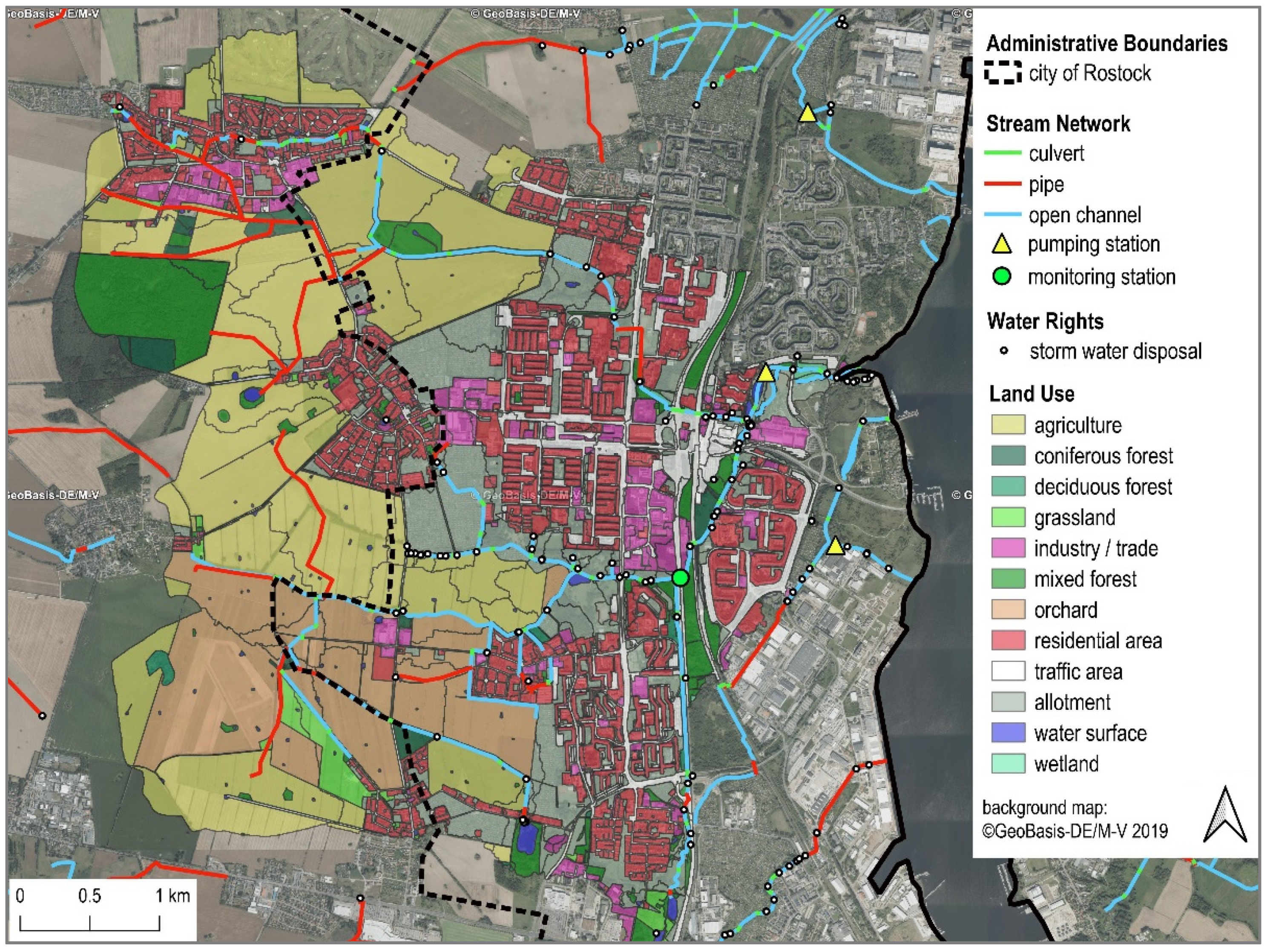
For model calibration, the Schmarler Bach catchment was used (Figure 2) as continuous flow and water level measurement data had already been collected here [15]. The 23 km² area has little gradient and is therefore one of the flat representatives (−1 m–30 m above sea level). A pumping station keeps the water level in the lower reaches below the level of the Baltic Sea. Approximately 34% of the area is partially impervious, which is due to urban use (residential area, traffic area, and industry/trade) [16]. The second largest share is arable land with 29 %. With intensive urban use, the number of storm water disposals increases. At Schmarler Bach, there are a total of 91 points, which is the largest number compared to the other model sites.

The monitoring station is located in the southern branch of the stream network. Its catchment is about 12 km² in size and is already significantly influenced by urban use.

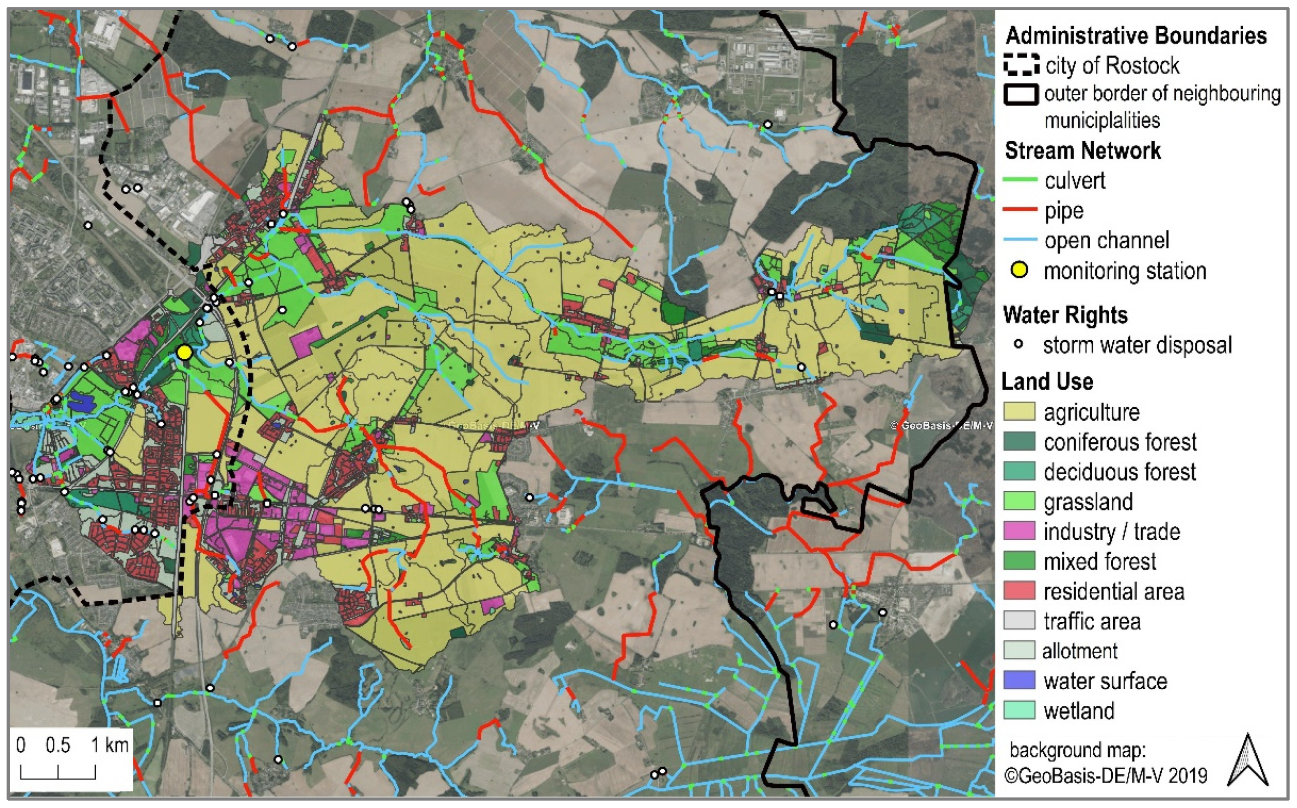
The catchment of the Carbäk stream was used for testing the concept of parameter transfer based on geodata without additional calibration (Figure 3). With its 42 km², it is about twice as large as the Schmarler Bach catchment. Due to the large east–west extension, the surface elevations span between 0 m to 65 m above sea level and thus show a comparatively larger range. Differences can be noted in land use patterns: While arable land takes up more than 50% of the area, partial sealed uses are only represented by 18 %. Accordingly, there are fewer storm water disposals to count (44 in total). The catchment of the monitoring station is 33 km² in size and thus almost 3 times larger than the catchment of the monitoring station in the Schmarler Bach.

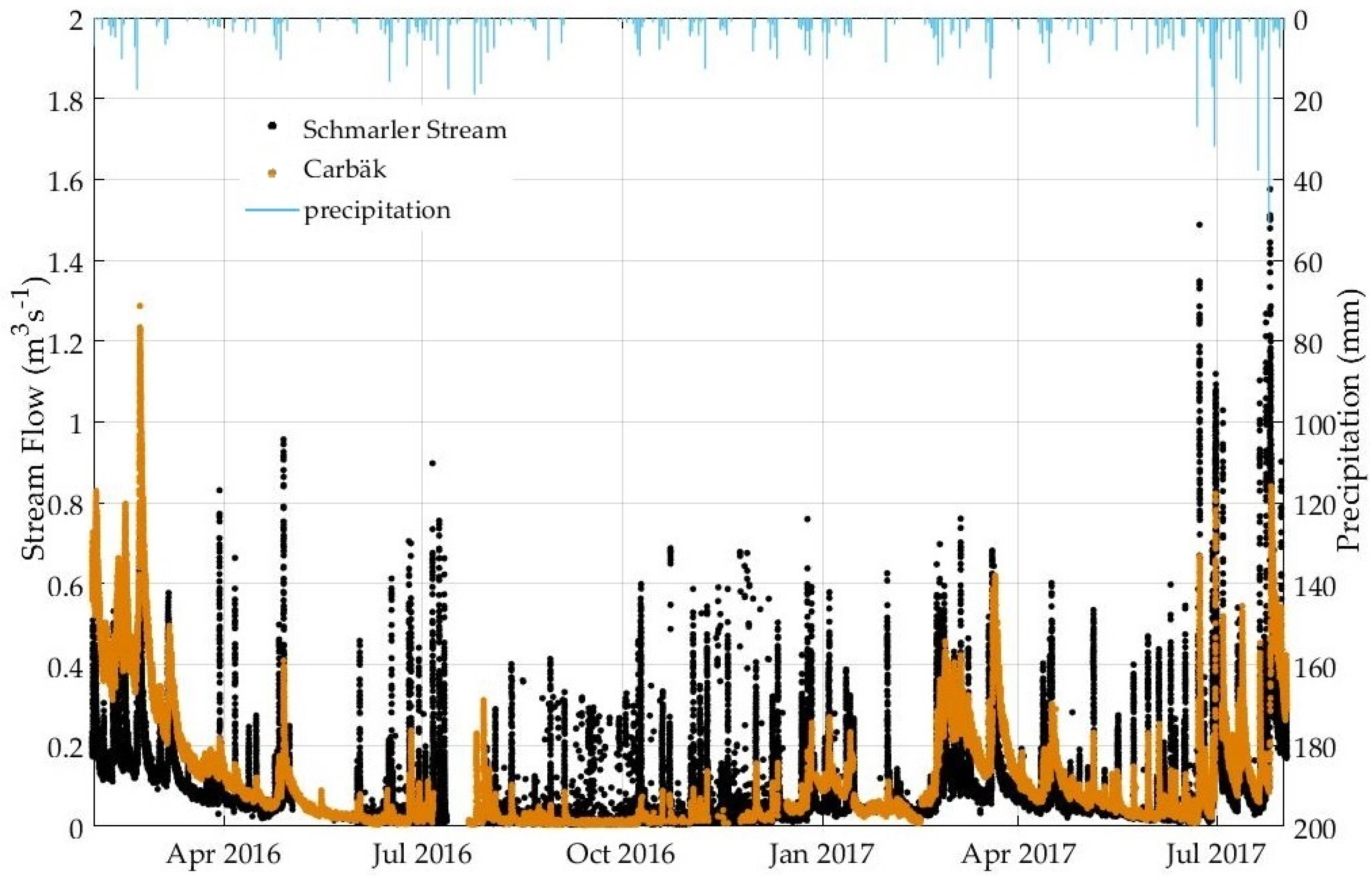
Figure 4 compares the measured flows of the two monitoring stations and illustrates the daily sums of rainfall of the rain gauge “Uni Rostock Hy” (the University of Rostock, department of hydrology and applied meteorology). Schmarler Bach flows show high peaks in the summer months, especially in wet June and July 2017, which is due to intensive rainfall and the large proportion of sealed areas that provoke a high amount of direct (and fast) runoff. In contrast, the Carbäk shows the highest flows generally in winter and spring and also in the extraordinary wet month June/July 2017. This suggests that the source of high flows in the Carbäk catchment are different from those in the Schmarler Bach. Since the Carbäk catchment is intensively farmed and drained, the high flows can be attributed to agricultural tile drainage interflows. These occur in the stream when the surrounding soil is saturated, which is usually the case when more rain falls than evapotranspirates. As these interflows have to pass through the soil to enter the drainage network, they require more time compared to surface runoff, which results in a stretched, flattened course of discharges.

2.2. Data Processing and Modelling Software

The basis for further work is the homogenization of geodata, which was carried out using QGIS (version 3.10.2) [17,18]. The attributes of the homogenized geodata are further processed with the help of a spreadsheet program. Here, Microsoft (MS) Excel was used together with its Visual Basic for Applications (VBA) interface [19]. VBA contributes to automation and enables faster processing of repetitive tasks. A free alternative to MS Excel is LibreOffice Calc [20], which also provides a VBA interface, but with limited macro support.

Prior to actual model development, a thorough review of available modelling software tools was performed. There is a wide range of hydrologic models with different pros and cons (cf. [21]). For the purposes of this study, the software should fulfill the following criteria:

• Freeware for wide transferability and applicability.
• Combined representation of rainfall-runoff and hydrodynamic streamflow processes to avoid external coupling of different models.
• Physically based, parameters widely derivable from geodata.
• Sufficient spatial distribution, capable to allocate distinct land use changes in the regarded river basin.
• Easy and automatable setup and parametrization of the model.

Namely, the required hydrodynamic functionality is rarely available. After a first screening, the combination of HEC-HMS [22] with HEC-RAS [23] and SWMM-UrbanEVA [24], an extension of the widely used software SWMM, were the most promising candidates. The UrbanEVA upgrade involves the implementation of vegetation-specific evapotranspiration and its reduction by a shading factor in the case of urban shading. A detailed description can be found in [16,24]. In a following detailed comparison, the decision was made in favor of SWMM-UrbanEVA.

SWMM (storm water management model [25]) was originally developed for the simulation and evaluation of storm runoff and sewer hydraulics in urban areas [26]. However, with the extension for evapotranspiration calculation, SWMM is very well suited for the simulation of near-natural catchments outside urban areas [16]. The calculation of water balance variables and streamflow is largely physically based. The SWMM input file is a simple text file that can be opened, read, and modified in any text editor, which facilitates an automated model generation. One of the biggest advantages of SWMM is that it combines both a hydrological rainfall-runoff model and a hydrodynamic drainage model in one software, which makes the numerical calculation very effective and stable, since no external coupling is needed.

2.3. The General Concept

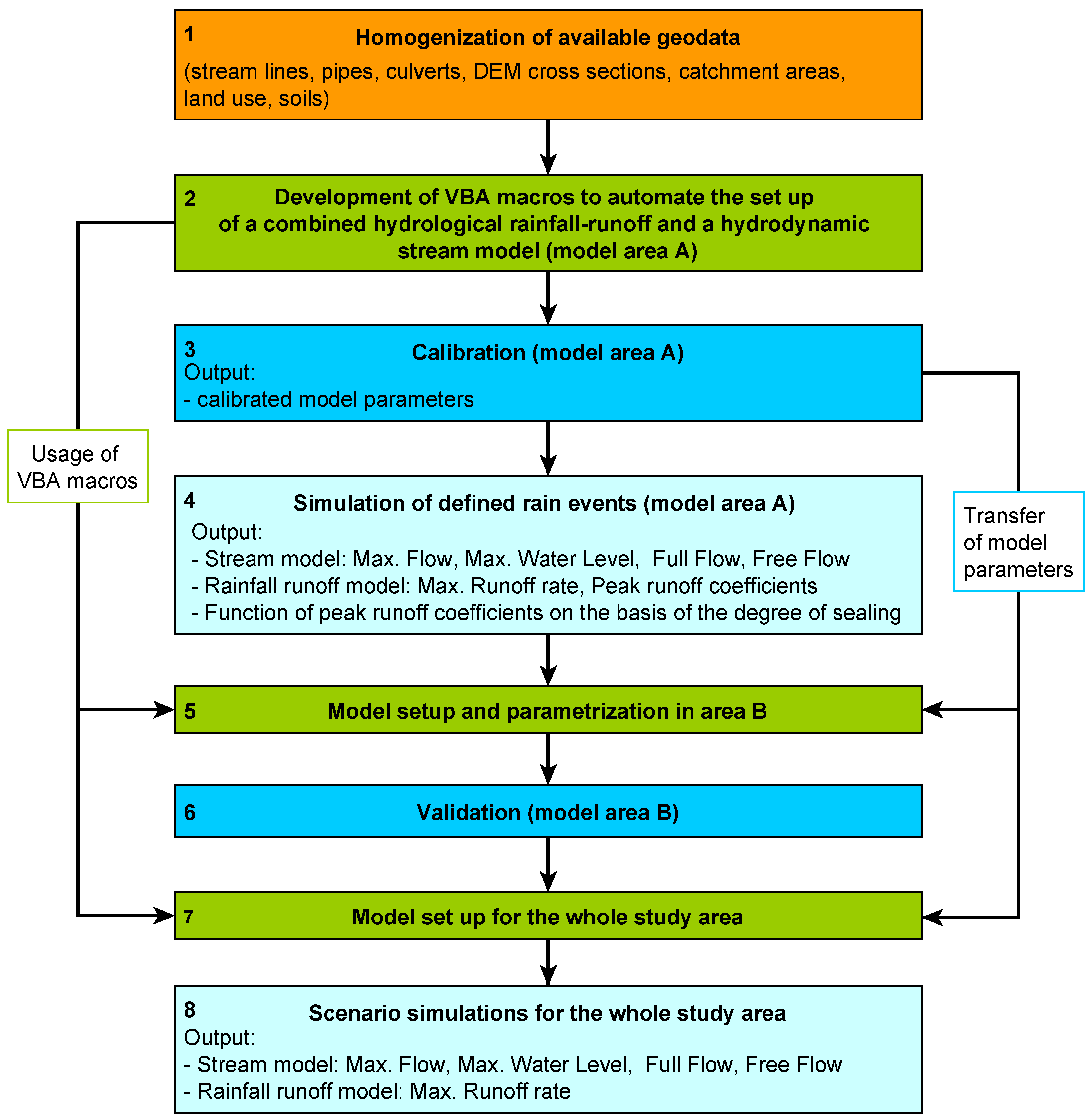
In order to obtain flood characteristics for the actual state of land use, a method was developed that consists of several steps, each involving the use of different software tools (Figure 5). The individual steps are described in detail in the following subsections.

2.4. Homogenization of Available Geodata

In the first step, geodata are homogenized so that uniform datasets without gaps are available for the entire study area. The necessary sub-steps for this were carried out with QGIS.

Table 1. Geodata used for the setup of the SWMM-UrbanEVA model (WIN = hierarchical watercourse identification number).

Available Geodata	Format	Attributes Derived for SWMM
hydrodynamic stream model
open channel segments	vector (line)	WIN, chainage, positioning
watercourse routes	vector (line) with measures	WIN, chainage, positioning
Pipes, culverts	vector (line)	chainage, diameter, material (roughness)
storm water disposals (water rights)	vector (points)	diameter, material (roughness)
DEM_0.2	raster (0.2 m resolution)	stream cross sections/transects
DEM_5	raster (5 m resolution)	ground elevation above pipes, culverts and storm water disposals
rainfall-runoff model
surface catchments for 50 m-stream segments	vector (polygon)	area size, flow length, outlet (computation node of hydrodynamic model)
land use maps	vector (polygon)	generalized land use types, leaf area index, crop factor, detention storage, roughness
groundwater isohypses	vector (lines)	average groundwater level for each subcatchment
soil maps	vector (polygon)	conductivity, porosity, field capacity, wilting point
DEM_5	raster (5 m resolution)	average slope
soil sealing maps	raster (10 m resolution)	degree of sealing

provides an overview of the data used and the attributes derived from it.

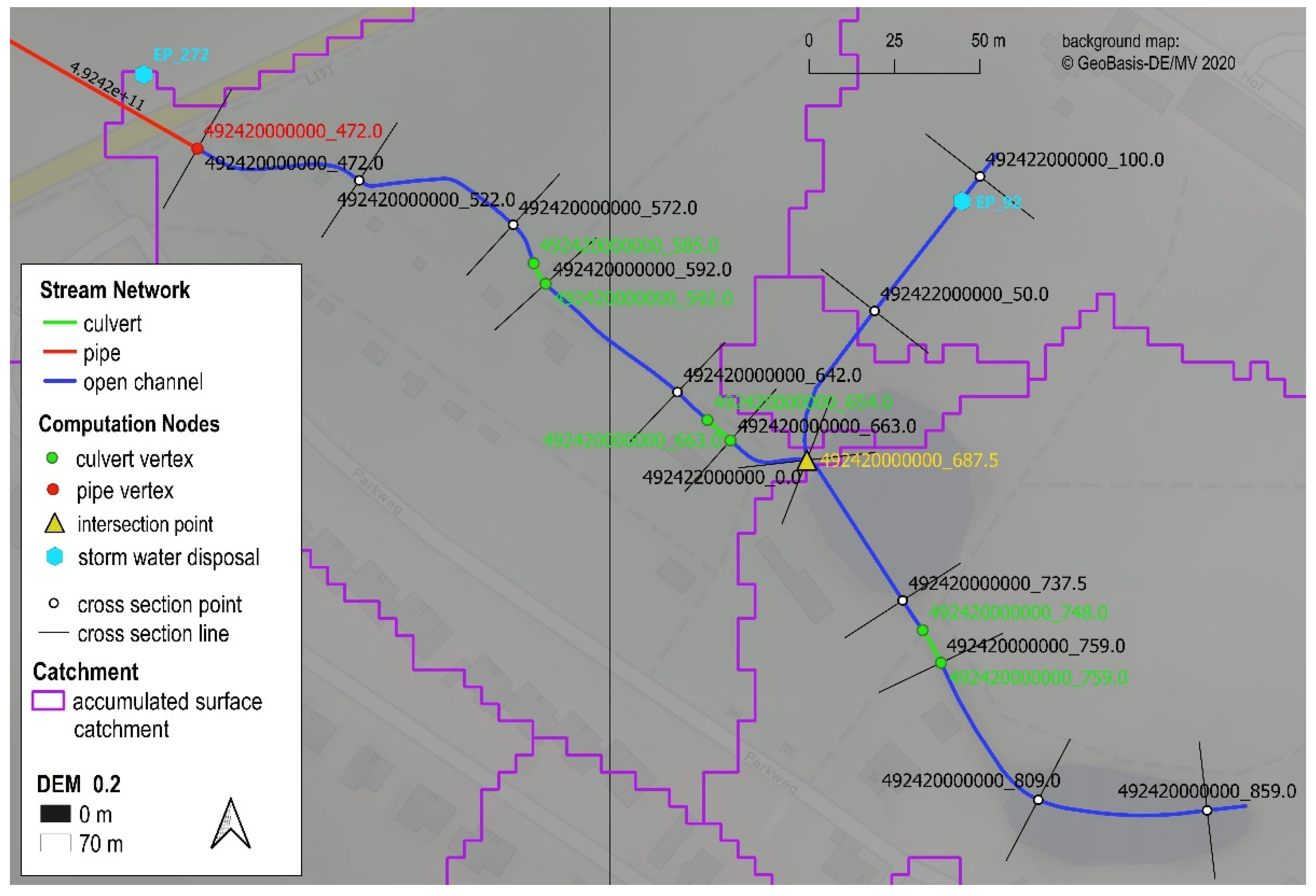
For the construction of the hydrodynamic stream model, mainly vector data in the form of lines are used. These include open channels, pipelines, and culverts (Figure 6). Points are generated at certain positions on these lines, which later become the calculation nodes (or junctions) in SWMM. Cross sections (also called transects in SWMM) of the open channels were generated every 50 m on the basis of the DEM with a cell size of 20 cm. The high spatial resolution thus enables the recording of smaller streams with a width of less than 2 m. When deriving cross profiles using the DEM, it should be noted that the lowest point represents the water level and not the actual invert, if water is present. Since we are interested in flood forecast and thus in high water levels, and the deviation of the absolute water levels in the upper layer of the trapezoidal or parabolic cross-sections is small (<10 cm), this inaccuracy is negligible here.

In addition to the points of the watercourse network, the storm water disposal points are added, which represent the last point of the storm sewer network before the rainwater enters the stream. With the information on the diameter and/or the maximum permissible discharge, the direct runoff from the linked areas can be throttled during the simulation. In this way, the storm sewer network does not have to be included in detail. In the end, five categories of points are produced from which the hydrodynamic model is built: Cross section (open channel), pipe and culvert points, intersection points, and storm water disposal points. They are all assigned a unique ID composed of the hierarchical 12-digit watercourse identification number (WIN) in conjunction with the chainage (e.g., 492000000000_4847.0).

For the rainfall-runoff model, the subcatchments are generated on the basis of the surface subcatchments of the 50 m-stream segments. Since the spatial resolution is quite high, they have to be generalized to save computing time during the simulation. Therefore, the subcatchments of the 50 m-stream segments are accumulated in such a way that new subcatchments start whenever two streams meet or rainwater is discharged from the storm sewer network. Each generated subcatchment is assigned an outlet, which serves to exchange the simulated water volumes between the rainfall-runoff model and the stream. Information on the mean groundwater level is also required for the model construction, which is derived from the groundwater isohypses or from the corresponding interpolated raster map, respectively. The subcatchments are then subdivided according to 13 land use classes (

Table 2. Types of land use in the study area.

Category	Land Use Classes
water	water surface
near natural/ cultivated land	agriculture; wetland; grassland; deciduous forest; mixed forest; coniferous forest; parks; orchard; beach
urban	industry/trade; residential area; traffic area

).

For the intersected subcatchments, mean values of ground height, slope, soil attributes), and degree of sealing are calculated. The point data for the hydrodynamic flow model and the area-based data for the rainfall-runoff model are processed further using Excel and VBA.

2.5. Development of VBA Macros to Automate the Setup of a Combined Hydrological Rainfall-Runoff and a Hydrodynamic Stream Model

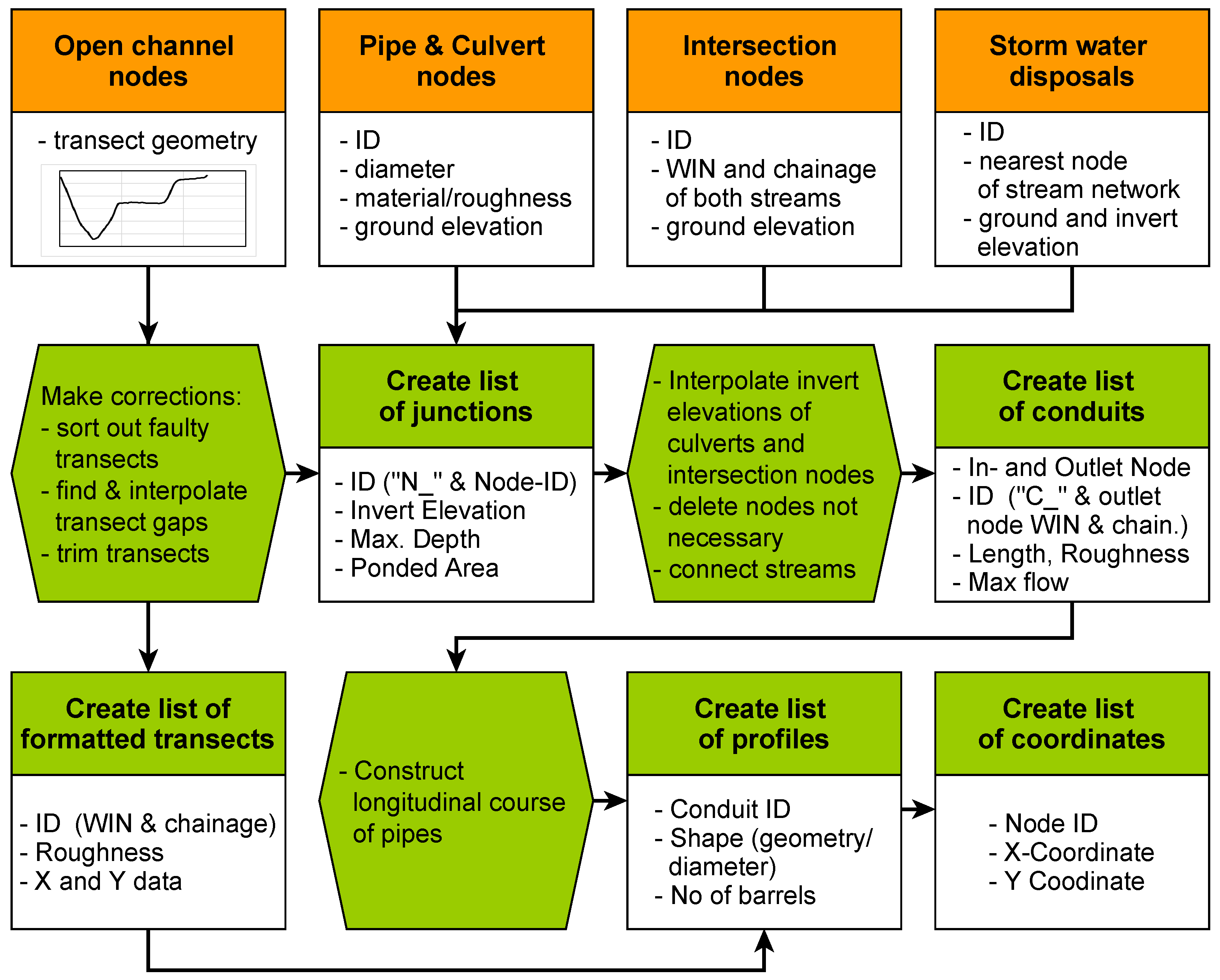
The computation points of the hydrodynamic stream system are loaded into an Excel table and sorted according to their WIN and chainage. After assigning the node properties (Figure 7, attributes = white boxes), the cross sections of the open channels (transects) receive special treatment to a certain extent, as their processing is relatively complex. Once the transect corrections are completed, all categories of calculation points including their attributes can be listed together and sorted in order to create the list of junctions. Now the invert elevations at the culvert and intersection nodes can be interpolated using the open cross-sections upstream and downstream. From the list of junctions, the list of conduits is created. Each conduit is assigned an inlet and outlet node and a unique ID. A flow restriction may only be applied to the conduits connecting the storm water disposals with the stream. If the permitting authorities have specified a diameter for the lower end of the storm sewer channel, then the diameter limits the flow. Otherwise, the flow limitation is realized via the approved peak discharge.

Pipeline routes are designed depending on a specified minimum gradient and a minimum cover with soil, beginning with a depth of 2 m below ground.

For the hydrological rainfall-runoff model, a large part of the work has already been done in QGIS. The output is a large attribute table in which the properties of each subcatchment (surface, land use, soil, and aquifer properties, inlet node of hydraulic network) are stored. The necessary VBA steps now consist of copying the values under the appropriate SWMM headings and formatting them in a software-readable format.

2.6. Model Setup, Calibration, Parameter Transfer and Validation

The catchment and stream model setup was developed and tested in a case study using the Schmarler Bach site. The combined model was consistently built up on the basis of homogenized geodata using VBA macros (VBA—Visual Basic for Applications) to automate the process. By splitting the river course in fairly short sections of about 50 to 100 m, spatially high-resolution flood characteristics (maximum flow, maximum head, maximum capacity, etc.) can be provided for a relatively large area.

After setup, a detailed calibration was performed on the basis of continuous monitoring data of flow and water level. Calibration methods and their fields of application are presented and discussed in [16].

Table 3. Error measures and performance criteria. (taken from [16], supplemented).

Designation	Abbreviated Designation	Formula	No.
Volume error	EVol	$E_{Vol}=1-\frac{{\int }^{\hspace{0.17em}}{Q}_{calc} dt}{{\int }^{\hspace{0.17em}}{Q}_{obs} dt}$	(1)
Mean absolute error	MAE	$MAE=\left|\overline{E}\right|=\frac{{\sum }_t\left|Ob{s}_{i,t}-Cal{c}_{i,t}\right|}{n}$	(2)
Correlation coefficient	R	$R=\frac{{\sum }_t\left(Cal{c}_{i,t}-\overline{Cal{c}_{l,t}}\right)\times \left(Ob{s}_{i,t}-\overline{Ob{s}_{l,t}}\right)}{\sqrt{{\sum }_t{\left(Cal{c}_{i,t}-\overline{Cal{c}_{l,t}}\right)}^2\times {\sum }_t{\left(Ob{s}_{i,t}-\overline{Ob{s}_{l,t}}\right)}^2}}$	(3)
Nash Sutcliffe efficiency	NSE	$NSE=1-\frac{{\sum }_t{\left(Ob{s}_{i,t}-Cal{c}_{i,t}\right)}^2}{{\sum }_t{\left(Ob{s}_{i,t}-\overline{Ob{s}_{l,t}}\right)}^2}$	(4)
Peak error	Epeak	$E_{Peak}=\frac{Q_{calc}}{Q_{obs}}·100$	(5)

Q_calc = calculated flow, Q_obs = observed flow; obs = measured value (observed); calc = calculated value; Indices: i = location, t = time, n = number of measurement data.

presents performance criteria applied to check the model accuracy with regard to the stream flow. It has been supplemented by the peak error E_peak, which represents the relative deviation of the simulated from the observed maximum value of a specific peak flow event.

In the process, physical model parameters were derived from geodata and adjusted to obtain the best model fit regarding stream flow. In a subsequent step, the resulting correlations between geodata and model parameters were transferred to another monitored river basin, the Carbäk catchment, and validated with measured flow data. This way the general validity of the calibrated model parameters is checked, and it is simultaneously tested whether the transfer of largely physically based model parameters is fundamentally satisfactory—despite the different territorial characteristics. After assessing the applicability of this modelling concept, the method was transferred to other river basins in the area without monitoring data.

The parametrized models are finally applied to simulate precipitation scenarios of defined duration and return period in order to generate flood characteristics for the current state of land use. The flood-relevant return period is related to the predominant land uses in the study area and corresponds to the demanded protection level. For heterogeneous land use, this requires defining different return periods and running the model with the appropriate precipitation data.

2.7. Scenario Simulation on the Basis of Defined Rain Events

2.7.1. Selection of Statistical Rainfall Events

When choosing statistical rainfall events, it is first necessary to consider which risk classes are present in the study area. The risk class in turn depends on the predominant land use. For the area of the Hanseatic City of Rostock, assignments of protection levels (return period) to land use classes have already been made (

Table 4. Assignment of land use classes to risk classes (protection level/return period) (excerpt taken from [27], modified).

Protection Level/Return Period	Land Use Class
0 a	Beach Dune Moorland Ruderal land Wooded area	Watercourse > 3 m Ditch < 3 m Standing water body Coastal waters
2 a	Military green space Agricultural grassland
10 a	Arable land Football pitch Tennis court	Sports and recreation Other sports facilities
25 a	Single housing Town square Carpark Allotment	Orchard plantation Rainwater retention basin Campsite
100 a	Row housing Large block housing Sewage treatment plant Railway and railway track	Industry and commerce Motorway Landfill Cemetery

). Within the framework of this study, these were as well transferred to the surrounding rural district.

To determine hydraulic parameters such as statistical flows and water levels as well as profile capacities, simulations were carried out on the basis of statistical precipitation events. Their return periods were selected according to Table 4, whereby a return period of 50 a was additionally taken into account. The duration of the decisive (worst) precipitation event depends primarily on the size of the subcatchment and the corresponding flow length, i.e., the smaller the catchment, the shorter (and at the same time more intense) the decisive rainfall event. Here, the duration categories 1 h, 3 h, 6 h, 9 h, and 12 h were applied and combined with the return periods to generate 18 precipitation scenarios (

Table 5. Selected statistical precipitation events and applied intensity course.

Duration	Return Period	Intensity Course
1 h	2 a, 100 a	statistical calculation according to [28] as described in [29]
3 h	10 a, 25 a, 50 a, 100 a	assumption of a block rain
6 h	10 a, 25 a, 50 a, 100 a	assumption of a block rain
9 h	10 a, 25 a, 50 a, 100 a	assumption of a block rain
12 h	10 a, 25 a, 50 a, 100 a	assumption of a block rain

).

The precipitation amounts were retrieved from the heavy rainfall regionalization (German abbreviation: KOSTRA atlas) of the German Weather Service [30]. The KOSTRA atlas provides raster data on precipitation amounts and intensities per area for Germany as a function of duration D and annuality T (return period). The data are available in an 8.5 km × 8.5 km grid. Each model site is uniformly over-rained, i.e., one representative cell is assigned to each catchment. If a catchment is covered by two or more cells in equal proportions, the cell with the highest precipitation amounts is used.

Since there is usually a clear intensity variation for short durations, the intensity course was statistically determined using the long-term rain data of the monitoring station in Warnemünde (central north of the study area). The data have a temporal resolution of 5 min and were recorded by the German Weather Service. The characteristic precipitation pattern for the respective rainfall duration is obtained by normalising the measured natural rain events of the same duration, which is achieved by temporal centring of the 5 min peak intervals [29].

The application of design rain events in scenario simulation, selected based on stipulated flood reoccurrence intervals, is a pragmatic choice, typically applied in urban hydrology. There is a tendency where the return period of the flood or peak flow is smaller than that of the initializing rainfall event. This way, the choice is “on the safe side”.

2.7.2. Initial Condition

Before the scenario simulations of the different rainfall events can be started, some preliminary work is necessary. Here, the generation of a start condition on which the model rainfall is based is of particular importance. This refers to all reservoir levels in the catchment, i.e., the water level above the terrain, the proportion of the soil pores filled with water, the groundwater level, and the water level in the stream network. For this purpose, the model is run with monthly average evaporation and precipitation data in order to generate a so-called hot start file at the end of the simulation. The final condition of this pre-simulation then forms the start condition for the scenario simulation. In this case, a condition was chosen that leads to average flows in the watercourse.

3. Results and Discussion

3.1. Parameterization

Table 6. Excerpt of important model parameters of the study area (* only SWMM-UrbanEVA).

Parameter	Unit	Value, Range, or Calculation Formula	Subject to Calibration	Spatial Distribution 1,2	Source/Derived from
Surface Runoff
width	m	$\frac{\sqrt{Area}}{6}$	yes	individual	function of area size
percent of impervious area	%	0–94	no	individual	satellite data
average slope	%	0–37	no	individual	DEM
roughness pervious	s/(m1/3)	0.3	yes	pervious area share	in accordance with literature values
roughness impervious	s/(m1/3)	0.025	yes	impervious area share	in accordance with literature values
detention storage pervious	mm	12	yes	pervious area share	in accordance with literature values
detention storage impervious	mm	0.5	yes	impervious area share	in accordance with literature values
Soil infiltration/percolation
max. Infiltration Rate	mm/h	19–281	no	individual	soil maps
min. Infiltration Rate	mm/h	2 −171	no	individual	soil maps
soil porosity	-	0.23–0.79	no	individual	soil maps
field capacity	-	0.1–0.75	no	individual	soil maps
wilting point	-	0.04–0.36	no	individual	soil maps
seepage rate	mm/h	2–171	no	individual	soil maps
Plant parameters *
vegetation factor vf	-	0.7–1.3	yes	land use class dependent	in accordance with literature values
average leaf area index (LAI)	m/m	1.7–3.6	no	land use class dependent	satellite data
LAI monthly coefficients	-	0.2–1.7	no	land use class dependent	satellite data
Groundwater flow
conductivity	mm/h	150	yes	global	in accordance with borehole data and literature values
porosity	-	0.43	yes	global	in accordance with borehole data and literature values
wilting point	-	0.05	yes	global	in accordance with borehole data and literature values
field capacity	-	0.12	yes	global	in accordance with borehole data and literature values
threshold water table elevation	m	1.2 m below ground elevation	yes	global	DEM
lower groundwater loss rate	mm/h	5.0 × 10−6	yes	global	in accordance with borehole data and literature values

¹ individual → each subcatchment has its own individual value; ² global → one value for the entire study area.

presents important model parameters for the dominant processes in the study area. It was the intention to reduce the number of individually calibrated parameters to a minimum and to assign as much as possible parameters directly based on geodata information. In particular, the parameters derived from high spatial resolution geodata, such as the soil maps, were taken as given. For example, infiltration-relevant physical soil properties, such as conductivities, porosity, wilting point, and field capacity, were determined based on the soil type. The most important hydrological processes affecting streamflow are surface runoff, which is responsible for peak flows, and groundwater inflow, which is the base or starting point for peak flows. Therefore, the most effort was put into the calibration of these processes.

Groundwater flow is designed to simulate near-surface agricultural tile drainage. Strictly speaking, it imitates interflow. The threshold water table elevation controls the extent to which water-level groundwater inflow to the stream occurs. It was assumed (or calibrated) that the drainage pipes are on average 1.2 m below ground level. In dealing with the material properties, borehole profiles were surveyed. Many of these contained a near-surface aquifer with an underlying impounding boulder clay layer, which is typical for the northeastern German lowlands. As part of a generalization, the material properties were assumed to be uniform for the entire study area and checked against literature values.

When calibrating surface runoff, the roughness, detention storage, and flow length (=area size/width) play a role. The latter was derived as a function of the area size to ensure parameter transfer. For the former, a distinction was made between sealed and pervious surface portions.

However, soil infiltration and evapotranspiration have an indirect influence on groundwater flow, since they control how much water reaches the groundwater and thus fill the reservoir. Further details can be found in [16].

3.2. Calibration Results

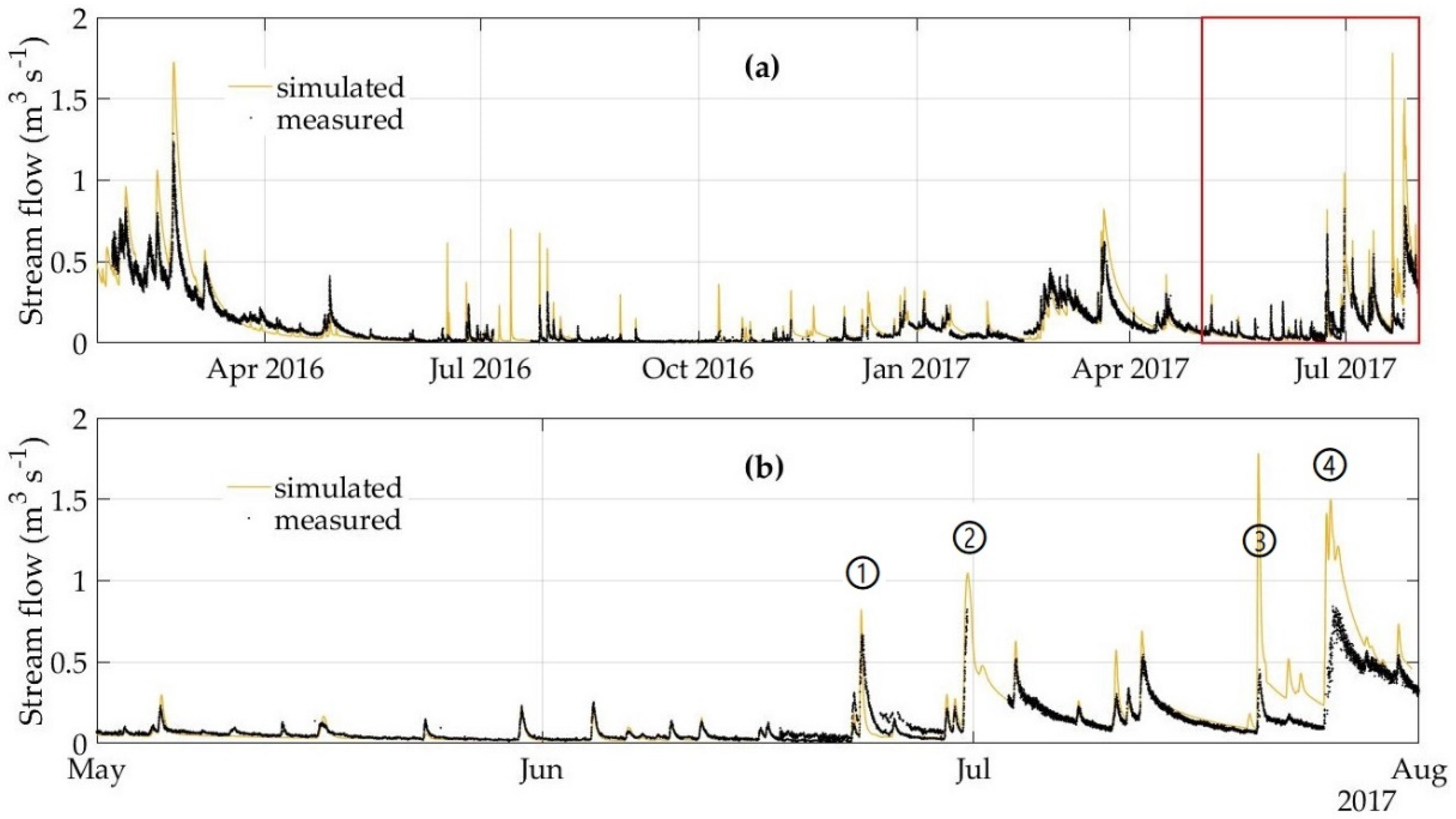
Figure 8 shows the simulated hydrographs with SWMM-UrbanEVA and the corresponding observed stream flows at the monitoring station of the calibration site “Schmarler Bach”. The upper diagram (a) shows the entire observation period (21 January 2016 to 31 July 2017), while the lower diagram (b) focuses on the section from May to July 2017.

Table 7. Model performance based on error measures and performance criteria related to the measured flow rate at the monitoring station in the Schmarler Bach in the period 21 January 2016 to 31 July 2017.

EVol [%]	MAE [m3 s−1]	R [-]	NSE [-]
2.4	0.032	0.84	0.84

presents the corresponding error measures and performance criteria. The visual impression shows a good to very good match between the measured and simulated values. The volume error (E_vol) of 2.4% is very small, as is the mean absolute error (MAE) of 0.03 m³ s⁻¹. The dynamics are well reproduced (correlation coefficient R = 0.84) and the coverage of simulated and measured flows (Nash–Sutcliffe efficiency NSE = 0.84) is overall in the very good range. However, since the focus of this work is primarily on flood characteristics, high flows are of particular interest here. These occur in the catchment area of the Schmarler Bach mainly in the summer months. In particular, the months of June and July 2017 exhibited the highest flows in the observation period. The events of mid/late July even led to local flooding of streets and cellars in the inner city of Rostock [31,32].

While the model apparently reproduces the more frequent, smaller rainfall events very well, there are nevertheless differences between the observed and simulated peak flows for the larger events (Figure 8, diagram b and

Table 8. Peak error of the four largest flows in the observation period at the monitoring station in the Schmarler Bach.

	①	②	③	④
Date	23 June 2017	30 June 2017	20 July 2017	25 July 2017
Peak error (%)	95	110	318	108

). Events 1, 2, and 4 only deviate by a maximum of 10% from those measured, but event 3 (20 July 2017) shows a significant difference as it is more than three times as large as the observed maximum value. Here, it can be assumed that the precipitation centre was directly above the rain gauge (7 km south of the Schmarler Bach) and the catchment itself was located rather on the edge of the rain field at that time. In fact, heavy rainfall events are often short and very localised, especially in urban areas, which was also reflected in the data of different rain gauges in the city of Rostock (cf. Figure 10). The duration of the rain event is considered relatively short (

Table 9. Duration and total amount of corresponding rain events measured at the gauge Uni Rostock Hy.

	①	②	③	④
Date	23 June 2017	30 June 2017	20 July 2017	25 July 2017
Duration of rain event (h)	2.3	17.5	1.3	4.8
Total amount of rain event (mm)	18	41	38	28

) and reinforces the thesis. For this reason, the event of 20 July 2017 is classified as less relevant for the Schmarler Bach.

3.3. Validation Results

Figure 9 shows the simulated hydrographs with SWMM-UrbanEVA and the observed stream flows at the monitoring station of the validation site “Carbäk”.

Table 10. Model performance based on error measures and performance criteria related to the observed flow rate at the monitoring station in the Carbäk stream in the period 27 January 2016 to 17 Aug 2017.

EVol [%]	MAE [m3 s−1]	R [-]	NSE [-]
−9.6	0.045	0.88	0.59

lists the corresponding error measures and performance criteria. While the cumulative flows in the Schmarler Bach are only slightly too low (E_vol = 2.4%), they are 9.6% too high in the Carbäk. The MAE is also higher by 0.013 m³ s⁻¹. However, the dynamics of the flows are reproduced well by the model (R = 0.88). Nevertheless, the individual observed values are less well-met overall compared to the Schmarler Bach. Thus, the Nash–Sutcliffe efficiency coefficient is at the upper (good) edge of the satisfactory range (NSE = 0.59).

Looking more closely at the events of June/July 2017 (Figure 9b;

Table 11. Peak error of the four largest flows in the observation period at the monitoring station in the Carbäk stream.

	①	②	③	④
Date	23 June 2017	30 June 2017	20 July 2017	25 July 2017
Peak error (%)	126	127	394	178

), an overestimation of flows is noticeable here for the extreme events. Events 1 and 2 were overestimated by 26% and 27% respectively, whereby a data gap is to be found for event 2 during the increase in flow. The observed flows therefore probably do not represent the maximum value. As for the Schmarler Bach site, the rainfall event of 20.07.2017 (no. 3) is also classified as not relevant for the Carbäk site. Here, however, it leads to a significant increase in the base flow and thus influences the subsequent event of 25.07.2017 (no. 4).

3.4. Error Discussion

The quality of the results depends to a large extent on the input data. Therefore, important input variables and other possible sources of error are discussed here:

• Input precipitation.

The input precipitation is the crucial input variable and has a decisive influence on the model result. In both cases, Schmarler Bach and Carbäk, the input precipitation was measured outside the model sites, i.e., approximately 7 km south of the Schmarler Bach and 9 km west in the case of the Carbäk, respectively. As mentioned above, there are several precipitation gauges in the study area—but not all of them are set up professionally or they are at least positioned very differently (e.g., on top of a building, underneath a tree, next to a building). Due to the therefore very different systematic measurement error (especially wind error), the measured data are not directly comparable. The only measurement series that is available without gaps in a high temporal resolution (5 min) and could be corrected for the systematic measurement error is the rain gauge “Uni Rostock Hy” of the Department of Hydrology and Applied Meteorology. Therefore, the rain gauge series was applied to the entire study area. However, this does not mean that the measurement series is equally representative for every location in the study area. In particular, heavy rain cells appear in a very localized manner and intensify or weaken significantly along their path. This is exemplified by Figure 10, which illustrates the event on 20 July 2017 (event no. 3) for the different gauges. The gauge “Uni Rostock Hy”, which was used for both model sites, shows the highest measured rainfall intensities, while others closer to the model sites measured less precipitation. Whether this is a consequence of the measurement error cannot be clarified. However, especially against the background of the observed flows, it is very likely that less precipitation actually fell in the two model domains on 20 July.

• Storm water disposals.

With regard to the maximum flows, the throttling via the discharge points plays a significant role. It is possible that not all existing storm water disposals were included in the model setup, but only the officially documented ones. In addition, the diameters of the discharge pipes within the city limits are less well known, so that the throttling was carried out almost exclusively via the approved maximum permissible discharge. In the case that the approved discharge is greater than the actual possible discharge due to existing diameters, it comes to an overestimation of peak flows.

• Size of subcatchments.

Furthermore, the size of the generated subcatchments might affect the resulting maximum flows. A comparison of the two model sites shows that the subcatchments of the Schmarler Bach are, on average, 0.036 km² in size, while the subcatchments of the Carbäk are a little larger (0.051 km² on average). In the case of the Carbäk, the overestimation of runoff peaks of the individual drainage units could be explained by the retention function of small-scale hydrological structures (runoff barriers, small inner basins), which cannot be sufficiently taken into account by the model in large subcatchments.

• Measured flows.

The measured flows themselves can also be subject to errors. Particularly high flows often have to be extrapolated and are usually not verified by comparative multipoint measurements. In the case of the Carbäk monitoring gauge, an ultrasonic doppler flow meter was used to continuously measure the water level and flow velocity in order to calculate the flow rates from the two parameters. Since the device only measures the flow velocity in the central lamella, a calibration function was set up based on regular comparative manual multi-point measurements to obtain the average flow velocity of the complete cross-section. This way, flow rates of up to 0.6 m³ s⁻¹ are confirmed by manual measurements. The highest flows recorded by the continuously measuring device in the timespan June/July 2017 are 0.8 m³ s⁻¹ and thus lie in the extrapolated range of flows. However, since the velocity recorded in the central lamella by the measuring device and the mean profile velocity manually measured have a very strong linear correlation (R = 0.99), the potential error caused by extrapolation is classified as rather small.

3.5. Szenario Simulations Based on Defined Rain Events at the Example of the Schmarler Bach

3.5.1. Initial Condition

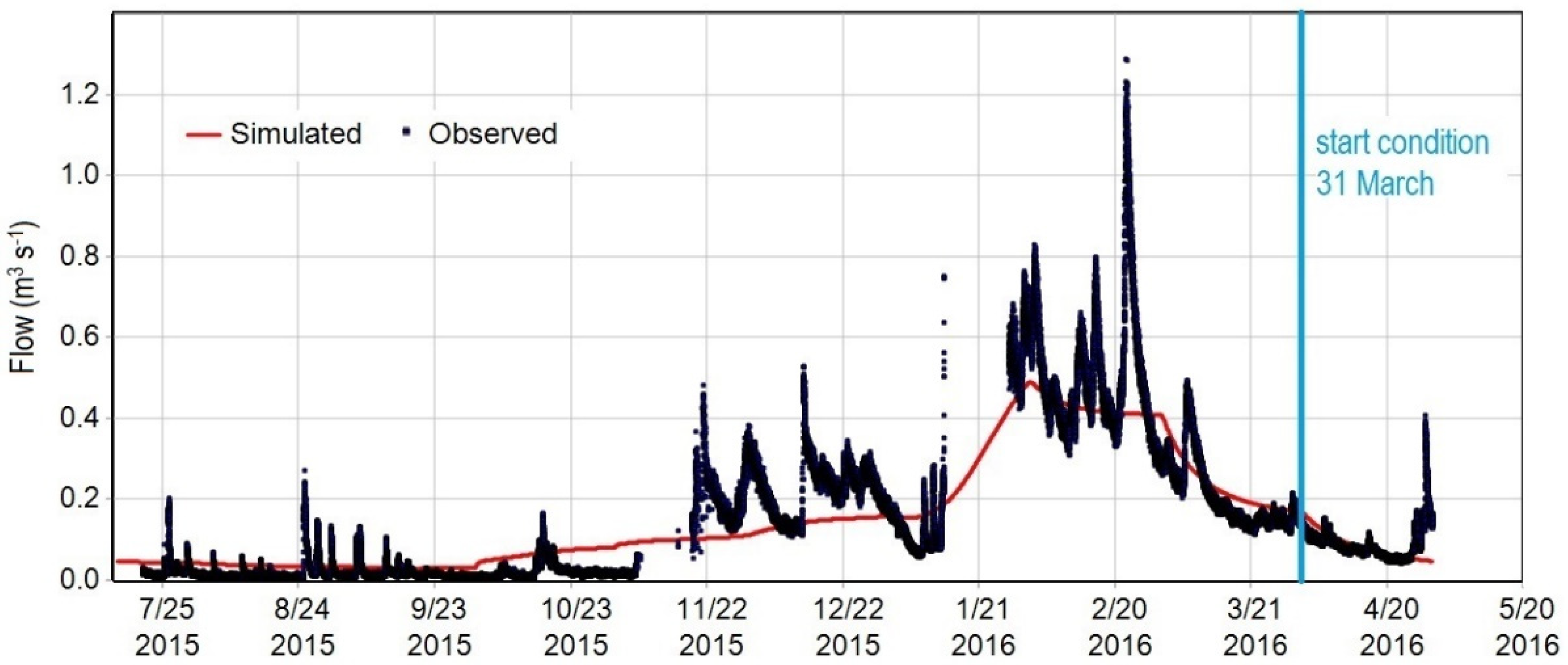
As a starting condition, a state was chosen that leads to average flows in the watercourse. Under the given climatic conditions (highest mean flows in January/February, lowest mean flows in June), such a state arises in March/April, which is why 31 March was chosen as starting point. In order to ensure that a particularly wet or dry month is not picked at random, monthly mean values for the period 2007 to 2017 were calculated for the climate data evaporation and precipitation. The model was initialized with these average data (Figure 11) until the annual course of the flows did not change anymore, which was the case after 2 years. In this way, a hot start file was created for the (average) 31 March, in which the status of all subcatchments, junctions, and conduits is stored. With the hot start file and the introduced model rain, the scenario simulation can now be started.

3.5.2. Intensity Course of Model Rainfall

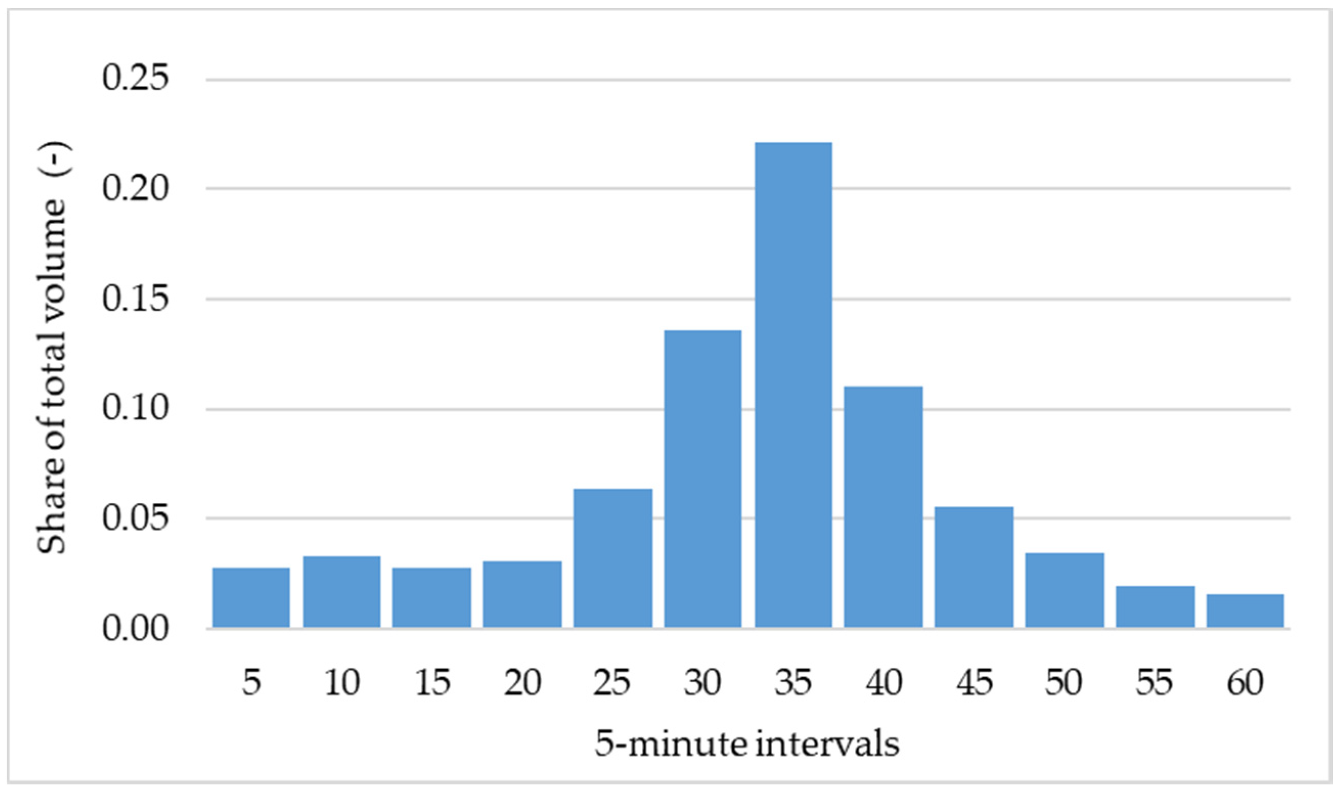
Figure 12 shows the applied intensity course for the 1-h event. The centering of the maximum volume intervals results in a clear intensity course with the highest value during the 35 min interval, in which almost a quarter of the total rain falls. By multiplying the percentages with the total rainfall volume from the KOSTRA atlas, the amount for each interval will be attained.

Since the intensity variability is less prominent for longer durations, a block rain was assumed for the durations ≥ 3 h, i.e., the total amount of precipitation is distributed evenly over the 5-min intervals.

3.5.3. Flood Characteristics for the Current State of Land Use

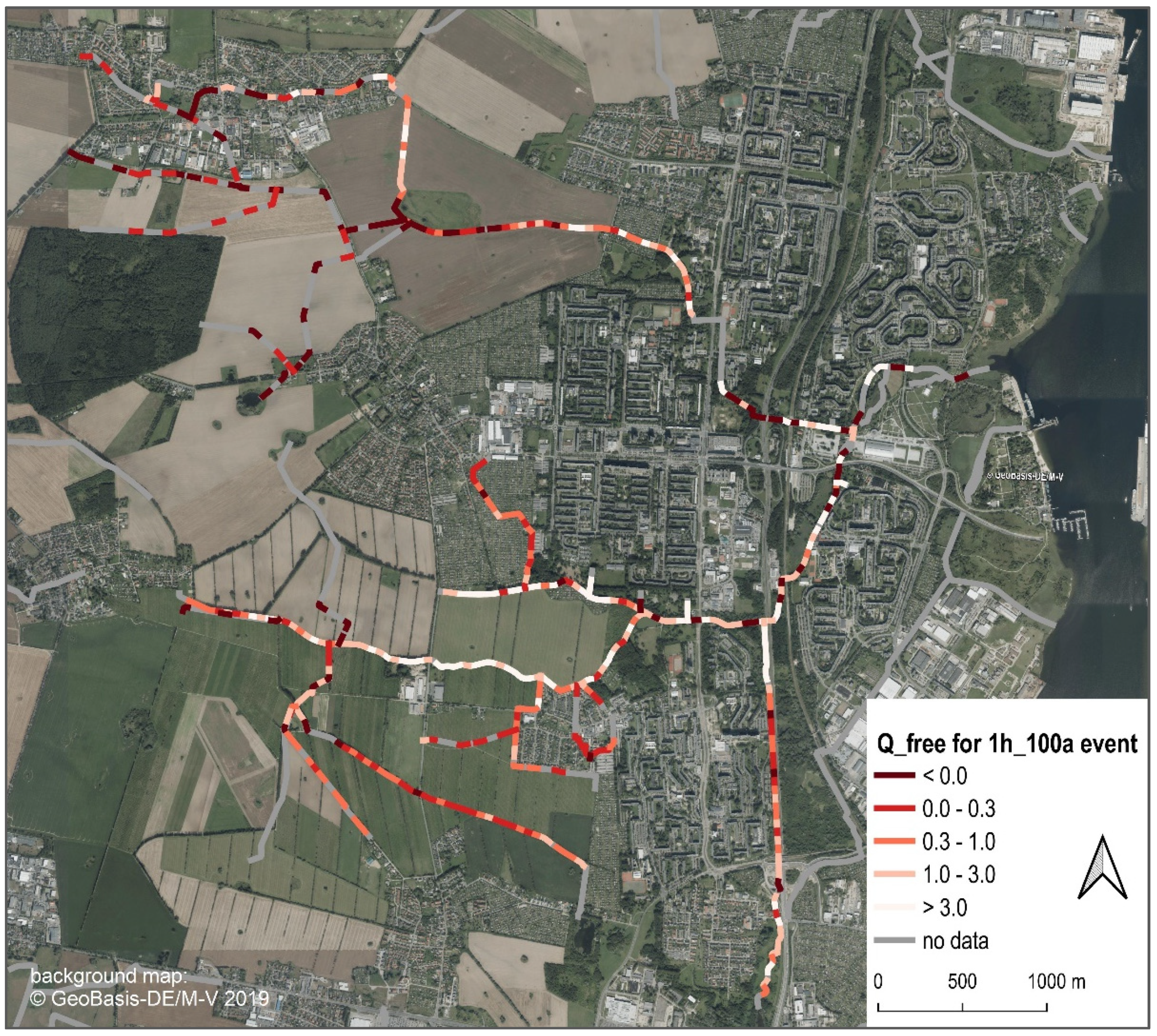
Once the models are set up, they can be used to generate a wide range of results. Some of these are listed in

Table 12. Results from the scenario simulation with defined rainfall events.

		Designation	Unit	Declaration
Watercourses	Conduits	Full_Flow	m3 s−1	Maximum flow at normal flow (water level gradient = bottom gradient)
		max_Flow_rate	m3 s−1	Maximum flow
		max_Flow_velocity	m s−1	Maximum flow velocity
		max_Capacity	-	Proportion of the cross profile filled with water at the time of the maximum water level
		Q_free	m3 s−1	Flow rate that would additionally fit into the cross profile at maximum flow rate; value calculated from model results: Q_free = Full_Flow—max_Flow_rate
	Nodes	max_Hydraulic_head	m above sea level	Maximum absolute Water level
		max_Volume_stored_ ponded	m3	Max. stored volume above banks in case of flooding
		max_Lateral_inflow	m3 s−1	Lateral inflow from the subcatchments
		max_Total_inflow	m3 s−1	Inflow from upstream + lateral inflow from the subcatchments
		max_Flow_lost_flooding	m3 s−1	Excess flow with fully exhausted cross profile; flood volume per unit of time
Subcatchments		max_Runoff_rate	m3 s−1	Maximum direct runoff (surface runoff)
		sum_Runoff_rate	m3	Sum of direct runoff (surface runoff)

. In the context of this work, the focus was primarily on determining the extent to which the watercourses are already at load during defined statistical rainfall events, or how much capacity is still available before flooding sets in. If flooding occurs, it is important to know how much volume will flow out (Table 12 max_Volume_stored_ponded), so that (decentralized) retention measures can be planned if necessary. For the planning of the development of new sites and the associated storm water discharges, these data and information must be available.

Figure 13 illustrates the free capacities in m³ s⁻¹ of the 50 m segments of the Schmarler Bach system at the example of a 1 h rain event with a 100 a return period. Values smaller than zero (dark red) indicate that the segment is already overloaded and overflowing. This is particularly critical when it affects vulnerable land uses and their infrastructural facilities that should not be flooded during a 100-year event, as is the case for example in the northwest of the area. Measures should be introduced here to reduce peak flows. As well, redensification should only be approved if the proportions of the water balance variables are not shifted towards intensification of surface runoff at the expense of infiltration and evaporation.

4. Conclusions and Outlook

The present study shows how robust hydrological/hydraulic models can be set up for small rivers relatively quickly on the basis of geodata and parameter transfer. These can be used to generate spatially highly resolved information of flow and water level for flood risk analysis based on statistical rainfall scenarios.

In the course of parameterization and calibration, the surface runoff and the groundwater interflow turned out to be the most influential processes regarding stream flow. Groundwater parameters, such as conductivities, porosities, etc., were adjusted in the process of calibration and then globally applied to the entire area. A spatially higher resolution would be conceivable, but this would require a very good knowledge of the subsurface layers or involve a complex spatial interpolation. With respect to surface runoff, flow length, roughness, and detention storage in particular were subject to calibration. If the methods were transferred to differing areas, these parameters as well as groundwater parameters would have to be recalibrated. With respect to detention storage, it would also be possible to specify it individually for each subcatchment based on a DEM analysis. This way it would not have been necessary to calibrate the parameter. The average slope, the degree of sealing, and the soil parameters were also derived directly from geodata without calibration. In general, the higher the spatial resolution of the model parameters, the less sense it makes to calibrate individual values of them, since individual small subcatchments sometimes have hardly any visible effect on the results at the observation point. A spatially high model resolution is therefore only recommended with qualitatively good data.

In the study area, the parameter transfer to the validation site only led to a slight loss of model accuracy. Even better model results could have been expected regarding the impact of the suboptimal position of the rain gauge. Provided there is a comparably good geodata situation, the approach offers a good chance to set up fairly reliable models, including hydrodynamic processes, namely for the numerous small rivers without any monitoring.

The construction of river section profiles from laser scanning data introduces a certain error, since only the profile above the water level can be sampled. Still, for small rivers with small water depth, the method seems to be sufficiently exact, since the investigated statistical events create a multiple times higher flow than the flow filling the profile at the scanning date. For larger streams and significant water depth, error compensation strategies could be advisable, like assuming mean flow conditions at the scanning date and subtracting it from the simulated flows to achieve even better results regarding water levels.

For the purpose of flood risk analyses, the main advantages compared to a simple GIS-based flood regionalization are (i) the physically integrated and highly distributed land use and (ii) the inclusion of stream hydrodynamics. This way, even small-scale land-use changes can be directly incorporated and analyzed. The hydrodynamic functionality not only provides water level but can also be used in targeted development of the river system and its infrastructures.

With its extension UrbanEVA, SWMM also provides the functionality of a full water balance model. Accordingly, the model can be used as well to quantify alterations in the water balance for planned land use changes, particularly the surface runoff that potentially triggers flooding. Recently, the new mandatory German standard DWA-A 102-1 [33] requires that spatial planning must not fundamentally change the quantitative proportions of water balance variables. This will lead to a significant boost for low-impact design (LID) in urban areas. Initially, SWMM-UrbanEVA was exactly developed for the purpose of better describing LID structures in urban hydrology. In our study, detailed urban drainage infrastructure is purposely not included, but the model environment would allow for such refining.

References

1. Zhou, T.; Endreny, T. The Straightening of a River Meander Leads to Extensive Losses in Flow Complexity and Ecosystem Services. Water 2020, 12, 1680. [Google Scholar] [CrossRef]
2. Park, G.; Park, H. Influence analysis of land use by population growth on urban flood risk using system dynamics using system dynamics. In Environmental Impact IV; Environmental Impact 2018, Naples, Italy, 6/20/2018–6/22/2018; Casares, J., Passerini, G., Perillo, G., Eds.; WIT Press: Southampton, UK, 2018; pp. 195–205. [Google Scholar]
3. Handayani, W.; Chigbu, U.E.; Rudiarto, I.; Putri, I.H.S. Urbanization and Increasing Flood Risk in the Northern Coast of Central Java—Indonesia: An Assessment towards Better Land Use Policy and Flood Management. Land 2020, 9, 343. [Google Scholar] [CrossRef]
4. Poelmans, L.; van Rompaey, A.; Batelaan, O. Coupling urban expansion models and hydrological models: How important are spatial patterns? Land Use Policy 2010, 27, 965–975. [Google Scholar] [CrossRef]
5. Ungaro, F.; Calzolari, C.; Pistocchi, A.; Malucelli, F. Modelling the impact of increasing soil sealing on runoff coefficients at regional scale: A hydropedological approach. J. Hydrol. Hydromech. 2014, 62, 33–42. [Google Scholar] [CrossRef] [Green Version]
6. Alexakis, D.D.; Grillakis, M.G.; Koutroulis, A.G.; Agapiou, A.; Themistocleous, K.; Tsanis, I.K.; Michaelides, S.; Pashiardis, S.; Demetriou, C.; Aristeidou, K.; et al. GIS and remote sensing techniques for the assessment of land use change impact on flood hydrology: The case study of Yialias basin in Cyprus. Nat. Hazards Earth Syst. Sci. 2014, 14, 413–426. [Google Scholar] [CrossRef] [Green Version]
7. Semadeni-Davies, A.; Hernebring, C.; Svensson, G.; Gustafsson, L.-G. The impacts of climate change and urbanisation on drainage in Helsingborg, Sweden: Combined sewer system. J. Hydrol. 2008, 350, 100–113. [Google Scholar] [CrossRef]
8. Miller, J.D.; Hutchins, M. The impacts of urbanisation and climate change on urban flooding and urban water quality: A review of the evidence concerning the United Kingdom. J. Hydrol. Reg. Stud. 2017, 12, 345–362. [Google Scholar] [CrossRef] [Green Version]
9. U.S. Geological Survey. The 100-Year Flood. Available online: https://www.usgs.gov/special-topic/water-science-school/science/100-year-flood?qt-science_center_objects=0#qt-science_center_objects (accessed on 28 June 2021).
10. Seibert, J. Regionalisation of parameters for a conceptual rainfall-runoff model. Agric. Forest Meteorol. 1999, 98–99, 279–293. [Google Scholar] [CrossRef]
11. Song, J.-H.; Her, Y.; Suh, K.; Kang, M.-S.; Kim, H. Regionalization of a Rainfall-Runoff Model: Limitations and Potentials. Water 2019, 11, 2257. [Google Scholar] [CrossRef] [Green Version]
12. Servat, E.; Dezetter, A. Rainfall-runoff modelling and water resources assessment in northwestern Ivory Coast. Tentative extension to ungauged catchments. J. Hydrol. 1993, 148, 231–248. [Google Scholar] [CrossRef]
13. Ibrahim, A.B.; Cordery, I. Estimation of recharge and runoff volumes from ungauged catchments in eastern Australia. Hydrol. Sci. J. 1995, 40, 499–515. [Google Scholar] [CrossRef]
14. Garambois, P.A.; Roux, H.; Larnier, K.; Labat, D.; Dartus, D. Parameter regionalization for a process-oriented distributed model dedicated to flash floods. J. Hydrol. 2015, 525, 383–399. [Google Scholar] [CrossRef] [Green Version]
15. Tränckner, J.; Walter, A.; Bill, R.; Richter, B.; Hoche, H.; Hoffmann, T.; Jungnickl, C.; Kachholz, F.; Mehl, D.; Schmeil, S.; et al. KOGGE: Kommunale Gewässer gemeinschaftlich entwickeln: Ein Handlungskonzept für kleine urbane Gewässer am Beispiel der Hanse- und Universitätsstadt Rostock; Universität Rostock, Professur für Wasserwirtschaft, Agrar- und Umweltwissenschaftliche Fakultät: Rostock, Germany, 2018; ISBN 978-3-86009-476-1. [Google Scholar]
16. Kachholz, F.; Tränckner, J. Long-Term Modelling of an Agricultural and Urban River Catchment with SWMM Upgraded by the Evapotranspiration Model UrbanEVA. Water 2020, 12, 3089. [Google Scholar] [CrossRef]
17. QGIS.org. QGIS User Guide: Release 2.18. Available online: https://docs.qgis.org/2.18/pdf/en/QGIS-2.18-UserGuide-en.pdf (accessed on 9 April 2021).
18. QGIS.org. QGIS Geographic Information System. QGIS Association. 2021. Available online: http://www.qgis.org (accessed on 5 May 2021).
19. Microsoft Corporation. Microsoft Excel; Microsoft Ireland Operations Limited: Dublin, Ireland, 2019. [Google Scholar]
20. The Document Foundation. LibreOffice Calc; The Document Foundation: Berlin, Germany, 2020. [Google Scholar]
21. Waseem, M.; Kachholz, F.; Tränckner, J. Suitability of common models to estimate hydrology and diffuse water pollution in North-eastern German lowland catchments with intensive agricultural land use. Front. Agr. Sci. Eng. 2018. [Google Scholar] [CrossRef] [Green Version]
22. US Army Corps of Engineers—Hydrologic Engineering Center. HEC-HMS (Hydrologic Modeling System); US Army Corps of Engineers—Hydrologic Engineering Center: Davis, CA, USA, 2021.
23. US Army Corps of Engineers—Hydrologic Engineering Center. HEC-RAS (River Analysis System); US Army Corps of Engineers—Hydrologic Engineering Center: Davis, CA, USA, 2021. [Google Scholar]
24. Hörnschemeyer, B.; Henrichs, M.; Uhl, M. SWMM-UrbanEVA: A Model for the Evapotranspiration of Urban Vegetation. Water 2021, 13, 243. [Google Scholar] [CrossRef]
25. U.S. EPA. Storm Water Management Model (SWMM); U.S. EPA—United States Environmental Protection Agency: Durham, NC, USA, 2020.
26. Rossman, L. Storm Water Management Model: User’s Manual Version 5.1. EPA/600/R-14/413 (NTIS EPA/600/R-14/413b). Available online: https://www.epa.gov/sites/production/files/2019-02/documents/epaswmm5_1_manual_master_8-2-15.pdf (accessed on 23 June 2021).
27. Mehl, D.; Hoffmann, T.; Schneider, M.; Lange, A.; Foy, T. Integraler Entwässerungsleitplan (IELP) für die Hansestadt Rostock: Definition von Hauptentwässerungsachsen (HEA). Available online: https://rathaus.rostock.de/media/rostock_01.a.4984.de/datei/Endbericht_IELP_20161108.pdf (accessed on 29 April 2021).
28. Otter, J.; Königer, W. Bemessungsregen für Kanalnetz, Regenüberläufe und Regenbecken. Gas-Wasser-Abwasser 1986, 66, 124–128. [Google Scholar]
29. DWA. Arbeitsblatt DWA-A 118. Hydraulische Bemessung und Nachweis von Entwässerungssystemen; März 2006; DWA: Hennef, Germany, 2006; ISBN 3939057150. [Google Scholar]
30. Junghänel, T.; Ertel, H.; Deutschländer, T. KOSTRA-DWD-2010R Deutscher Wetterdienst: Bericht zur Revision der Koordinierten Starkregenregionalisierung und -Auswertung des Deutschen Wetterdienstes in der Version 2010. Offenbach am Main. 2017. Available online: https://www.dwd.de/DE/leistungen/kostra_dwd_rasterwerte/download/bericht_revision_kostra_dwd_2010.pdf?__blob=publicationFile&v=6 (accessed on 7 July 2021).
31. Schmidtbauer, B. Starkregen verschärft Gefahren an den Steilküsten in MV. Ostsee-Zeitung. 4 January 2018. Available online: https://www.ostsee-zeitung.de/Nachrichten/MV-aktuell/Starkregen-verschaerft-Gefahren-an-den-Steilkuesten-in-MV (accessed on 20 April 2021).
32. Tretropp, S. Unwetter in Rostock: Straßen gesperrt, Keller voll, Autos abgesoffen. svz.de. 20 July 2017. Available online: https://www.svz.de/lokales/rostock/strassen-gesperrt-keller-voll-autos-abgesoffen-id17360741.html (accessed on 20 April 2021).
33. DWA-Arbeitsgruppe ES-2 1. und BWK_Arbeitsgruppe 2. Arbeitsblatt DWA-A 102-1/BWK-A 3-1 Grundsätze zur Bewirtschaftung und Behandlung von Regenwetterabflüssen zur Einleitung in Oberflächengewässer—Teil 1: Allgemeines; Dezember 2020; Deutsche Vereinigung für Wasserwirtschaft, Abwasser und Abfall: Hennef, Germany, 2020; ISBN 9783968620459. [Google Scholar]
Figure 1. Relevant surface catchments of the study area, administrative boundaries, and rain gauge used for simulations.
Hydrology 08 00102 g001
Figure 2. Schmarler Bach catchment used for model calibration.
Hydrology 08 00102 g002
Figure 3. Carbäk stream catchment used for model validation.
Hydrology 08 00102 g003
Figure 4. Measured flow at the two monitoring stations in the Schmarler Bach and in the Carbäk; measured precipitation approximately 7 km south of the Schmarler Bach catchment and 9 km west of the Carbäk, respectively.
Hydrology 08 00102 g004
Figure 5. Pre-processing of flood characteristics for the current state of land use (orange: QGIS tools, green: VBA and MS Excel tools, blue: SWMM-UrbanEVA, light blue: SWMM).
Hydrology 08 00102 g005
Figure 6. Calculation nodes of the stream network composed of pipe and culvert vertices, cross sections points, intersection points, and storm water disposals (DEM_0.2 = digital elevation model with a cell size of 0.2 m).
Hydrology 08 00102 g006
Figure 7. Hydraulic flow model build-up—steps to create the SWMM-input file (orange: QGIS output; green: VBA/Excel steps; white boxes contain respective attributes).
Hydrology 08 00102 g007
Figure 8. Comparison of simulated and measured flows at the monitoring station (chainage 2+417) of the Schmarler Bach (calibration site); the red box in the upper (a) diagram marks the time span of the lower (b) diagram.
Hydrology 08 00102 g008
Figure 9. Comparison of simulated and measured flows at the monitoring station (chainage 3+413) of the Carbäk stream (validation site); the red box in the upper (a) diagram marks the time span of the lower (b) diagram.
Hydrology 08 00102 g009
Figure 10. Different rain gauges of the study area and measured rainfall on 20 July 2017 (green catchment: Schmarler Bach, purple catchment: Carbäk).
Hydrology 08 00102 g010
Figure 11. Comparison of the simulated flows (m3 s−1) based on monthly average evaporation and precipitation data and the observed flows using the example of the Carbäk stream.
Hydrology 08 00102 g011
Figure 12. Statistically derived intensity course of the 1 h-rain event.
Hydrology 08 00102 g012
Figure 13. Q_free—Flow rate (m3 s−1) that would additionally fit into the cross profile at maximum flow rate regarding a rainfall event of 1 h duration and 100 a return period.
Hydrology 08 00102 g013