Article

Assessment of the Impact of Climate Change on Snow Distribution and River Flows in a Snow-Dominated Mountainous Watershed in the Western Hindukush–Himalaya, Afghanistan

by
Abdul Haseeb Azizi
1,2 and
Yoshihiro Asaoka
3,*
1
Department of Civil Engineering, Graduate School of Engineering, Nihon University, Koriyama 963-8642, Japan
2
Department of Floods, Droughts and Climate Change Predictions, Directorate General of Water Resources, National Water Affairs Regulation Authority, Kabul 1004, Afghanistan
3
Department of Civil Engineering, College of Engineering, Nihon University, Koriyama 963-8642, Japan
*
Author to whom correspondence should be addressed.
Hydrology 2020, 7(4), 74; https://doi.org/10.3390/hydrology7040074
Submission received: 10 September 2020 / Revised: 1 October 2020 / Accepted: 4 October 2020 / Published: 6 October 2020
(This article belongs to the Special Issue Climate Change Effects on Water Resources Management)

Abstract

:
Projected snow cover and river flows are important for planning and managing water resources in snow-dominated basins of the Himalayas. To quantify the impacts of climate change in the data scarce Panjshir River basin of Afghanistan, this study simulated present and future snow cover area (SCA) distributions with the snow model (SM), and river flows with the snowmelt runoff model (SRM). The SRM used the degree-day factor and precipitation gradient optimized by the SM to simulate river flows. Temperature and precipitation data from eight kinds of general circulation models (GCMs) were used for bias correction. The SM and SRM were first calibrated and validated using 2009–2015 data, and then bias-corrected future climate data were input to the models to simulate future SCA and river flows. Under both the representative concentration pathways (RCP) 4.5 and 8.5, the annual average SCA and river flow were projected to decrease in the mid and late 21st century, although seasonal increases were simulated in some instances. Uncertainty ranges in projected SCA and river flow under RCP 8.5 were small in the mid 21st century and large in the late 21st century. Therefore, climate change is projected to alter high-altitude stream sources in the Hindukush mountains and reduce the amount of water reaching downstream areas.

1. Introduction

Climate change is expected to alter the hydrological cycle and influence both water availability and demand [1]. Because the effects of climate change on water resources are complex and ambiguous, adaptation to the changing climate is a major challenge in the world today. Climatic variability is much greater in the Hindukush–Himalaya (HKH) mountainous region of Afghanistan, Bangladesh, Bhutan, China, India, Myanmar, Nepal, and Pakistan, than in other parts of the world [2,3]. Glaciers are one of the most important indicators of climate change [4,5], and the HKH region is host to some of the world’s largest glaciers [6,7,8], which are the major water source of the Indus, Brahmaputra, and Ganges rivers [9,10]. These river basins are extremely sensitive to both spatial and temporal changes in climate [3]. HKH glaciers are among the fastest thinning glaciers in the world [11]. The temperature is projected to increase in the HKH region by 1.7 °C to 6.3 °C by the end of the 21st century [12]. In many parts of the HKH region, monsoonal precipitation is projected to increase, and extreme precipitation events are projected to become more frequent [12,13], although in the western HKH region, precipitation declines are more probable [12,13,14,15].
Through effects such as more rapid melting of snow and ice and an increased incidence of natural hazards, rising temperatures will directly affect human society, especially in mountainous environments. In addition, increases in the intensity and frequency of extreme precipitation events are expected to result in higher surface flow rates and increased flood risks [16]. Moreover, climate change will lead to more variability in the hydrological cycle [14], including more frequent floods and droughts with higher intensities, which will increase erosion, sedimentation, and water scarcity. Furthermore, losses of glaciers, sea ice, and snow cover, disruptions to water quality, and the degradation of ecosystems are expected to become more extreme in the future as a consequence of these impacts of climate change on the hydrological cycle and water resources [17]. Rising temperatures will also cause snow and glacier covered areas to decline as a result of both increased melting of the snow and ice pack and lower snow accumulation due to less precipitation falling as snow [18]. Hence, climate change and climate variability are likely to influence the availability of water in mountain basins and, in the long term, adversely affect the livelihood of people, in particular, those living in downstream areas.
Snow and ice meltwaters play a significant role throughout the HKH region because they provide water for downstream farming, generating hydropower, and domestic use [19]. The HKH region is estimated to contribute 50–80% of the snow and glacier meltwaters received by the Indus River basin [19,20,21,22,23]. However, upstream snow and ice reserves in the HKH region, particularly in the Brahmaputra and Indus River basins, are expected to be affected by climate change, and the resulting changes in the volume, intensity, and spatial distribution of meltwaters will threaten the water availability and food security of a large number of people [24]. Because of high climate variability, data scarcity, large uncertainties in projected climate changes, and ambiguity respecting the response of glaciers, the study of climate change impacts on the hydrology of glacier covered high-altitude catchments in the Himalayas is challenging [25]. In mid-latitude mountainous regions, the changing climate has had major impacts on snow cover. In particular, climate change has led to spatial and temporal variations in both snow cover and meltwater runoff [26]. Increased water demand due to the expected socio-economic growth and rising populations means that climate variability is likely to place an even greater strain on water resources [27]. Thus, to identify the impacts of past, present, and future climate change on mountain river basins, a better understanding of the impacts of climate change on mountain hydrological cycles is needed [27].
Previous climate variability studies in the HKH region, conducted at both large and small scale, have concluded that climate change will likely impact river flows that are driven by snow and glacier melt. Immerzeel et al. [25] have reported that in the Langtang basin in Nepal, temperature and precipitation can be expected to increase by 0.06 °C/year and 1.9 mm/year, respectively. They estimated that, under climate change, glaciers will decline 32% by 2035, 50% by 2055, and 75% by 2088. Shrestha and Nepal [6] assessed the effects of climate change on the water balance in the Hunza catchment, a sub-basin of the Indus River basin, and estimated that future discharge of the Hunza River would decrease by 28%, 40%, and 46% under scenarios in which glaciers receded to 4000, 4500, and 5000 m above mean sea level (a.m.s.l.). Hayat et al. [28], who studied both present and future runoff by using a snowmelt runoff model and Representative Concentration Pathway (RCP) scenarios, showed that the mean annual runoff in the Astore and Hunza watersheds in Pakistan will probably increase by 11% to 58% by the mid-21st century, and by 14% to 90% by the late 21st century.
Physically based energy-balance models are essential for understanding snowmelt processes [29]. However, this group of models needs more input data [30] and therefore have limited applicability in data-scarce basins. On the other hand, temperature index algorithms are used widely for the water resources assessment in the sparsely gauged snow-fed large basins. Studies that have assessed the ability of the snowmelt runoff model (SRM) [31] in the data scarce HKH and Tibetan Plateau regions have found that the model performed well for river flow simulations [18,20,32,33,34,35,36]. Other studies have used the SRM to investigate how future increases or decreases in temperature and precipitation rate would affect river flows [26,37,38,39,40,41].
The impacts of climate change on the HKH region have also been evaluated by integrating general circulation models (GCMs) or regional circulation models with the SRM to simulate future water availability in mountainous basins [28,42,43,44,45]. Required input climate variables to the SRM include daily temperature, daily precipitation, and daily snow-covered area [31], but most past studies have focused on the impacts of temperature and precipitation on climate variability, considering the snow-covered area only hypothetically in future runoff simulations. One of the major sources of uncertainty in these studies is the use of assumed future snow-covered area values to simulate the future meltwater discharge from the mountain snowpack and glaciers. Therefore, it is necessary to simulate the future snow cover area distribution especially in snow-dominated basins under various climate change scenarios.
In the present study, before simulating runoff with the SRM, in the first step, the Snow Model (SM) was used [46] to estimate the future snow cover area distribution under different RCP scenarios. The SM has the ability to model the spatial and temporal distribution of snowfall, the snow-covered area, snowmelt rate, and the snow water equivalent (SWE) of the snowpack [46,47,48,49,50]. In the Hindukush region, to the best of our knowledge, no study has yet been conducted to quantify snow characteristics and melt runoff during present and future periods. Therefore, the specific objectives of this study were (1) to assess the impact of future climate changes on the snow-covered area and streamflow under different climate change scenarios, and (2) to evaluate uncertainties in the climate model projections.

2. Study Area

Our study area was the Kabul River basin in northeast Afghanistan. The Kabul River originates in the Hindukush mountains and is a tributary of the Indus River (Figure 1). The Kabul River basin has an area of about 87,615 km2 and ranges in elevation from 400 m to 7603 m a.s.l. [15]. The basin climate is semi-arid and strongly continental. The northern and northeastern parts of the basin are characterized by complex topography and high mountain peaks with high-elevation areas dominated by snow and glaciers. In the southern and eastern parts of the basin, precipitation is low, whereas it is high in the northern and northeastern parts. The average annual air temperature is about 22 °C in eastern downstream locations, but approximately 14 °C in central upstream locations. The maximum and minimum temperatures in the basin are observed in July and January, respectively.
Annual average precipitation in the northern and north-eastern central parts of the basin is 450 mm, but only 300 mm in the south and eastern downstream parts. Nearly all precipitation falls as snow during the winter, and it is stored throughout the mountains to recharge the rivers in the melt season. Approximately 1274 glaciers, with a total area of 1594 km2 and estimated ice reserves of 177 km3, have been mapped in the Kabul basin [51]. The Kabul River flows eastward through Afghanistan and Kabul, and then, after entering Pakistan, it joins the Indus River east of Peshawar. It is fed by several small and large tributary rivers that originate in high-altitude areas of the basin. The main tributaries are the Logar, Panjshir (and its own major tributary, the Ghorband River), Laghman, and Kunar rivers. The Kabul basin occupies 12% of Afghanistan’s national territory, but it accounts for one-fourth (26%) of the country’s total annual water flow [52,53]. The river feeds over 300,000 ha of intensively irrigated fields supporting high-value crops in Afghanistan [53]. Climate change is expected to adversely affect the irrigated areas of the Kabul basin mainly through extreme weather events, such as droughts and floods [54].
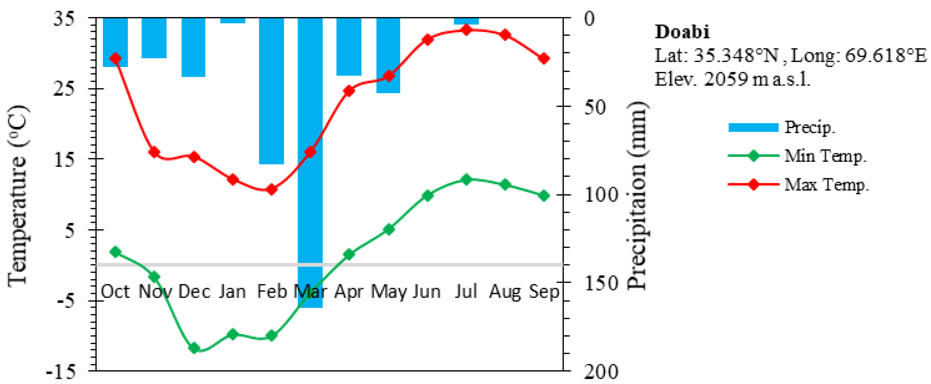
This study was focused on the Panjshir sub-basin of the Kabul basin (Figure 1). The sub-basin covers an area of about 3540 km2, as calculated by using the Advanced Spaceborne Thermal Emission and Reflection Radiometer (ASTER) Global Digital Elevation Model (GDEM) product [55]. Its mean elevation is approximately 3498 m a.s.l., as calculated from the hypsometric curve, and its maximum elevation is around 5694 m a.s.l. (Figure 2). The Panjshir River originates in the high mountainous region of the Hindukush characterized by seasonal snow cover and glaciers, and it joins the Kabul River below its confluence with the Ghorband River on the Shamali Plain. Annual discharge from the Panjshir sub-basin, including the Ghorband sub-basin, to the Kabul River is second largest, after the Kunar River. In the Panjshir sub-basin, maximum precipitation is observed during the winter months (February and March), and the mean total annual precipitation measured at Doabi climate station is about 336 mm. The maximum summertime temperature is observed in July (average, 24 °C), and the average minimum wintertime temperature is approximately –17 °C (Figure 3). Because of the intricate terrain, there is a large spatial variation in the amount of precipitation over the course of a year. The climatic conditions of the Panjshir sub-basin generally allow one crop to be grown each year with occasional crop rotation [56]. The estimated mean annual actual evapotranspiration is about 450 mm [57].

3. Materials and Methods

3.1. Datasets

The ASTER GDEM product with a 30 m spatial resolution was utilized to create a hypsometric curve of the study area (Figure 2), to delineate the study catchment area, and to assess topographical features such as altitudinal zones and their areas.
Daily climatic data (air temperature and precipitation) observed at hydro-meteorological stations in the study area were obtained from the Water Resources Department (WRD)/Ministry of Energy and Water-Afghanistan (MEW-A) for the period from 2009 to 2015. Further, daily discharge measured from 2009 to 2015 at the basin outlet was also acquired from WRD/MEW-A (Table 1). There are six hydro-meteorological stations in Panjshir sub-basin. Air temperature and precipitation data from all of these stations were used on a daily basis. Location of these hydro-meteorological stations are presented in Figure 1.
Remotely sensed snow cover data were derived from the Moderate Resolution Imaging Spectroradiometer (MODIS) snow cover product, which provides the snow-covered area with a spatial resolution of nearly 500 m. This study uses the combined data acquired at 8-day intervals by Terra (MOD10A2) and Aqua (MYD10A2) sensors for the entire HKH region [58] (i.e., the maximum snow-covered area observed during each 8-day period [59]). The approach used for obtaining the SCA maps from MODIS images takes advantage of the binary snow cover data of product V5 [58]. The MODIS snow cover product has been widely used for simulations of river discharge [20,43,60,61,62].
To assess future changes in temperature and precipitation, eight Coupled Model Inter-comparison Project Phase 5 (CMIP5) general circulation models (GCMs) were used (Table 2). In the present study, two RCP scenarios are considered: 4.5 and 8.5 for future climate projections.

3.2. Methods

In this study, we first applied the Snow Model (SM) which has previously been investigated for the Panjshir sub-basin [46] to evaluate the impact of future climate changes on the snow-covered area. SM was used to optimize the degree-day factor (DDF) and precipitation gradient (PG) using satellite data and finally, it simulated the daily snow-covered area (SCA) [46]. The SM developed for the Panjshir sub-basin adopts a different approach from SnowModel developed by Liston and Elder [63]. SnowModel is a physically based energy-balance model [63]. SnowModel needs extensive meteorological data, as well as calculating individual snow layer settlement [64]. Although, because of its strong data and computational requirements, this appears to be difficult to apply to large basins and areas [64]. The SM developed for Panjshir sub-basin is a degree-day-based model that can efficiently simulate the spatiotemporal distribution of snowfall, the snow-covered area, the snowmelt rate, and the SWE of the snowpack [46,47]. The major benefits of this approach are its simplicity, large availability of air temperature data and the calculation performance in calibration and simulation [65,66]. SM estimates the distribution of snowfall, snow covered area, snowmelt and SWE for each grid cell. The grid cell size is about 30 m which is based on the ASTER GDEM for the present study.
To simulate temporal variations in the SWE, the following equation is used:
SWEt+1 = SWEt + (SFt − SMrt) dt
where SWE is snow water equivalent (mm), SF is the daily snowfall in each pixel (mm d–1), SMr is the daily snowmelt rate (mm d–1), the subscript t represents the date, and dt is one day. The daily snowmelt rate is estimated by the degree-day method:
SMrt = DDF × Tat
where SMr is the daily snowmelt rate (mm d–1), DDF is the degree-day factor (cm °C–1 d–1), and Ta is the daily mean air temperature (°C). The base temperature, below which no snowmelt is considered to occur, is 0 °C [49,50,67]. Daily precipitation at the measurement stations was estimated to a grid by interpolation:
P = (1 + PG (h − elvobs)) Pobs
where P is daily precipitation (mm d–1) at elevation h (m), PG is the vertical precipitation gradient (m–1) coefficient with reference to elevation h, and elvobs is the elevation of the observation, where the subscript obs indicates the ground observation station.
The input parameters used in SM are given in Supplementary Table S1, daily mean temperature and precipitation data were input into the SM. In addition to climatic data, catchment area and elevation zones estimated from the ASTER GDEM were also used as inputs to the SM. In a previous study, parameters of the SM were calibrated over October 2009 to September 2010 period and validated over October 2010 to September 2014 [46]. Based on available data, the SM validation period extended for five-years of October 2010 to September 2015 for the present study. Air temperature was interpolated to each grid of 30 m by the inverse distance method. Following the interpolation of the temperature data for each grid, the lapse rate value for each grid was determined with respect to its elevation, and finally the average daily temperature for each grid was estimated [47]. A constant temperature lapse rate throughout the year was calculated using the available data and elevation of the hydro-meteorological stations located in the study area. A lapse rate of −0.007 °C m–1 was obtained between different elevation zones and hydro-meteorological stations [46]. In general, there is a lack of regular measurements of precipitation rain or snow; air temperature is widely used in hydrological simulations to assess the type of precipitation. To separate rain from precipitation, that can be assessed by critical temperature in SM. If the temperature is higher than the threshold temperature, then the precipitation is classified as rainfall. If the temperature is lower than the threshold temperature, then the precipitation is considered as snowfall. Critical temperature of 0 °C was used to distinguish precipitation events as rainfall/snowfall [46]. The study area was divided into eight elevation zones between 1593 and 5694 m; all zones except for the lowest (1593–2000 m) and highest (5001–5694 m) covered an elevation change of 500 m. A zone-wise approach was used to optimize the DDF and PG variation in each elevation zone. After each simulation, the snow-covered area simulated by SM was compared with the MODIS SCA until the simulated SCA agreed with the MODIS observed SCA in each elevation zone [46]. Finally, DDF and PG were obtained for each elevation zone [46].
Afterwards, the calibrated and validated snowmelt runoff model (SRM) were used to investigate the impact of future climate changes on the streamflow. The calibration and validation of the SRM described in the authors’ previous work [46]. The SRM is a degree-day based hydrologic model developed by [68]. The SRM was used to simulate daily river flows in the Panjshir sub-basin by the following equation [46]:
Qn+1 = Csn × an (Tn + ∆Tn)Sn × A × 0.1157 (1 − kn+1) + CrnPn × A × 0.1157 (1 − kn+1) + (Qsn + Qrn)kn+1
where Q is the mean daily discharge (m3 s−1); Qsn and Qrn are the ratios of snowmelt and rainfall runoff to total runoff on the nth day, respectively; Cs and Cr are the runoff coefficients for snow and rain, respectively; a is the degree-day factor (cm °C−1 d−1); T is the degree-days (°C d−1) and ∆T is the adjustment by temperature lapse rate when extrapolating the temperature from observation points to the average hypsometric elevation of the zone (°C d); S is the ratio of the snow covered area to the total area; P is the measured precipitation on the nth day (cm); A is the area of the basin or zone (km2); k is the recession coefficient obtaining by the calculation of Xc and Yc; and n is the number of days during the computation period. A factor of 0.1157 is used to convert data from cm km2 d−1 to m3 s−1. The SRM parameters and variables used are shown in Supplementary Table S2. The SRM uses daily temperature, precipitation, and snow covered area along with basin features as input variables. The eight elevation zones described above were employed to investigate the spatial diversity of climate in the study basin. The calculated lapse rate of −0.007 °C m−1 [46] was used to extrapolate the daily mean temperature to each of the eight elevation zones. Further, the daily zone-wise precipitation was determined from the estimated precipitation gradient values obtained by the SM. The daily SCA simulated by the SM (hereinafter, simulated SCA) was used in the SRM. Simulated SCAs for each of the eight zones were used as SRM inputs. The SRM parameters were calibrated with daily discharge data measured at the outlet of the Panjshir sub-basin from October 2009 to September 2011. The validation period for the SRM using daily discharge data is extended over October 2011 to September 2015 for the present study. The performance of the SRM was evaluated using the Nash-Sutcliffe determination coefficient (NS) [69], the volume difference (DV), and the root mean square error (RMSE) of the simulated daily streamflow relative to the measured daily streamflow.
The output of the eight CMIP5 GCMs under the RCP 4.5 and 8.5 scenarios were used to obtain future temperature and precipitation data for the Panjshir sub-basin until 2100. To estimate past precipitation and temperature, the ensemble datasets of monthly precipitation and temperature for the study area were extracted for the period from 1850 to 2005. The mid-21st century (2040–2060) and late-21st century (2080–2100) are assessed under the RCP 4.5 and 8.5 scenarios with respect to the baseline period (2000–2020). To downscale the precipitation and temperature data, we used the delta change approach, a method of downscaling climate model outputs that is commonly utilized by climate change impact studies [70,71,72,73,74]. This approach is simple to apply and allows possible biases of the climate models with respect to the study area to be eliminated [73]. In this method, the difference between the future and present GCM simulations and the observed daily data are used to create a future dataset [72,74]. The future daily precipitation and temperature time series are generated by the following equations:
Tf,n = Tobs,n + (Tavg. m,f − Tavg. m,p)
Pf,n = Pobs,n (Pavg. m,f/Pavg. m,p)
where Tf,n and Pf,n are future daily temperature and precipitation, respectively; Tobs,n and Pobs,n are observed daily temperature and precipitation, respectively; Tavg. m,f and Pavg. m,f represent the average monthly simulated future temperature and precipitation, respectively; and Tavg. m,p and Pavg. m,p indicate the average monthly simulated present temperature and precipitation, respectively. Additionally, after downscaling a simple statistical method was used to calculate three uncertainty ranges (average, lower, and higher) for the temperature and precipitation changes projected by the eight GCMs (Table 3 and Table 4). First, the average and standard deviation of the changes between the present and future periods obtained by the eight GCMs was calculated. Second, the average ± standard deviation was employed to select a significant range of higher and lower temperatures and higher and lower precipitation. The lowest significant value was obtained by subtracting the standard deviation from the average and the highest significant value was obtained by adding the standard deviation to the average. In the end, we ignored projected temperature rises and precipitation changes that were outside the significant ranges shown in Table 3 and Table 4.
Finally, the calibrated and validated SM and SRM models were forced by using the future temperature and precipitation datasets obtained under the climate scenarios to simulate the future snow cover area distribution and river discharge in the Panjshir sub-basin.

4. Results and Discussion

4.1. Degree-Day Factor and Precipitation Gradient Optimization

The SM was calibrated with climate data from October 2009 to September 2010 to obtain the most appropriate values for the DDF and PG in each elevation zone [46]. Then climate data from October 2010 to September 2015 were used to validate the SM. After each simulation of the calibration and validation periods, the simulated and observed SCA were compared in each elevation zone by calculating the coefficient of determination (R2) and by visual inspection [46]. The optimized zonal DDF and PG values are given in Supplementary Table S3. The lowest DDF value was 0.3 cm °C−1 d−1 at elevations from 1593 to 3000 m, the DDF value was 0.6 cm °C−1 d−1 at elevations from 3001 to 3500 m, and the highest DDF value of 0.9 cm °C−1 d−1 was obtained in high-elevation zones from 3501 to 5694 m. This result is in accordance with other studies on Himalayan basins and it shows that the DDF increases with elevation [28,35,39,42]. The result suggests that the sensible heat flux contribution to snowmelt decreases with elevation, in contrast, the proportion of the solar radiation to melting snow increases, relatively with the elevation [50]. The optimized PG value was +0.002 m−1 in low- and middle-elevation zones, from 1593 to 4000 m, whereas it was 0 m–1 at high elevations from 4001 to 5694 m. In a previous paper [46], we addressed that this could be due to the redistribution of snowfall at higher elevations as a consequence of wind velocity and snowdrift.

4.2. Spatial and Temporal Snow Cover Simulation

Daily spatial and temporal snow cover simulations were carried out with the SM [46] over the calibration (October 2009 to September 2010) and validation (October 2010 to September 2015) periods, and the observed and simulated SCAs during these periods were compared in each of the eight elevation zones (Supplementary Figure S1). The SM performed well in the zone-wise simulation of SCA in the Panjshir sub-basin.
The basin-wide observed and simulated SCAs for the calibration and validation periods are shown in Supplementary Figure S2. In general, observed and simulated SCAs were in good agreement (RMSE = 154 km2). However, in some months (e.g., September of 2010 and 2012), the simulated SCA showed some abrupt change. This result may be due to the assumption that precipitation occurred as snowfall [46].
The MODIS observed and simulated spatial distributions of the SCA are presented in Supplementary Figure S3. In this comparison, we used SCA values simulated by the SM for days corresponding to dates for which MODIS observed data were available. In general, the spatial distributions of simulated and observed SCA were comparable for winter, spring, and summer months. Snow covers almost the entire area of the Panjshir sub-basin during the winter, and it melts from spring to late summer.
In the high elevation zone, sublimation is the main component of snow ablation due to dry conditions, and some uncertainty remains in the snowmelt estimation. Meltwater was estimated on a daily basis through the degree-day method. Base temperature (or reference temperature is typically 0 °C where there is no snowmelt) assumed to be temporally constant, which leads to an overestimation of snowmelt and snow water equivalent. Moreover, the degree-day factor used in the present condition assumed for the future under the climate scenarios this can also lead to some uncertainty in the estimation of daily snowmelt rate. This paper considered only temporal and spatial variations in the daily temperature and precipitation for snowmelt simulation but omitted to include the changes in the relative humidity. In the saturated condition, the main component of ablation is melting temperature rise causes a higher melt rate due to the latent heat of condensation. Additionally, wind speed has also impact on sublimation and melting. Therefore, it is reasonable to estimate the daily snowmelt rate using relative humidity and wind speed as well as the temperature under current and future climate conditions in the high elevation areas, and it may need further work in this research.

4.3. Simulation of Streamflow Using Simulated SCA

In the present study, the river discharge was simulated by a zone-wise method. For the SRM simulations, we used DDF and PG values estimated by the SM, inputting the DDF values for each elevation zone. Precipitation and temperature were extrapolated to elevation zones without climate stations by using the estimated PG and lapse rate.
The SRM was calibrated by using simulated SCA and temperature and precipitation data for the period from October 2009 to September 2011 as input to determine the most appropriate parameter values for simulating river discharge in each elevation zone of the Panjshir sub-basin. Then, the obtained values for each parameter and elevation zone were input to validate the SRM for the period from October 2011 to September 2015. The estimated parameter values for each elevation zone are given in Supplementary Table S4. The full description of the SRM parameters provided by Martinec et al. [31].
We calculated the Dv, NS, and RMSE statistics to evaluate the performance of the SRM (Supplementary Table S5). The efficiency of the SRM was greatest in the validation year 2014–2015. In this year, the NS coefficient was 0.93 and DV was −4.28%. The NS coefficient was lowest (0.87) in 2009–2010. These results indicate that the correlation between observed data and data simulated by the SRM was strong throughout the entire simulation period. The minimum RMSE was 10.7. Time series of observed and simulated discharge during the calibration and validation periods, obtained by using simulated SCA as input to the SRM model (Supplementary Figure S4), shows that the model efficiently simulated both the baseflow and peak flows, although the simulated discharge tended to be overestimated in July during most of the simulation period. Supplementary Figure S5 shows the correlation between observed and simulated discharges. Both a visual check and the efficiency criteria suggest good agreement at low- and mid-level flow rates, but high flow rates were overestimated by the simulation.

4.4. Impact of Future Climate Scenarios on Snow Cover Distributions and Streamflows

4.4.1. Projected Future Temperature and Precipitation

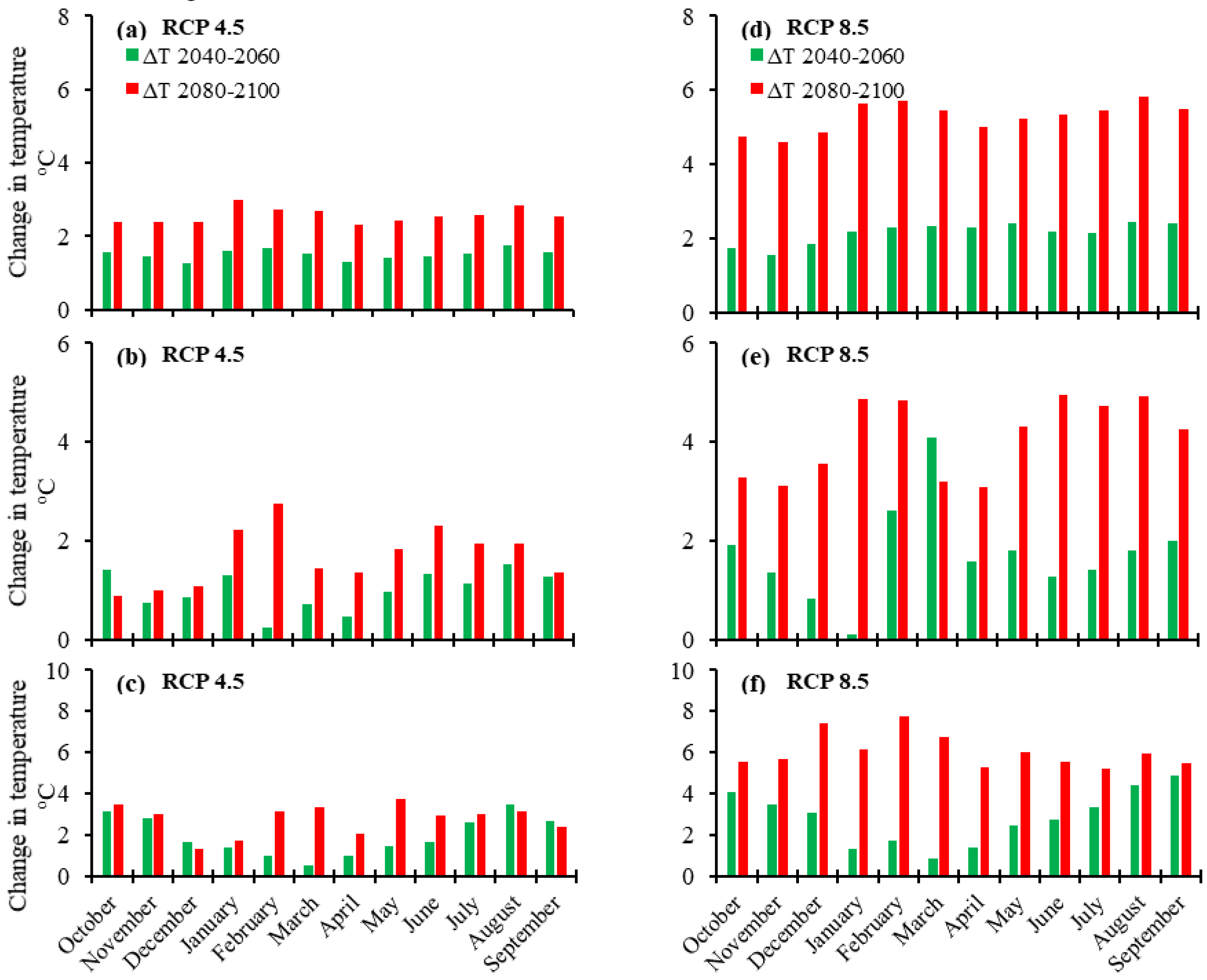
In the present study, eight GCMs were used to obtain temperature and precipitation in the future climate under RCP 4.5, a medium stabilization scenario, and RCP 8.5, a very high baseline emission scenario [75]. Figure 4 and Figure 5 show the average, lower, and higher temperature and precipitation changes, respectively, projected by the GCMs for the mid-21st century (2040–2060) and late 21st century (2080–2100). Temperature is projected to increase under both RCPs, whereas precipitation is projected to decrease in the future with respect to the baseline period (2000–2020). The mean monthly projected temperatures of all GCMs under the RCP 4.5 and 8.5 emission scenarios show increases in all months during both 2040–2060 and 2080–2100.
Under RCP 4.5, the minimum average monthly temperature rise was 1.3 °C in December and April during 2040–2060, and 2.3 °C in April during 2080–2100. The maximum value average monthly temperature rise was 1.7 °C in February and August during 2040–2060, and 3 °C in January during 2080–2100, under RCP4.5 (Figure 4). Under RCP 8.5, the minimum rise in average temperature was 1.6 °C and 4.6 °C in November and the maximum rise was 2.5 °C and 5.8 °C in August, during 2040–2060 and 2080–2100, respectively (Figure 4).
Figure 4 also shows the monthly temperature increases projected by the GCMs assuming lower uncertainty under both emission scenarios and over the same periods. Under RCP 4.5, the mean lower monthly temperature is projected to increase by 0.2–1.5 °C and 0.9–2.7 °C, and under RCP 8.5, by 0.1–4.1 °C and 3.1–4.9 °C, during 2040–2060 and 2080–2100, respectively. Further, the future mean higher monthly temperature increases under RCP 4.5 are likely to be 0.5–3.5 °C and 1.3–3.7 °C and those under RCP 8.5 are likely to be 0.8–4.9 °C and 5.2–7.7 °C during 2040–2060 and 2080–2100, respectively. Overall, temperature is expected to significantly increase in the winter (January and February) and summer (July–September) months under RCP 8.5 (Figure 4). Previous climate change studies in Himalayan basins also suggest greater warming during winter [76,77]. Also, increases in winter and summer temperatures have similar trends to a previous finding over the same region under both scenarios [15]. Sanjay et al. reported an increase in temperature over the Hindukush and Karakoram using regional climate models, namely by 5.4 °C during winter and of 4.9 °C during summer season by the end of 21st century under the RCP8.5 scenario [78].
The projected precipitation changes mainly show decreases, compared to the baseline period, under both RCP 4.5 and 8.5 (Figure 5). Mean monthly precipitation will likely decline by 1.1% to 12.3% under RCP 4.5 and by 1.2% to 13% under RCP 8.5, with the largest declines occurring from December to March. Increases of 0.1% to 29% in mean monthly precipitation were simulated, mostly between June and September, under both emission scenarios. Mean lower monthly precipitation decreased by 1.6% to 34% under both RCP 4.5 and 8.5, whereas significant increases in the mean higher monthly precipitation ranged from 0.4% to 231%. The projected precipitation amounts showed large month-to-month variation. A study has also indicated that the variation of precipitation in most climate models is increasing in response to the warming over a majority of the global land area [79]. The variation in precipitation also connects extreme wet and dry incidents, floods, and droughts that raise threats to the climate and community [79]. Overall, precipitation is likely to decrease during winter (December–February), but to increase during the summer months (Figure 5). Decreasing precipitation trends, particularly in wintertime (December–March), have been reported previously in the western Himalaya [12,15]. Buda et al. projected decreases in winter and spring precipitation in the Indus River Basin by 7.9% and 2.71% under RCP 4.5 and decrease by 9.0% and 10.1% under RCP 8.5 towards the mid- and end of this century, respectively [14]. Similarly, Amin et al. projected a reduction in winter precipitation and an increase in summer precipitation over southern Punjab during the near and mid of this century for 4.5, 6, and 8.5 scenarios [80].

4.4.2. Projected Snow Cover Area Distribution

It is very important to understand the impact of climate change on the snow cover area distribution, especially in snow-dominated high-altitude basins. The effect of climate change on the SCA in the Panjshir sub-basin during the mid- and late 21st century was simulated by the SM under RCP 4.5 and 8.5. The SCA simulated by the SM for 2009–2015 was used as the baseline value for projecting future SCA changes during 2049–2055 and 2089–2095. These particular years were selected to represent the years during the mid and late 21st century based on the baseline period.
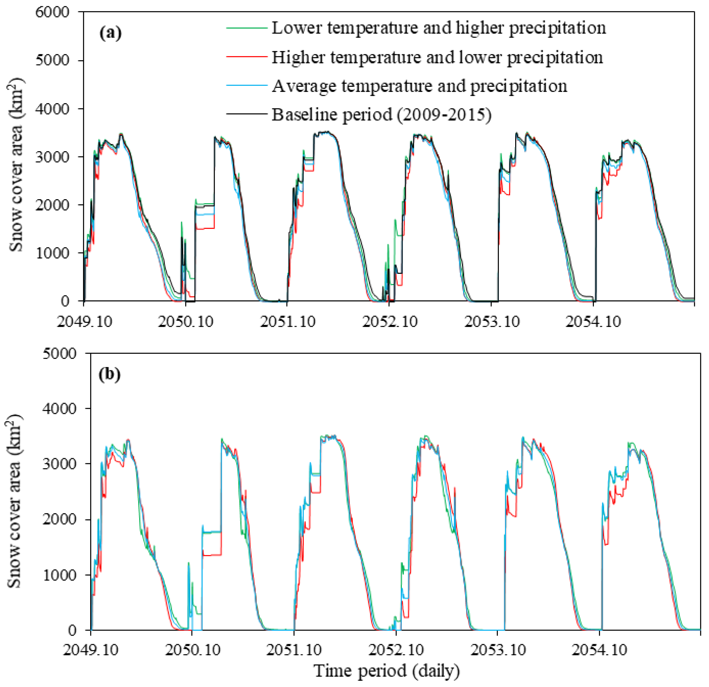
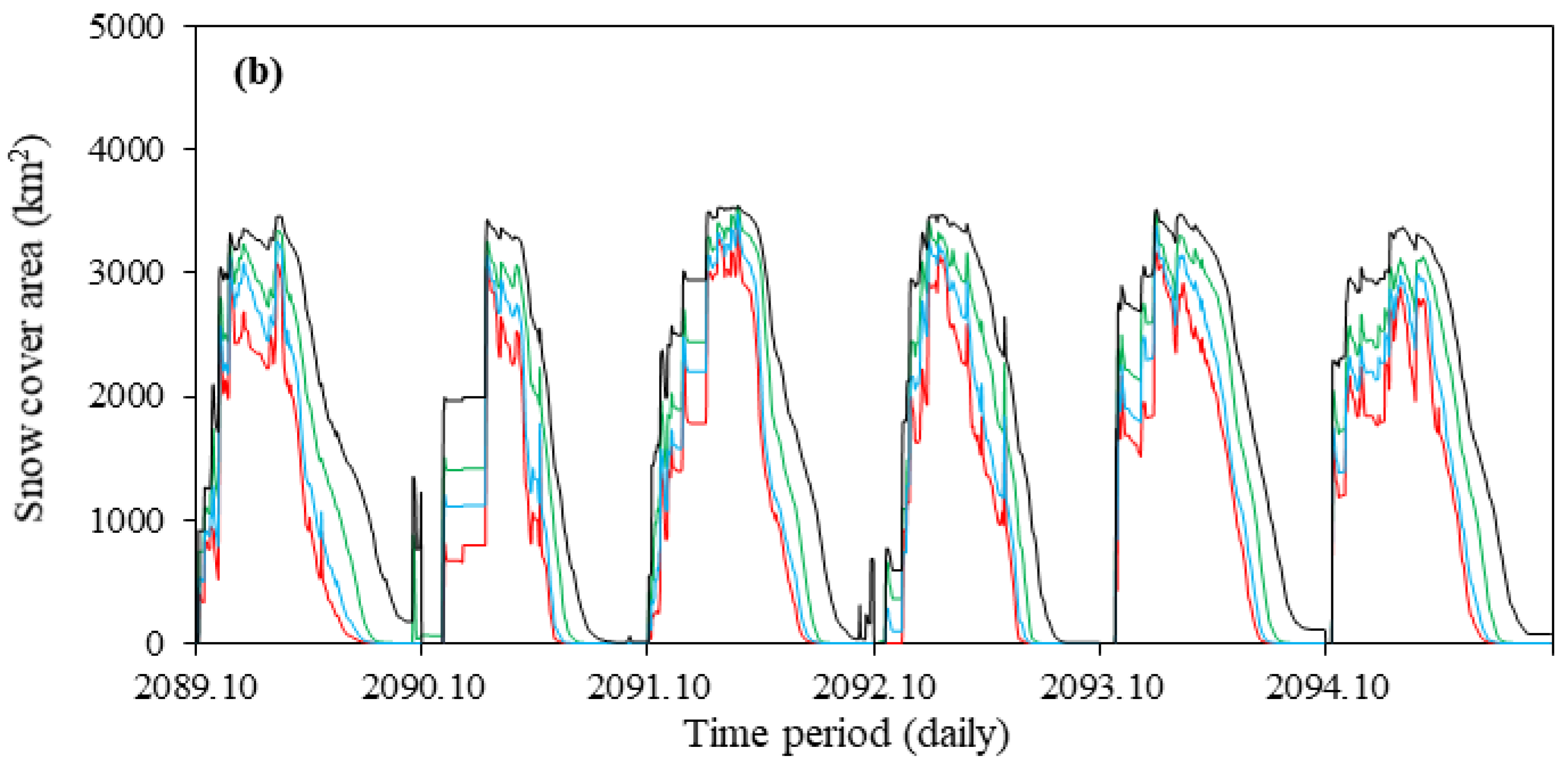
Average, lower, and higher temperature and precipitation climate change scenarios were used to simulate future daily SCAs. Using average temperature and precipitation scenarios during 2049–2055, SM simulations projected that the average annual SCA will decline by 7% (132 km2) under RCP 4.5, and by 12% (210 km2) under RCP 8.5 (Figure 6). Using lower temperature and higher precipitation scenarios, SM simulations projected a decrease in the annual average SCA of 0.15% (3 km2) under RCP 4.5 and of 10% (192 km2) under RCP 8.5 during 2049–2055. Similarly, based on higher temperature and lower precipitation scenarios, the annual average SCA was projected to decline by 8% (152 km2) and 15% (283 km2) under RCP 4.5 and 8.5, respectively (Figure 6).
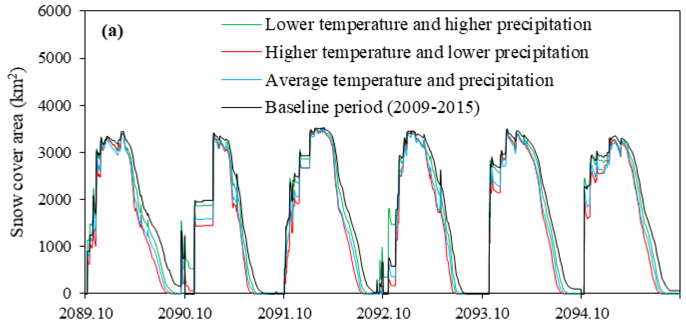
Based on average temperature and precipitation scenarios, the simulated SCA under RCP 4.5 and 8.5 decreased by 15% (279 km2) and 34% (152 km2), respectively, during 2089–2095 (Figure 7).
Based on lower temperature and higher precipitation scenarios, the simulated annual average SCA during 2089–2095 was reduced under RCP 4.5 and 8.5 by 6% (115 km2) and 21% (378 km2), respectively, and for higher temperature and lower precipitation scenarios, the simulated annual average SCA during the same period was reduced by 19% (346 km2) and 44% (806 km2), respectively. Moreover, the SCA was projected to decline during most seasons during the mid- and late 21st century under both RCPs (Table 5). Based on average temperature and precipitation scenarios, and higher temperature and lower precipitation scenarios, in all seasons, the minimum SCA reduction during 2049–2055 was seen under RCP 4.5, and the maximum SCA reduction during 2089–2095 was seen under RCP 8.5 (Table 5). Based on lower temperature and higher precipitation scenarios, however, the SCA increased by 108 km2 and 67 km2 in autumn during 2049–2055 under RCP 4.5 and 8.5, respectively, whereas during 2089–2095, the SCA in autumn decreased by 53 km2 under RCP 4.5 and by 348 km2 under RCP 8.5 (Table 5). In the same manner, the wintertime SCA during 2049–2055 increased by only 3 km2 under RCP 4.5, whereas it decreased by 128 km2 under RCP 8.5. Under both RCPs, the SCA declined by 60–614 km2 and 61–242 km2 in spring and summer, respectively, during both the mid- and late century (Table 5). Similar trends were projected in the snow cover area with the largest decrease in spring followed by winter in HKH in the mid of the 21st century [18].
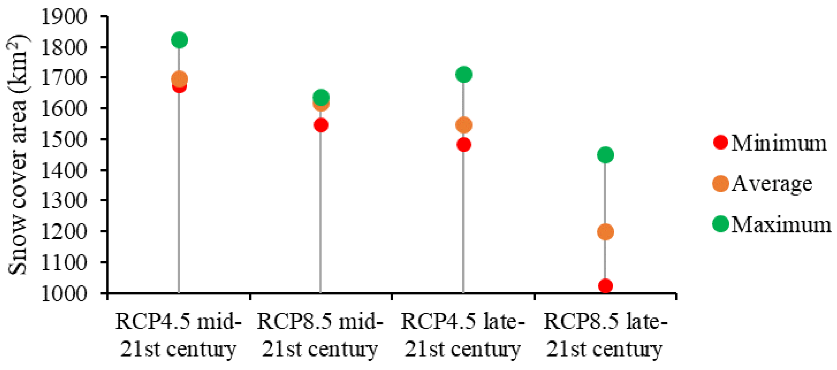
Figure 8 shows the range of uncertainty for the projected SCA in the eight GCMs. Under RCP 8.5, the lowest and highest uncertainty in the projected SCA was seen during the mid- and late 21st century, respectively. Under RCP 4.5, the range of uncertainty was also lower during the mid-century than during the late century. Under RCP 8.5, SCA ranged from about 1547 km2 to 1638 km2 in the mid-century and from 1023 km2 to 1451 km2 in the late century. Under RCP 4.5, SCA ranged from about 1677 km2 to 1826 km2 and from 1483 km2 to 1714 km2 in the mid- and late century, respectively.
In general, SCA was reduced across all scenarios. The projected increases in winter temperature and decreases in winter precipitation caused the wintertime snow cover in the study area to decline [18], and this decline will likely affect the timing and rate of snowmelt. The extent of glacier ice and the number of snow cover days are expected to decrease or even vanish during the 21st century [81]. In addition, basins with low percentages of glacier cover will be transformed from snow-dominated to rain-dominated, and this transformation is expected to shift the main runoff season from summer to winter [81].

4.4.3. Projected River Flows

In this section we address the impacts of climate change on river flows in the Panjshir sub-basin. Projected river flows during the mid- and late 21st century were simulated with the SRM under the RCP 4.5 and 8.5 scenarios. The discharge simulated by the SRM for 2009–2015 was used as the baseline for the projected daily flows during 2049–2055 and 2089–2095. Further, we used the average, lower, and higher temperature and precipitation scenarios from the eight GCMs and the resulting simulated SCAs to simulate daily flows under both climate scenarios.
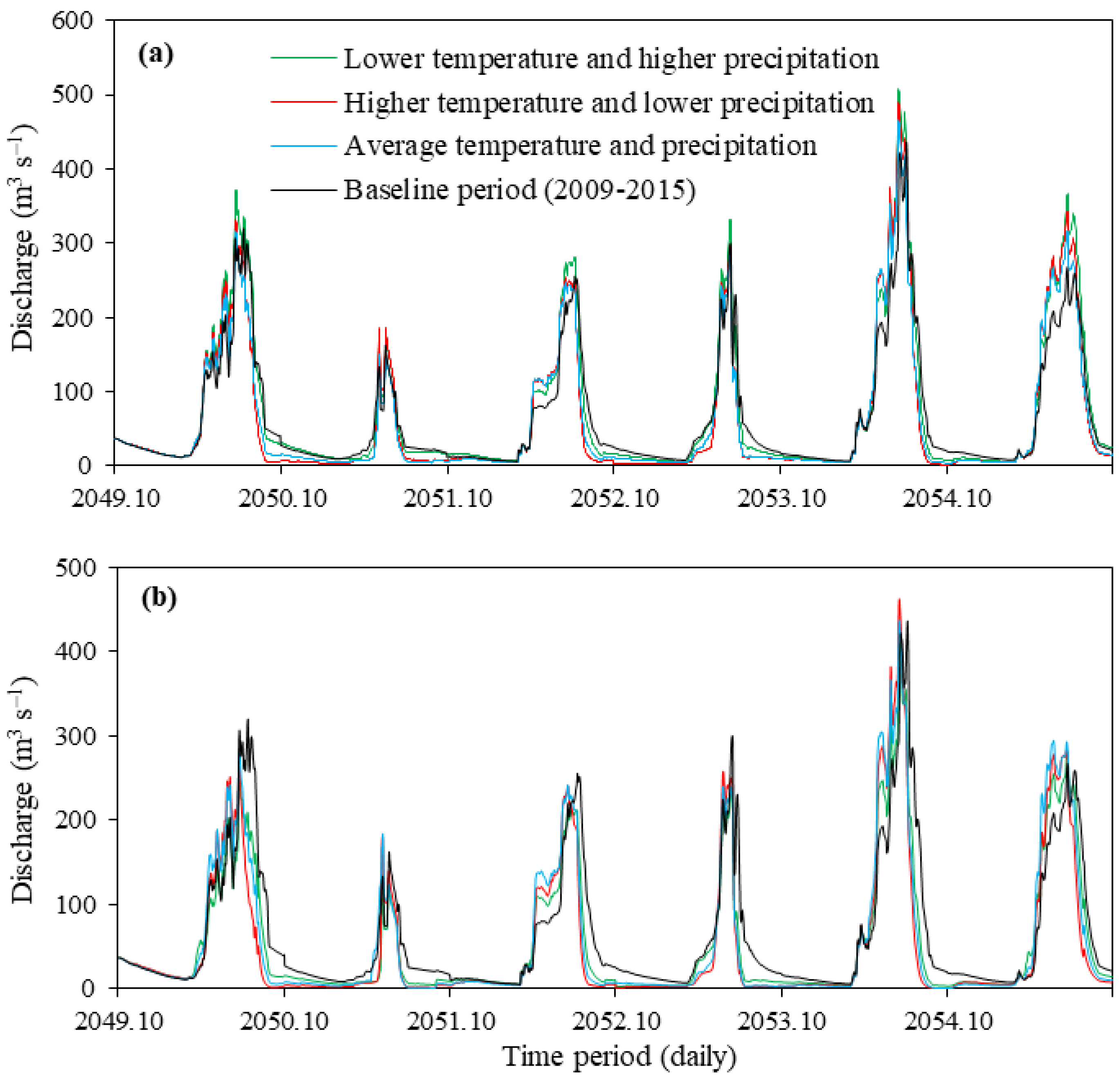
Figure 9 presents daily projected flows during 2049–2055 in the Panjshir sub-basin under RCP 4.5 and 8.5, obtained by using the average, lower, and higher temperature and precipitation scenarios and the resulting simulated SCAs. The SRM simulation results based on the average temperature and precipitation scenarios indicate that the annual average discharge during 2049–2055 will decrease by about 7% (5 m3 s–1) and 13% (9 m3 s–1) under RCP 4.5 and 8.5, respectively. Based on the lower temperature and higher precipitation scenarios, the annual average discharge during 2049–2055 is projected to increase under RCP 4.5 by 9% (6 m3 s–1), whereas under RCP 8.5, it is projected to decrease by 17% (11 m3 s–1). Moreover, based on the higher temperature and lower precipitation scenarios, the annual average discharge during 2049–2055 is projected to decrease by 6% (4 m3 s–1) and 21% (14 m3 s–1) under RCP 4.5 and 8.5, respectively (Figure 9).
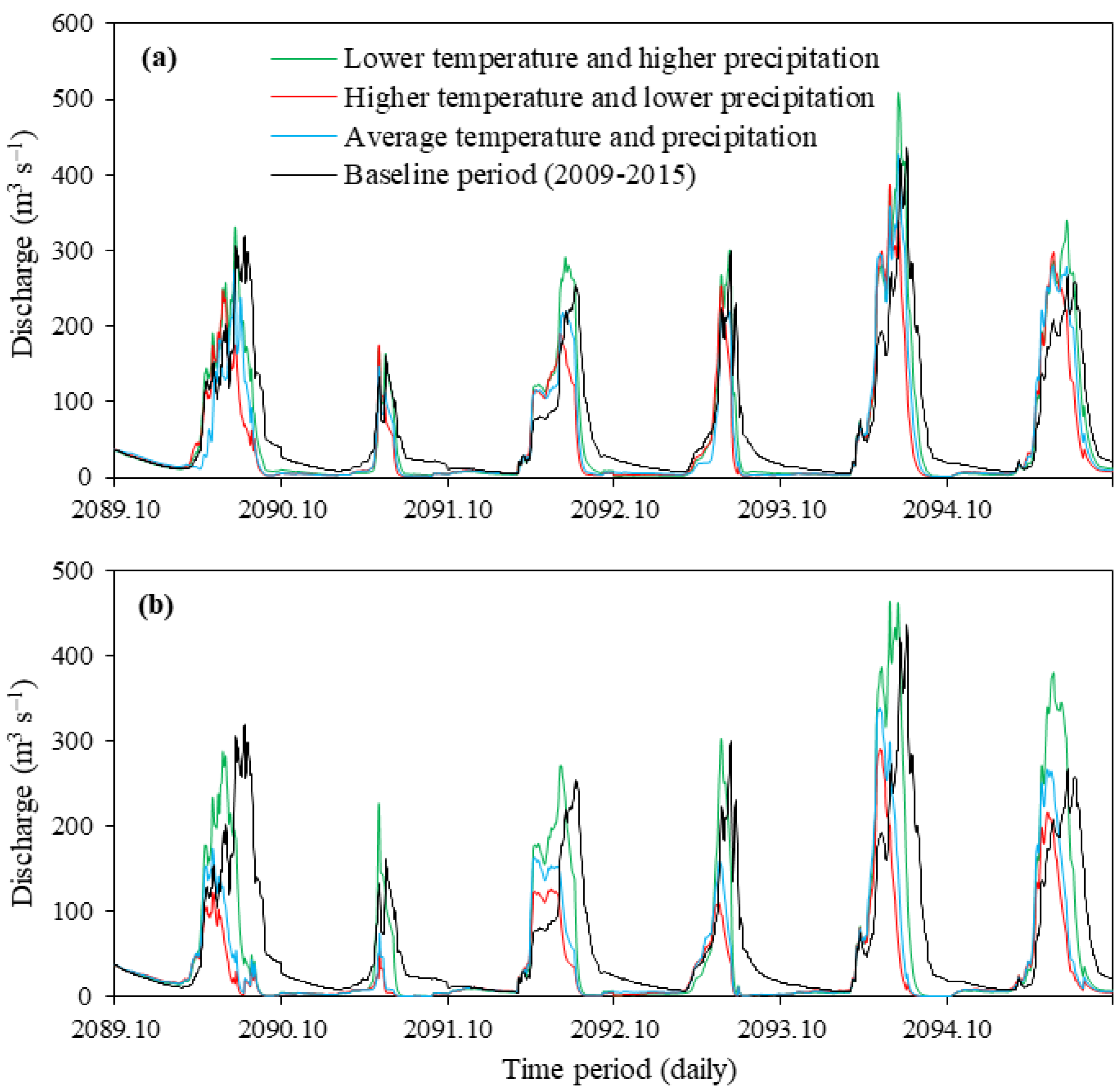
A decrease of 25% (16 m3 s–1) under RCP 4.5 and as much as 43% (27 m3 s–1) in the annual average discharge during 2089–2095 was projected under RCP 8.5, based on the average temperature and precipitation scenarios and the resulting SCAs (Figure 10). Based on the lower temperature and higher precipitation scenarios, the projected decreases were about 7% (4 m3 s–1) and 17% (11 m3 s–1) under RCP 4.5 and 8.5. The largest projected reductions in annual average discharge during the late 21st century of approximately 31% (20 m3 s–1) under RCP 4.5, and 55% (35 m3 s–1) under RCP 8.5, were obtained by using the higher temperature and lower precipitation scenarios.
Furthermore, significant changes in the projected seasonal river discharge during the mid- and late century were seen across all climate change scenarios (Table 6). Based on average temperature and precipitation scenarios, the springtime discharge was projected to increase by 20 m3 s–1 in the mid-century and by 5 m3 s–1 in the late century under RCP 4.5. Under RCP 8.5, the discharge was projected to increase by 25 m3 s–1 in the mid-century, but to decline by 20 m3 s–1 in the late century (Table 6). Based on the higher temperature and lower precipitation scenarios, the discharge was projected to decrease by 3–9 m3 s–1 except during the late century under RCP 8.5, when it was projected to increase by 1 m3 s–1. Based on the lower temperature and higher precipitation scenarios, the discharge was projected to decrease slightly in autumn and winter, whereas a large summertime decrease was projected. However, in spring, the discharge was projected to increase under both RCP 4.5 and 8.5 in the mid- and late century (Table 6).
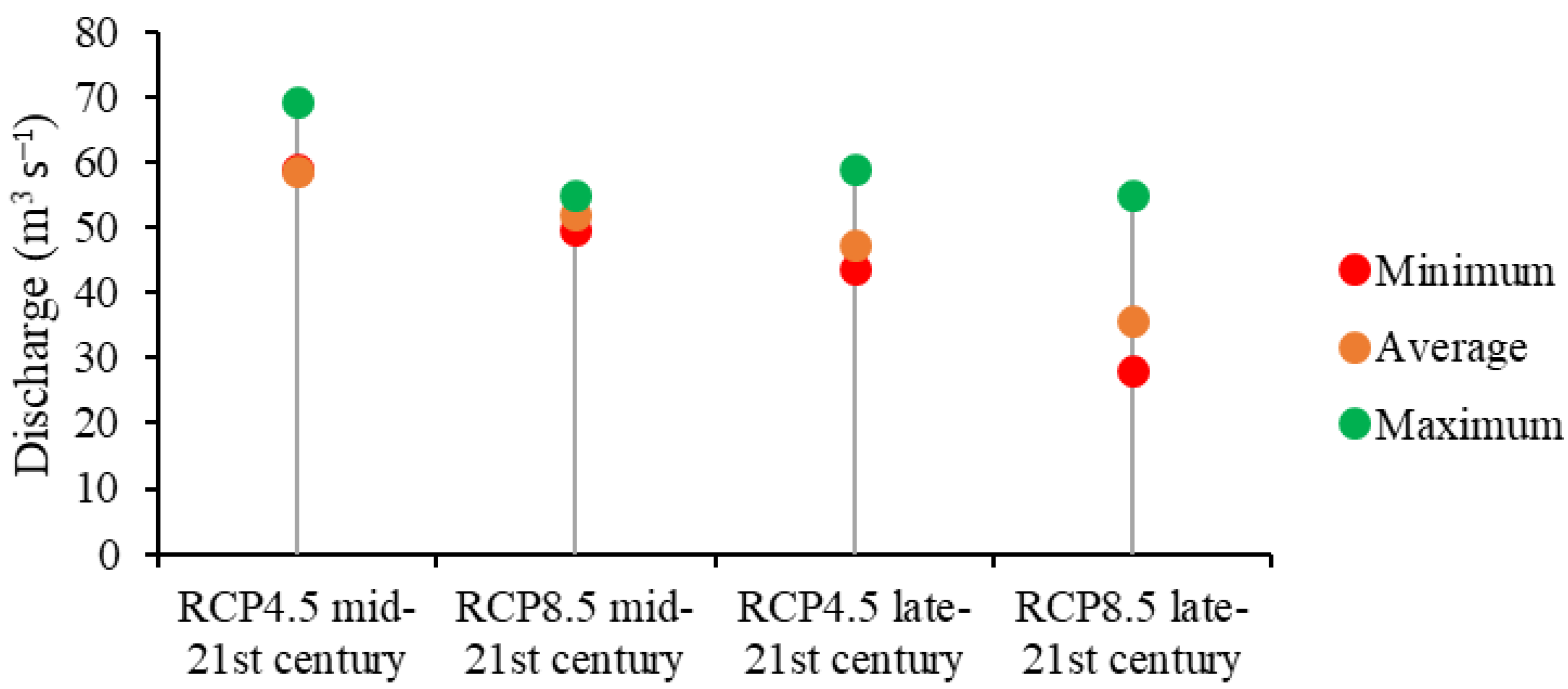
Figure 11 depicts the range of uncertainty in the projected river discharge for the eight GCMs. Similar to the projected SCA, the smallest uncertainty range in river discharge was seen in the mid-century under RCP 8.5, and the largest range was seen in the late century under RCP 8.5. Under RCP 4.5, the uncertainty range was also small in the mid-century and large in the late century. The smallest and largest uncertainty ranges under RCP 4.5 were 59 and 69 m3 s–1, respectively, in the mid-century, and 44 and 59 m3 s–1, respectively, in the late century. Under RCP 8.5, the smallest and largest uncertainty ranges were 50 and 55 m3 s–1, respectively, during the mid-century, and 28 and 55 m3 s–1, respectively, during the late century.
In general, the simulated river flows decreased relative to the baseline period during the mid- and late 21st century under both RCP scenarios, based on average, lower, and higher temperature and precipitation scenarios, except under RCP 4.5 and the lower temperature and higher precipitation scenarios, when river flow showed a slight increase. These results suggest that less snow will accumulate in winter and river flows will peak earlier in spring. In particular, the remarkable shifts seen under RCP 8.5 will likely cause extreme flooding events in the study area to shift from summer (July–August) to spring (April–June). The increasing temperature may contribute to the rapid melting of the ice, which may raise flood frequency and intensity [28], and flash and river floods in the Hindukush area pose the most hazards [42]. The simulation results also indicate that river flows will decline in late summer, when demand is highest, thus increasing the risk of drought. Soncini et al. also suggested that river discharge remains high in spring and decrease in July and August towards the end of the century [82]. Other studies have also reported that the flow regime in snow-dominated basins is more sensitive to a wintertime temperature rise because of a similar shift [83].

4.4.4. Projected Flow Regime

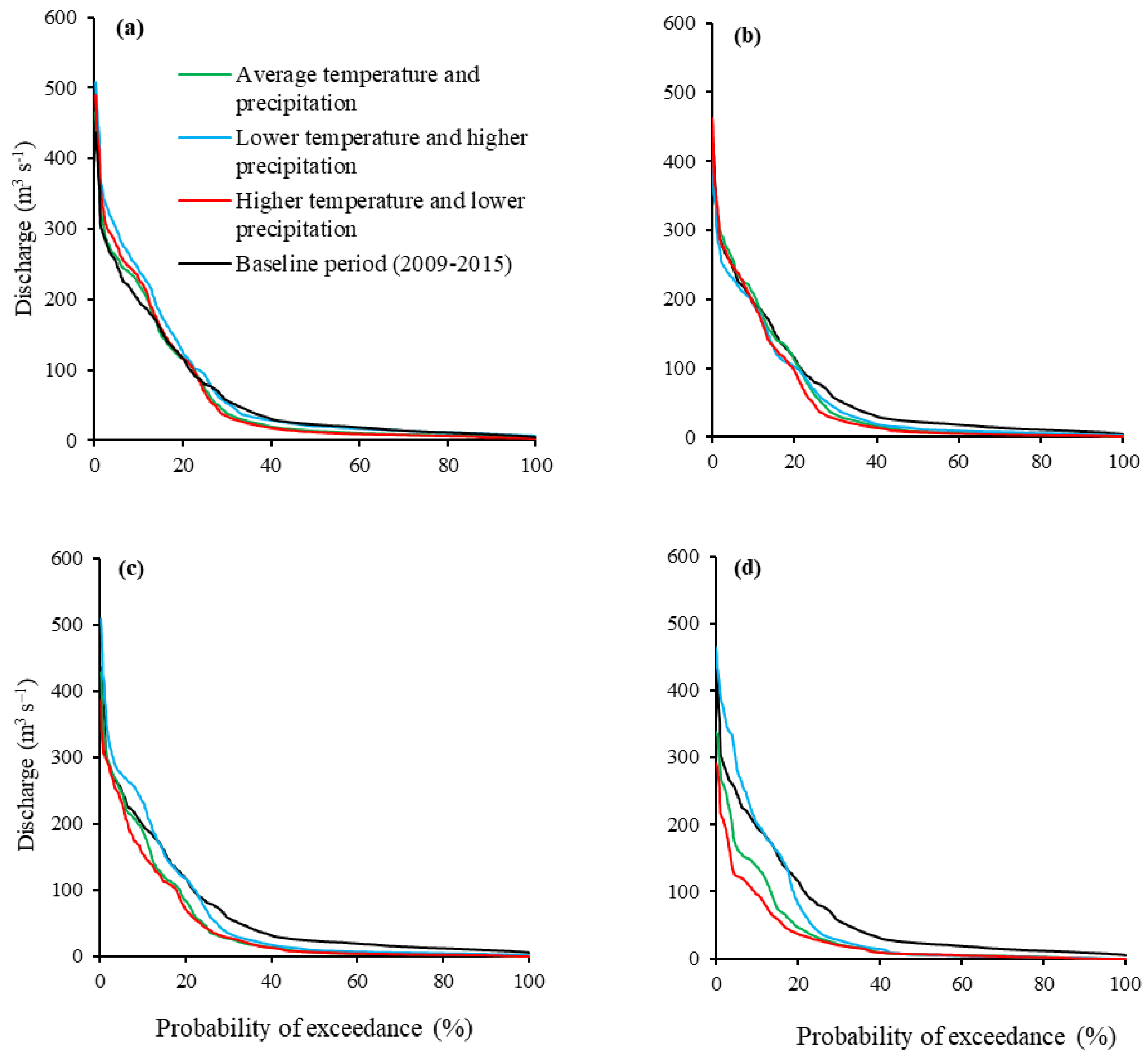
Flow duration curves (FDCs) were constructed for the mid- and late 21st century by using the simulated daily output under the climate change scenarios and compared them with the FDC for the baseline period to evaluate changes in exceedance flows (Figure 12). We define flow rates between Q0 and Q20 as high flow rates, and consider ones from Q0 to Q15 to indicate extreme flood events, where Q is discharge and the numerical subscript indicates the exceedance probability—the percentage chance that the discharge will be equaled or exceeded in any given year. Simulation results showed that during 2049–2055, the probability of high flows (Q0–Q20) increased, relative to the baseline period, under all three climate change scenarios (average temperature and precipitation; lower temperature and higher precipitation; and higher temperature and lower precipitation) under RCP 4.5, whereas under RCP 8.5, the probability of flows below Q10 was about the same and the probability of flows below Q20 was slightly decreased.
However, under both RCPs during 2089–2095, the probability of flows below Q15 increased relative to the baseline period only under the lower temperature and higher precipitation scenario; under the other scenarios, the probability was significantly decreased. Under all scenarios, the probability of flows above Q80 tended to be similar.
In general, low flows will occur more frequently in the future, and high flows will occur less frequently. Thus, climate change will likely reduce the overall flow regime in the Panjshir sub-basin. The significant drop in upstream discharges will have consequences for people in downstream areas, who will likely experience severe water shortages in the future.

5. Conclusions

The main objective of this study was to simulate the effects of climate change on the snow cover area distribution and river flows in the Panjshir sub-basin that can be expected during the 21st century. To achieve this objective, we used the SM to simulate daily SCA. Then we used the SRM to simulate river flows in the Panjshir sub-basin.
Calibrated and validated models were used with climate change scenarios to project the future changes in the SCA distribution and river flows in the Panjshir sub-basin. Climate projection datasets under the RCP 4.5 and 8.5 emission scenarios were utilized to assess the expected changes in climate variables. Mean annual temperature was projected to increase by 1.45 °C and 2.51 °C under RCP 4.5 and by 2.05 °C and 5.18 °C under RCP 8.5 during the mid and late 21st century, respectively. Precipitation was projected to decrease by 4.7% and 5.4% under RCP 4.5 and by 1.7% and 4.4% under RCP 8.5 during the same respective periods.
The simulated mean annual SCA based on lower, average, and higher temperature and precipitation scenarios was decreased under RCP 4.5 and 8.5 during 2049–2055 and 2089–2095. The projected runoff was also projected to decrease under RCP 4.5 and 8.5 during 2049–2055 and 2089–2095, except for the lower temperature and higher precipitation scenario, which projected a runoff increase of only 9% under RCP 4.5 during 2049–2055. The future SCA was projected to decrease in all seasons in the mid- and late century using all climate change scenarios, except for a projected increase in autumn of 67 km2 during the late century under RCP 4.5. River discharge was projected to decrease, except in spring, when it was projected to increase in the mid-century under both RCPs. Under RCP 8.5, the range of uncertainty for projected SCA and river discharge was smallest in the mid-century and largest in the late century. In addition, the number of days with low flows was projected to increase in the future, and the probability of high flows was projected to decrease by about 10%. Changes in future SCA and stream flows are expected to alter the Panjshir sub-basin hydrology and may significantly influence the demand for water for agricultural irrigation, the domestic water supply, hydropower generation, and natural ecosystems, particularly in downstream areas.
The objective of this study was to quantify the impacts of climate change on future SCA and stream flow in a data-scarce snow-dominated basin in the Hindukush–Himalaya region. SM and SRM were applied with a limited number of years due to data-scarcity over which the simulations are calibrated and validated, which may remain some uncertainties in this study. The modeling method used has some limitations as well, which decreases its accuracy over time with an increasing temporal resolution, and it cannot accurately model the spatial variability as melting rates may differ due to topographic effects [66].
Future work is needed to update the research by accessible observations particularly for higher altitudes of the study area which will further improve the results of hydrological modeling. A case for further studies to deal with water management and decision-making on the sub-basin scale in Afghanistan can be made based on the study proposed here to better respond with some adaptation plans to changing future water availability.

Supplementary Materials

The following are available online at https://www.mdpi.com/2306-5338/7/4/74/s1, Figure S1. Zone-wise comparison between MODIS observed and simulated SCAs during the (a) calibration and (b) validation periods., Figure S2. Basin-wide daily SCA simulated by the SM compared with the MODIS observed SCA during the calibration and validation periods., Figure S3. Comparison of the distributions of SCA simulated by the SM and MODIS observed SCA during the (a) one calibration and (b) five validation years., Figure S4. Times series of daily observed discharge and discharge simulated by using simulated SCA values during the calibration and validation periods., Figure S5. Scatter plot between observed daily discharge and daily discharge simulated with the SRM; the solid and dashed lines corresponds the regression and 1:1 line, respectively., Table S1. SM parameters used for current and future simulations., Table S2. SRM parameters and variables used for current and future simulations., Table S3. Optimized DDF and PG values in each elevation zone in the study area., Table S4. Zone-wise parameter values used in applying SRM for runoff simulation., Table S5. Performance of the SRM in simulating river discharge during the calibration and validation periods.

Author Contributions

Conceptualization, A.H.A. and Y.A.; methodology, A.H.A. and Y.A.; software, A.H.A. and Y.A.; validation, A.H.A. and Y.A.; formal analysis, A.H.A.; investigation, A.H.A.; resources, A.H.A. and Y.A.; data curation, A.H.A.; writing—original draft preparation, A.H.A.; writing—review and editing, A.H.A. and Y.A.; visualization, A.H.A.; supervision, Y.A.; project administration, Y.A.; funding acquisition, Y.A. All authors have read and agreed to the published version of the manuscript.

Funding

This research was funded by a JICA special program, JSPS KAKENHI Grant Number 20K04712, and JSPS Open Partnership Joint Research Projects.

Acknowledgments

The authors thank the National Water Affairs Regulation Authority for providing hydrological and meteorological data. We are grateful to the anonymous reviewers whose comments and suggestions significantly improved the manuscript.

Conflicts of Interest

The authors declare no conflict of interest.

References

  1. Haddeland, I.; Heinke, J.; Biemans, H.; Eisner, S.; Florke, M.F.; Hanasaki, N.; Konzmann, M.; Ludwig, F. Global water resources affected by human interventionss and climate change. Proc. Natl. Acad. Sci. USA 2014, 111, 3251–3256. [Google Scholar] [CrossRef] [Green Version]
  2. Nepal, S. Impacts of climate change on the hydrological regime of the Koshi river basin in the Himalayan region. J. Hydro-Environ. Res. 2016, 10, 76–89. [Google Scholar] [CrossRef] [Green Version]
  3. You, Q.; Ren, G.Y.; Zhang, Y.Q.; Ren, Y.; Sun, X.B.; Zhan, Y.J.; Shrestha, A.B.; Krishnan, R. An overview of studies of observed climate change in the Hindu Kush Himalayan (HKH) region. Adv. Clim. Chang. Res. 2017, 8, 141–147. [Google Scholar] [CrossRef]
  4. Kumar, P.; Kotlarski, S.; Moseley, C.; Sieck, K.; Frey, H.; Stoffel, M.; Jacob, D. Response of Karakoram-Himalayan glaciers to climate variability and climatic change: A regional climate model assessment. Geophys. Res. Lett. 2015, 42, 1818–1825. [Google Scholar] [CrossRef]
  5. Pelto, M. Recent Climate Change Impacts on Mountain Glaciers. Available online: https://search.ebscohost.com/login.aspx?direct=true&scope=site&db=nlebk&db=nlabk&AN=1412837 (accessed on 1 September 2020).
  6. Shrestha, S.; Nepal, S. Water Balance Assessment under Different Glacier Coverage Scenarios in the Hunza Basin. Water 2019, 11, 1124. [Google Scholar] [CrossRef] [Green Version]
  7. Williams, M.W. The Status of Glaciers in the Hindu Kush–Himalayan Region. Mt. Res. Dev. 2013, 33, 114–115. [Google Scholar] [CrossRef]
  8. Bajracharya, S.R.; Maharjan, S.B.; Shrestha, F.; Guo, W.Q.; Liu, S.; Immerzeel, W.W.; Shrestha, B. The glaciers of the Hindu Kush Himalayas: Current status and observed changes from the 1980s to 2010. Int. J. Water Resour. Dev. 2015, 31, 161–173. [Google Scholar] [CrossRef] [Green Version]
  9. Mukherji, A.; Molden, D.; Nepal, S.; Rasul, G.; Wagnon, P. Himalayan waters at the crossroads: Issues and challenges. Int. J. Water Resour. Dev. 2015, 31, 151–160. [Google Scholar] [CrossRef] [Green Version]
  10. Nepal, S.; Shrestha, A.B. Impact of climate change on the hydrological regime of the Indus, Ganges and Brahmaputra river basins: A review of the literature. Int. J. Water Resour. Dev. 2015, 31, 201–218. [Google Scholar] [CrossRef] [Green Version]
  11. Prasad, A.K.; Yang, K.H.S.; El-Askary, H.; Kafatos, M. Melting of major Glaciers in the western Himalayas: Evidence of climatic changes from long term MSU derived tropospheric temperature trend (1979–2008). Ann. Geophys. 2009, 27, 4505–4519. [Google Scholar] [CrossRef] [Green Version]
  12. Lutz, A.F.; Ter Maat, H.W.; Biemans, H.; Shrestha, A.B.; Wester, P.; Immerzeel, W.W. Selecting representative climate models for climate change impact studies: An advanced envelope-based selection approach. Int. J. Clim. 2016, 36, 3988–4005. [Google Scholar] [CrossRef] [Green Version]
  13. Lutz, A.F.; Ter Maat, H.W.; Wijngaard, R.R.; Biemans, H.; Syed, A.; Shrestha, A.B.; Wester, P.; Immerzeel, W.W. South Asian river basins in a 1.5 °C warmer world. Reg. Environ. Chang. 2018, 19, 833–847. [Google Scholar] [CrossRef] [Green Version]
  14. Su, B.; Huang, J.; Gemmer, M.; Jian, D.; Tao, H.; Jiang, T.; Zhao, C. Statistical downscaling of CMIP5 multi-model ensemble for projected changes of climate in the Indus River Basin. Atmos. Res. 2016, 178, 138–149. [Google Scholar] [CrossRef]
  15. Bokhari, S.A.A.; Ahmad, B.; Ali, J.; Ahmad, S.; Mushtaq, H.; Rasul, G. Future Climate Change Projections of the Kabul River Basin using a Multi-model Ensemble of High-Resolution Statistically Downscaled Data. Earth Syst. Environ. 2018, 2, 477–497. [Google Scholar] [CrossRef]
  16. Muhammad, A.; Evenson, G.R.; Unduche, F.; Stadnyk, T.A. Climate Change Impacts on Reservoir Inflow in the Prairie Pothole Region: A Watershed Model Analysis. Water 2020, 12, 271. [Google Scholar] [CrossRef] [Green Version]
  17. Jiang, T.; Fischer, T.; Lu, X. Larger Asian rivers: Climate, hydrology and ecosystems. Quat. Int. 2011, 244, 127–129. [Google Scholar] [CrossRef]
  18. Khadka, D.; Babel, M.S.; Shrestha, S.; Tripathi, N.K. Climate change impact on glacier and snow melt and runoff in Tamakoshi basin in the Hindu Kush Himalayan (HKH) region. J. Hydrol. 2014, 511, 49–60. [Google Scholar] [CrossRef]
  19. Armstrong, R.L.; Rittger, K.; Brodzik, M.J.; Racoviteanu, A.; Barrett, A.P.; Khalsa, S.J.S.; Raup, B.; Hill, A.F.; Khan, A.L.; Wilson, A.M.; et al. Runoff from glacier ice and seasonal snow in High Asia: Separating melt water sources in river flow. Reg. Environ. Chang. 2018, 19, 1249–1261. [Google Scholar] [CrossRef] [Green Version]
  20. Immerzeel, W.W.; Droogers, P.; de Jong, S.M.; Bierkens, M. Large-scale monitoring of snow cover and runoff simulation in Himalayan river basins using remote sensing. Remote. Sens. Environ. 2009, 113, 40–49. [Google Scholar] [CrossRef]
  21. Kour, R.; Patel, N.; Krishna, A.P. Assessment of temporal dynamics of snow cover and its validation with hydro-meteorological data in parts of Chenab Basin, western Himalayas. Sci. China Earth Sci. 2016, 59, 1081–1094. [Google Scholar] [CrossRef]
  22. Winiger, M.; Gumpert, M.; Yamout, H. Karakorum-Hindukush-western Himalaya: Assessing high-altitude water resources. Hydrol. Process. 2005, 19, 2329–2338. [Google Scholar] [CrossRef]
  23. Hasson, S.U.; Böhner, J.; Lucarini, V. Prevailing climatic trends and runoff response from Hindukush–Karakoram–Himalaya, upper Indus Basin. Earth Syst. Dyn. 2017, 8, 337–355. [Google Scholar] [CrossRef] [Green Version]
  24. Immerzeel, W.W.; van Beek, L.P.H.; Bierkens, M.F.P. Climate Change Will Affect the Asian Water Towers. Science 2010, 328, 1382–1385. [Google Scholar] [CrossRef]
  25. Immerzeel, W.W.; van Beek, L.P.H.; Konz, M.; Shrestha, A.B.; Bierkens, M.F.P. Hydrological response to climate change in a glacierized catchment in the Himalayas. Clim. Chang. 2012, 110, 721–736. [Google Scholar] [CrossRef] [PubMed] [Green Version]
  26. Wang, J.; Li, S. Effect of climatic change on snowmelt runoffs in mountainous regions of inland rivers in Northwestern China. Sci. China Ser. D 2006, 49, 881–888. [Google Scholar] [CrossRef]
  27. Wijngaard, R.R. Climate Change in Mountainous River Basins: Understanding Climate Change Impacts and Challenges Across Different Spatial Scales. Ph.D. Thesis, Utrecht University, Uthrecht, The Netherlands, 2019. [Google Scholar]
  28. Hayat, H.; Akbar, T.A.; Tahir, A.A.; Hassan, Q.K.; Dewan, A.; Irshad, M. Simulating Current and Future River-Flows in the Karakoram and Himalayan Regions of Pakistan Using Snowmelt-Runoff Model and RCP Scenarios. Water 2019, 11, 761. [Google Scholar] [CrossRef] [Green Version]
  29. Brubaker, K.; Rango, A.; Kustas, W. Incorporating Radiation Inputs into the Snowmelt Runoff Model. Hydrol. Process. 1996, 10, 1329–1343. [Google Scholar] [CrossRef]
  30. Rajkumari, S.; Chiphang, N.; Kiba, L.G.; Bandyopadhyay, A.; Bhadra, A. Development and application of a spatially distributed snowmelt runoff model for limited data condition. Arab. J. Geosci. 2019, 12, 488. [Google Scholar] [CrossRef]
  31. Martinec, J.; Rango, A.; Roberts, R. Snowmelt Runoff Model (SRM) User’s Manual; New Mexico State University: Las Cruces, NM, USA, 2008. [Google Scholar]
  32. Zhang, G.; Xie, H.; Yao, T.; Li, H.; Duan, S. Quantitative water resources assessment of Qinghai Lake basin using Snowmelt Runoff Model (SRM). J. Hydrol. 2014, 519, 976–987. [Google Scholar] [CrossRef]
  33. Xie, S.; Du, J.; Zhou, X.; Zhang, X.; Feng, X.; Zheng, W.; Li, Z.; Xu, C.Y. A progressive segmented optimization algorithm for calibrating time-variant parameters of the snowmelt runoff model (SRM). J. Hydrol. 2018, 566, 470–483. [Google Scholar] [CrossRef]
  34. Butt, M.J.; Bilal, M. Application of snowmelt runoff model for water resource management. Hydrol. Process. 2011, 25, 3735–3747. [Google Scholar] [CrossRef]
  35. Panday, P.; Williams, C.A.; Frey, K.E.; Brown, M. Application and evaluation of a snowmelt runoff model in the Tamor River basin, Eastern Himalaya using a Markov Chain Monte Carlo (MCMC) data assimilation approach. Hydrol. Process. 2013, 28, 5337–5353. [Google Scholar] [CrossRef] [Green Version]
  36. Yu, M.; Chen, X.; Li, L.; Bao, A.; de La Paix, M.J. Incorporating accumulated temperature and algorithm of snow cover calculation into the snowmelt runoff model. Hydrol. Process. 2012, 27, 3589–3595. [Google Scholar] [CrossRef]
  37. Munir, M.B. Climate change impact on flow discharge of neelum river catchment using Snowmelt Runoff Model. In Proceedings of the IEEE International Conference on Space Science and Communication (IconSpace), Melaka, Malaysia, 1–3 July 2013; pp. 350–355. [Google Scholar]
  38. Tahir, A.A.; Hakeem, S.A.; Hu, T.; Hayat, H.; Yasir, M. Simulation of snowmelt-runoff under climate change scenarios in a data-scarce mountain environment. Int. J. Digit. Earth 2017, 12, 910–930. [Google Scholar] [CrossRef]
  39. Tahir, A.A.; Chevallier, P.; Arnaud, Y.; Neppel, L.; Ahmad, B. Modeling snowmelt-runoff under climate scenarios in the Hunza River basin, Karakoram Range, Northern Pakistan. J. Hydrol. 2011, 409, 104–117. [Google Scholar] [CrossRef]
  40. Adnan, M.; Nabi, G.; Poomee, M.S.; Ashraf, A. Snowmelt runoff prediction under changing climate in the Himalayan cryosphere: A case of Gilgit River Basin. Geosci. Front. 2017, 8, 941–949. [Google Scholar] [CrossRef] [Green Version]
  41. Adnan, M.; Nabi, G.; Kang, S.; Zhang, G.; Adnan, R.M.; Anjum, M.N.; Iqbal, M.; Ali, A.F. Snowmelt Runoff Modelling under Projected Climate Change Patterns in the Gilgit River Basin of Northern Pakistan. Pol. J. Environ. Stud. 2017, 26, 525–542. [Google Scholar] [CrossRef]
  42. Hayat, H.; Tahir, A.A.; Wajid, S.; Abbassi, A.M.; Zubair, F.; Hashmi, Z.U.R.; Khan, A.; Khan, A.J.; Irshad, M. Simulation of the meltwater under different climate change scenarios in a poorly gauged snow and glacier-fed chitral river catchment (Hindukush region). Geocarto Int. 2019, 1–17. [Google Scholar] [CrossRef]
  43. Azmat, M.; Qamar, M.U.; Huggel, C.; Hussain, E. Future climate and cryosphere impacts on the hydrology of a scarcely gauged catchment on the Jhelum river basin, Northern Pakistan. Sci. Total. Environ. 2018, 639, 961–976. [Google Scholar] [CrossRef]
  44. Khadka, A.; Devkota, L.; Kayastha, R. Impact of Climate Change on the Snow Hydrology of Koshi River Basin. J. Hydrol. Meteorol. 2016, 9, 28–44. [Google Scholar] [CrossRef] [Green Version]
  45. Ma, Y.; Huang, Y.; Chen, X.; Li, Y.P.; Bao, A. Modelling Snowmelt Runoff under Climate Change Scenarios in an Ungauged Mountainous Watershed, Northwest China. Math. Probl. Eng. 2013, 2013, 1–9. [Google Scholar] [CrossRef] [Green Version]
  46. Azizi, A.H.; Asaoka, Y. Incorporating snow model and snowmelt runoff model for streamflow simulation in a snow-dominated mountainous basin in the western Hindukush-Himalaya region. Hydrol. Res. Lett. 2020, 14, 34–40. [Google Scholar] [CrossRef] [Green Version]
  47. Azizi, A.H.; Asaoka, Y. Estimating spatial and temporal snow distribution using numerical model and satellite remote sensing in the western hindukush-himalaya region. Jpn. Soc. Civ. Eng. Ser. G 2019, 75, I_125–I_134. [Google Scholar] [CrossRef]
  48. Kazama, S.; Izumi, H.; Sarukkalige, P.R.; Nasu, T.; Sawamoto, M. Estimating snow distribution over a large area and its application for water resources. Hydrol. Process. 2008, 22, 2315–2324. [Google Scholar] [CrossRef]
  49. Asaoka, Y.; Kominami, Y. Spatial snowfall distribution in mountainous areas estimated with a snow model and satellite remote sensing. Hydrol. Res. Lett. 2012, 6, 1–6. [Google Scholar] [CrossRef] [Green Version]
  50. Asaoka, Y.; Kominami, Y. Incorporation of satellite-derived snow-cover area in spatial snowmelt modeling for a large area: Determination of a gridded degree-day factor. Ann. Glaciol. 2013, 54, 205–213. [Google Scholar] [CrossRef]
  51. Bajracharya, S.R.; Shrestha, B.R. The Status of Glaciers in the Hindu Kush-Himalayan Region; International Centre for Integrated Mountain Development (ICIMOD): Kathmandu, Nepal, 2011; pp. 24–29. [Google Scholar]
  52. Favre, R.; Kamal, G.M. Watershed Atlas of Afghanistan, 1st ed.; Working Document for Planners; Ministry of Irrigation Water Resources and Environment: Kabul, Afghanistan; Food and Agriculture Organization of the United Nations (FAO): Rome, Italy, 2004.
  53. Shroder, J.F. Watersheds of Want. In Natural Resources in Afghanistan; Chapter 5; Shroder, J.F., Ed.; Elsevier: Amsterdam, The Netherlands, 2014; pp. 138–180. [Google Scholar] [CrossRef]
  54. Akhtar, F.; Awan, U.K.; Tischbein, B.; Liaqat, U.W. Assessment of Irrigation Performance in Large River Basins under Data Scarce Environment—A Case of Kabul River Basin, Afghanistan. Remote. Sens. 2018, 10, 972. [Google Scholar] [CrossRef] [Green Version]
  55. Tachikawa, T.; Kaku, M.; Iwasaki, A.; Gesch, D.B.; Oimoen, M.J.; Zhang, Z.; Danielson, J.J.; Krieger, T.; Curtis, B.; Haase, J.; et al. ASTER Global Digital Elevation Model Version 2—Summary of Validation Results; NASA: Washington, DC, USA, 2011; p. 27.
  56. Akhtar, F.; Awan, U.K.; Tischbein, B.; Liaqat, U.W. A phenology based geo-informatics approach to map land use and land cover (2003–2013) by spatial segregation of large heterogenic river basins. Appl. Geogr. 2017, 88, 48–61. [Google Scholar] [CrossRef]
  57. Akhtar, F. Water Availability and Demand Analysis in the Kabul River Basin, Afghanistan. Ph.D. Thesis, University of Bonn, Bonn, Germany, 2017. [Google Scholar]
  58. Gurung, D.R.; Giriraj, A.; Aung, K.S.; Shrestha, B.R.; Kulkarni, A.V. Snow-Cover Mapping and Monitoring in the Hindu Kush-Himalayas; International Centre for Integrated Mountain Development (ICIMOD): Kathmandu, Nepal, 2011. [Google Scholar]
  59. Hall, D.K.; Riggs, G.A.; Salomonson, V.V.; Digirolamo, N.E.; Bayr, K.J. MODIS snow-cover products. Remote Sens. Environ. 2002, 83, 181–194. [Google Scholar] [CrossRef] [Green Version]
  60. Tekeli, A.E.; Akyürek, Z.; Şorman, A.A.; Şensoy, A. Using MODIS snow cover maps in modeling snowmelt runoff process in the eastern part of Turkey. Remote. Sens. Environ. 2005, 97, 216–230. [Google Scholar] [CrossRef]
  61. Karimi, H.; Zeinivand, H.; Tahmasebipour, N.; Haghizadeh, A.; Miryaghoubzadeh, M. Comparison of SRM and WetSpa models efficiency for snowmelt runoff simulation. Environ. Earth Sci. 2016, 75, 664. [Google Scholar] [CrossRef]
  62. Azmat, M.; Wahab, A.; Huggel, C.; Qamar, M.U.; Hussain, E.; Ahmad, S.; Waheed, A.; Ahmed, S. Climatic and hydrological projections to changing climate under CORDEX-South Asia experiments over the Karakoram-Hindukush-Himalayan water towers. Sci. Total. Environ. 2020, 703, 135010. [Google Scholar] [CrossRef]
  63. Liston, G.E.; Elder, K. A Distributed Snow-Evolution Modeling System (SnowModel). J. Hydrometeorol. 2006, 7, 1259–1276. [Google Scholar] [CrossRef] [Green Version]
  64. Sturm, M.; Taras, B.; Liston, G.E.; Derksen, C.; Jonas, T.; Lea, J. Estimating Snow Water Equivalent using Snow Depth Data and Climate Classes. J. Hydrometeorol. 2010, 11, 1380–1394. [Google Scholar] [CrossRef]
  65. Kumar, M.; Marks, D.; Dozier, J.; Reba, M.; Winstral, A. Evaluation of distributed hydrologic impacts of temperature-index and energy-based snow models. Adv. Water Resour. 2013, 56, 77–89. [Google Scholar] [CrossRef]
  66. Hock, R. Temperature index melt modelling in mountain areas. J. Hydrol. 2003, 282, 104–115. [Google Scholar] [CrossRef]
  67. Singh, P.; Jain, S.K. Modelling of streamflow and its components for a large Himalayan basin with predominant snowmelt yields. Hydrol. Sci. J. 2003, 48, 257–276. [Google Scholar] [CrossRef]
  68. Martinec, J. Snowmelt—runoff model for stream flow forecasts. Hydrol. Res. 1975, 6, 145–154. [Google Scholar] [CrossRef]
  69. Krause, P.; Boyle, D.P.; Bäse, F. Comparison of different efficiency criteria for hydrological model assessment. Adv. Geosci. 2005, 5, 89–97. [Google Scholar] [CrossRef] [Green Version]
  70. Sidiqi, M.; Shrestha, S.; Ninsawat, S. Projection of Climate Change Scenarios in the Kabul River Basin, Afghanistan. Curr. Sci. 2018, 114, 1304. [Google Scholar] [CrossRef]
  71. Akhtar, M.; Ahmad, N.; Booij, M.J. The impact of climate change on the water resources of Hindukush–Karakorum–Himalaya region under different glacier coverage scenarios. J. Hydrol. 2008, 355, 148–163. [Google Scholar] [CrossRef]
  72. Hay, L.E.; Wilby, R.L.; Leavesley, G.H. A comparison of delta change and downscaled GCM scenarios for three mountainous basins in the United States1. J. Am. Water Resour. Assoc. 2000, 36, 387–397. [Google Scholar] [CrossRef]
  73. Szczypta, C.; Gascoin, S.; Houet, T.; Hagolle, O.; Dejoux, J.F.; Vigneau, C.; Fanise, P. Impact of climate and land cover changes on snow cover in a small Pyrenean catchment. J. Hydrol. 2015, 521, 84–99. [Google Scholar] [CrossRef] [Green Version]
  74. Fowler, H.J.; Blenkinsop, S.; Tebaldi, C. Linking climate change modelling to impacts studies: Recent advances in downscaling techniques for hydrological modelling. Int. J. Clim. 2007, 27, 1547–1578. [Google Scholar] [CrossRef]
  75. Van Vuuren, D.P.; Edmonds, J.; Kainuma, M.; Riahi, K.; Thomson, A.; Hibbard, K.; Hurtt, G.C.; Kram, T.; Krey, V.; Lamarque, J.F.; et al. The representative concentration pathways: An overview. Clim. Chang. 2011, 109, 5–31. [Google Scholar] [CrossRef]
  76. Dahal, V.; Shakya, N.M.; Bhattarai, R. Estimating the Impact of Climate Change on Water Availability in Bagmati Basin. Nepal. Environ. Process. 2016, 3, 1–17. [Google Scholar] [CrossRef]
  77. Rajbhandari, R.; Shrestha, A.B.; Nepal, S.; Wahid, S. Projection of Future Climate over the Koshi River Basin Based on CMIP5 GCMs. Atmos. Clim. Sci. 2016, 6, 190–204. [Google Scholar] [CrossRef] [Green Version]
  78. Sanjay, J.; Krishnan, R.; Shrestha, A.B.; Rajbhandari, R.; Ren, G.Y. Downscaled climate change projections for the Hindu Kush Himalayan region using CORDEX South Asia regional climate models. Adv. Clim. Chang. Res. 2017, 8, 185–198. [Google Scholar] [CrossRef]
  79. Pendergrass, A.G.; Knutti, R.; Lehner, F.; Deser, C.; Sanderson, B. Precipitation variability increases in a warmer climate. Sci. Rep. 2017, 7, 17966. [Google Scholar] [CrossRef] [Green Version]
  80. Amin, A.; Nasim, W.; Mubeen, M.; Sarwar, S.; Urich, P.; Ahmad, A.; Wajid, A.; Khaliq, T.; Rasul, F.; Hammad, H.M.; et al. Regional climate assessment of precipitation and temperature in Southern Punjab (Pakistan) using SimCLIM climate model for different temporal scales. Theor. Appl. Clim. 2016, 131, 121–131. [Google Scholar] [CrossRef]
  81. Etter, S.; Addor, N.; Huss, M.; Finger, D.C. Climate change impacts on future snow, ice and rain runoff in a Swiss mountain catchment using multi-dataset calibration. J. Hydrol. Reg. Stud. 2017, 13, 222–239. [Google Scholar] [CrossRef]
  82. Soncini, A.; Bocchiola, D.; Confortola, G.; Bianchi, A.; Rosso, R.; Mayer, C.; Lambrecht, A.; Palazzi, E.; Smiraglia, C.; Diolaiuti, G. Future Hydrological Regimes in the Upper Indus Basin: A Case Study from a High-Altitude Glacierized Catchment. J. Hydrometeorol. 2015, 16, 306–326. [Google Scholar] [CrossRef] [Green Version]
  83. Barnett, T.P.; Adam, J.C.; Lettenmaier, D.P. Potential impacts of a warming climate on water availability in snow-dominated regions. Nat. Cell Biol. 2005, 438, 303–309. [Google Scholar] [CrossRef] [PubMed]
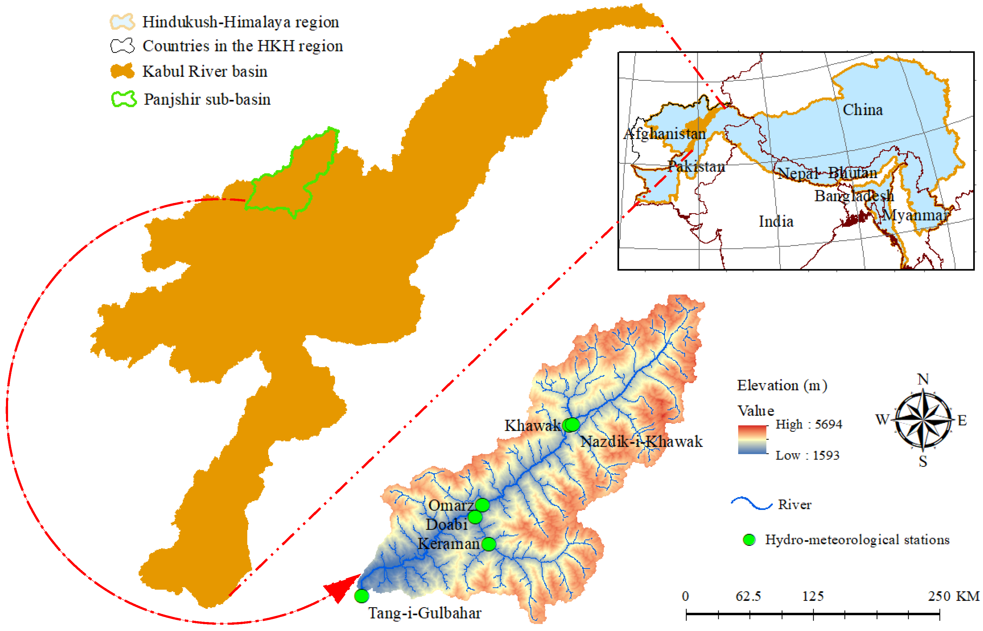
Figure 1. The Panjshir sub-basin of the Kabul River basin and the HKH region.
Hydrology 07 00074 g001
Figure 2. Hypsometric curve of the Panjshir sub-basin, estimated by using ASTER GDEM.
Hydrology 07 00074 g002
Figure 3. Hydro-climatic data in the Panjshir sub-basin.
Hydrology 07 00074 g003
Figure 4. Projected monthly temperature changes during 2040–2060 and 2080–2100: (a) average, (b) lower, and (c) higher under RCP 4.5; and (d) average, (e) lower, and (f) higher under RCP 8.5.
Hydrology 07 00074 g004
Figure 5. Projected monthly precipitation changes during 2040–2060 and 2080–2100: (a) average, (b) lower, and (c) higher under RCP 4.5; and (d) average, (e) lower, and (f) higher under RCP 8.5.
Hydrology 07 00074 g005
Figure 6. Projected SCA during the mid-21st century (2049–2055) under (a) RCP 4.5 and (b) RCP 8.5, in average, lower, and higher temperature and precipitation scenarios.
Hydrology 07 00074 g006
Figure 7. Projected SCA during the late 21st century (2089–2095) under (a) RCP4.5 and (b) RCP8.5, for average, lower, and higher temperature and precipitation scenarios.
Hydrology 07 00074 g007aHydrology 07 00074 g007b
Figure 8. Comparison of the minimum, maximum, and average SCAs projected under RCP 4.5 and 8.5 during the mid- and late 21st century.
Hydrology 07 00074 g008
Figure 9. Projected river flows during the mid-21st century (2049–2055) under (a) RCP 4.5 and (b) RCP 8.5, for the average, lower, and higher temperature and precipitation scenarios and the resulting projected SCAs.
Hydrology 07 00074 g009
Figure 10. Projected river flows during the late 21st century (2089–2095) under (a) RCP4.5 and (b) RCP8.5, for the average, lower, and higher temperature and precipitation scenarios and the resulting projected SCAs.
Hydrology 07 00074 g010
Figure 11. Comparison of projected minimum, maximum, and average discharges during the mid- and late 21st century under RCP 4.5 and 8.5.
Hydrology 07 00074 g011
Figure 12. Streamflow exceedance probabilities in the future relative to the baseline period in the Panjshir sub-basin under three climate change scenarios during the mid-21st century (2049–2055) under (a) RCP 4.5 and (b) RCP 8.5, and during the late-21st century (2089–2095) under (c) RCP 4.5 and (d) RCP 8.5.
Hydrology 07 00074 g012
Table 1. Hydro-meteorological station information used in this study.
Station NameLatitudeLongitudeElevation (m)Data Provided
Tang-i-Gulbahar35.1593277869.288683331625Precipitation, Temperature, Discharge
Omarz35.3758250069.640852782042Precipitation, Temperature
Doabi35.3482972269.618772222059Precipitation, Temperature
Keraman35.2835527869.656927782232Precipitation, Temperature
Khawak35.5648111169.894941672405Precipitation, Temperature
Nazdik-i-Khawak35.5679694469.903908332407Precipitation, Temperature
Table 2. The CMIP5 GCMs used in this study.
IDModelResolutionInstitution
1CMCC-CM0.7° × 0.7°Euro-Mediterranean Center on Climate Change (CMCC), Italy
2CNRM-CM51.4° × 1.4°Centre National de Recherches Météorologiques-Centre Européen de Recherche et de Formation Avancée en Calcul Scientifique (CNRM-CERFACS), France
3CSIRO-Mk3.61.9° × 1.9°CSIRO Marine and Atmospheric Research and the Queensland Climate Change Centre of Excellence (CSIRO-QCCCE), Australia
4GFDL CM32.5° × 2.0°The Geophysical Fluid Dynamics Laboratory in the National Oceanic and Atmospheric Administration (NOAA, GFDL, USA)
5HadGEM2-AO1.9° × 1.2°Institute of Meteorological Research/Korea Meteorological Administration (NIMR-KMA), Korea
6MIROC51.4° × 1.4°Atmosphere and Ocean Research Institute (The University of Tokyo), National Institute for Environmental Studies, and Japan Agency for Marine Earth Science and Technology
(JAMSTEC), Japan
7MPI-ESM-MR1.9° × 1.9°Max Planck Institute for Meteorology (MPI-M), Germany
8MRI-CGCM31.1° × 1.1°Meteorological Research Institute (MRI), Japan
Table 3. Determination of lower and higher temperatures rise under each RCP from the eight GCMs.
GCMsRCP 4.5RCP 8.5
∆T 2040–2060∆T 2080–2100∆T 2040–2060∆T 2080–2100
CMCC-CM1.69 °C2.72 °C3.03 °C6.05 °C
CNRM-CM51.93 °C2.76 °C2.26 °C4.88 °C
CSRIO-Mk3.61.69 °C2.67 °C2.05 °C5.09 °C
GFDL CM31.94 °C4.36 °C2.80 °C7.41 °C
HadGEM2-OA0.69 °C1.68 °C1.06 °C4.09 °C
MIROC51.83 °C2.55 °C2.44 °C5.30 °C
MPI-ESM-MR1.00 °C1.65 °C1.84 °C4.55 °C
MRI-CGCM31.29 °C2.17 °C1.74 °C4.86 °C
Average1.51 °C2.57 °C2.15 °C5.28 °C
Standard deviation0.46 °C0.85 °C0.63 °C1.03 °C
Average − Standard deviation1.04 °C1.72 °C1.53 °C4.25 °C
Average + Standard deviation1.97 °C3.42 °C2.78 °C6.31 °C
Table 4. Determination of lower and higher precipitations changes under each RCP from the selected GCMs.
GCMsRCP 4.5RCP 8.5
∆P 2040–2060∆P 2080–2100∆P 2040–2060∆P 2080–2100
CMCC-CM1.000.971.131.01
CNRM-CM50.940.951.040.88
CSRIO-Mk3.61.051.020.980.84
GFDL CM30.931.071.001.13
HadGEM2-OA0.980.920.870.94
MIROC51.010.991.000.99
MPI-ESM-MR0.901.001.001.14
MRI-CGCM30.940.940.880.89
Average0.970.980.990.98
Standard deviation0.050.050.080.11
Average − Standard deviation0.920.930.900.86
Average + Standard deviation1.021.031.071.09
Table 5. Projected seasonal SCA in (km2) during the mid- and late 21st century under RCP4.5 and RCP8.5, for average, lower, and higher temperature and precipitation scenarios.
SeasonsRCP4.5 Mid-21st CenturyRCP8.5 Mid-21st CenturyRCP4.5 Late-21st CenturyRCP8.5 Late-21st Century
Average temperature and precipitation
Autumn−85−108−229−577
Winter−69−121−187−575
Spring−242−426−495−1117
Summer−131−186−205−256
Higher temperature and lower precipitation
Autumn−249−406−317−815
Winter−35−113−198−859
Spring−156−381−642−1299
Summer−164−227−226−257
Lower temperature and higher precipitation
Autumn108−5367−348
Winter3−128−112−309
Spring−60−435−269−614
Summer−61−151−147−242
Table 6. Projected seasonal flows variations in m3/sec during the mid- and late 21st century under RCP4.5 and RCP8.5, for average, lower, and higher temperature and precipitation scenarios.
SeasonsRCP4.5 Mid-21st CenturyRCP8.5 Mid-21st CenturyRCP4.5 Late-21st CenturyRCP8.5 Late-21st Century
Average temperature and precipitation
Autumn−5−7−8−8
Winter−2−3−3−0.2
Spring20255−20
Summer−30−49−57−81
Higher temperature and lower precipitation
Autumn−7−8−9−8
Winter−3−4−31
Spring26183−49
Summer−32−60−70−83
Lower temperature and higher precipitation
Autumn−1−6−7−8
Winter−1−1−3−1
Spring3123248
Summer−5−38−39−71