Abstract
On many tropical reefs, submarine groundwater discharge (SGD) provides a substantial and often overlooked nutrient source to nearshore ecosystems, yet little is known about the impacts of SGD on the biology of reef organisms. To address this, the physiological responses of the endemic rhodophyte Gracilaria coronopifolia and an invasive congener, Gracilaria salicornia, were examined across an SGD gradient in the field and laboratory. Tissue samples of both species were cultured for 16 days along an onshore-offshore SGD gradient at Wailupe, Oahu. G. salicornia tolerated the extremely variable salinity, temperature, and nutrient levels associated with SGD. In marked contrast, half of G. coronopifolia plants suffered tissue loss and even death at SGD-rich locations in the field and in laboratory treatments simulating high SGD flux. Measurements of growth, photosynthesis, and branch development via two novel metrics indicated that the 27‰ simulated-SGD treatment provided optimal conditions for the apparently less tolerant G. coronopifolia in the laboratory. Benthic community analyses revealed that G. salicornia dominated the nearshore reef exposed to SGD compared with the offshore reef, which had a greater diversity of native algae. Ultimately, SGD inputs to coastal environments likely influence benthic community structure and zonation on otherwise oligotrophic reefs.
Keywords:
Gracilaria; algae; groundwater; invasive; reef ecology; nutrients; SGD; photosynthesis; salinity; benthic 1. Introduction
Terrestrial groundwater may discharge directly to the marine environment wherever a coastal aquifer is connected to the sea [1]. It is generally understood that this process of submarine groundwater discharge (SGD) is a significant source of nutrients, carbon, and metals to coastal waters worldwide [1,2,3,4,5]. Although the quality and quantity of groundwater input to marine environments have been well documented, the effects of SGD on biological processes remain understudied [6]. These effects may be amplified in tropical, oligotrophic environments where primary productivity is typically limited by low nutrient levels in coastal waters [7,8,9]. In tropical and sub-tropical regions, the influx of terrestrial groundwater to the marine environment typically results in increased nutrient concentrations and decreased temperature and salinity of nearshore waters compared with ambient oceanic conditions [10,11,12,13,14], and these changes relax the nutrient limitations typical of coral reefs. Even small additions of nutrients to oligotrophic waters can increase primary productivity in marine algae [15]. Increases in algal growth rate, photosynthetic rate, and tissue nitrogen (N) are often observed as nutrient concentrations increase [15,16,17].
Groundwater enriched with anthropogenically derived nutrients has been implicated in the development of harmful algal blooms [2,18] and ecosystem changes associated with eutrophication [19,20]. SGD increased primary production and played a role in the shift from seagrass-dominated (Thalassia testudinum) cover to green filamentous algae at sites near the Yucatan Peninsula [21]. Elevated δ15N values in the tissue of several marine algae suggest that terrestrially derived nutrients, which are transported via SGD, are likely to play an important role in the supporting algal blooms in Hawaii [17,22].
In addition to nutrient flux, variation in nearshore salinity associated with SGD may also impact primary productivity. Salinity effects are well-recognized factors affecting the growth rate, development, and distribution of marine plants [23,24,25]. Maximal growth rates and photosynthetic response of some tropical reef algae, including species of Gracilaria, were reported for samples incubated in hyposaline, nutrient-rich waters [24,26]. Species that have high nutrient uptake rates and a wide tolerance to reduced salinities are likely to have a competitive advantage in regions with tidally modulated, hyposaline groundwater flux.
In Hawaii, Gracilaria salicornia (C. Ag) E. Y. Dawson is considered an invasive species with the competitive ability to exclude other benthic organisms [27]. It is hypothesized that this alga arrived in Hilo, Hawaii, as part of solid ballast of one or more sailing ships from the western tropical Pacific. G. salicornia was intentionally introduced to Oahu in the 1970s from this known population on Hawaii Island for experimental aquaculture [27]. After that introduction into the waters of Waikīkī and Kāneʻohe Bay, this species eventually dominated the benthic environments in these areas, with new populations observed on multiple Oahu reefs [27]. The competitive success of this species has been attributed to its ability to create a mat-forming morphology (up to 10 cm thick), in addition to its ability to tolerate large variations in salinity, temperature, and desiccation [27]. In addition to direct competition with corals [28], G. salicornia occupies habitats that would normally support endemic species, such as the congener Gracilaria coronopifolia (J. Ag) [29]. Although G. coronopifolia was one of the three most common seaweeds used for food and one of the 10 most common intertidal species in the recent past, this endemic is now much less abundant due to overharvesting and likely competitive pressure from G. salicornia and other invasive algae [30,31].
To better understand abiotic drivers that influence the competitive successes of benthic algae, the physiological effects of SGD on G. coronopifolia were compared with those of G. salicornia across a highly variable onshore-offshore gradient of SGD in the field. Further, the response of the apparently vulnerable G. coronopifolia to various levels of simulated SGD was measured in a controlled laboratory setting. The results of this work suggest that exposure to SGD can increase the growth rate, photosynthetic performance, branch development, and tissue N% of G. salicornia samples when compared to samples with no SGD exposure. More importantly, these data suggest that SGD can play a strong role in limiting a native, such as G. coronopifolia, from seep regions. Finally, this study suggests that SGD input to coastal environments may more broadly influence benthic community structure and zonation on otherwise oligotrophic reefs.
2. Materials and Methods
2.1. Field Experiment: Wailupe Reef
Wailupe Reef (Figure 1) is a well-studied coastal site characterized by an onshore-offshore gradient of nutrients and salinity that is similar to other coastal areas in Hawaii with relatively high SGD flux [10,17,32,33]. Previous studies at this site report estimated discharge rates of 30,000 m3 d−1 using seepage meters [34] and from 13,000 m3 d−1 [35] to 95,490 m3 d−1 [36] using a 222Rn mass balance assessment. SGD at Wailupe flows from distinct springs and porous sediments to the water column [35,37]. Although residence time estimates for SGD at this location (2.5–5.5 days) indicate SGD-derived nutrients may be available for reef plants for many days, SGD flux and nutrient concentrations in the water column can be greatly reduced during high tide [35,36]. The benthic habitat at Wailupe Beach Park has been characterized as a shallow reef flat consisting of sand, pavement, and aggregate reef that is dominated by macroalgae with 10–90% cover (NOAA Shallow-Water Benthic Habitats: Insular Pacific; https://www.ngdc.noaa.gov/). The objective of this field experiment was to compare the physiological response of two algal congeners at three locations across a previously described SGD gradient at Wailupe Reef.
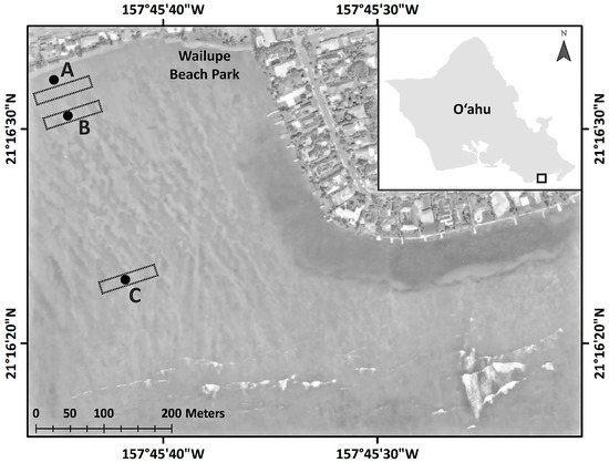
Figure 1.
Study locations at Wailupe Reef. Experimental locations A, B, and C are shown as black dots identified by boldface letters overlain on an aerial image (ESRI Basemaps). The approximate locations of benthic surveys are shown by dashed rectangles.
2.1.1. Sample Selection, Pretreatment, and Initial Measurements
Individual plants of G. coronopifolia (Hawaiian endemic) and G. salicornia (C. Ag.) (invasive) were collected from a single location, at a shallow nearshore reef in southern Oahu at Ala Moana Beach Park, on 19 April 2014. At the University of Hawaii at Mānoa (UHM), these plants were then acclimated to low-nutrient, artificial seawater (distilled water + Instant Ocean® Sea Salt) for 10 days to draw down internal N storage following Amato et al. (2016). These plants were placed in two separate 75-l aquaria with aeration under 200 µmol photon m−2 s−1 PAR µmol cool-white fluorescent light, as measured by a 4π Li-Cor® quantum sensor (model LI-193SA, Li-Cor, Lincoln, NE, USA), for 12 h day−1 at 23 °C. Every two days, reagent grade nitrate (NaNO3) and phosphate (NaH2PO4) were added with distilled water to maintain the water nutrient and salinity levels typical of oligotrophic coastal waters in Hawaii: 0.2 µM NO3−, 0.05 µM PO43− at 35‰ salinity [10]. Salinity was measured with a YSI conductivity meter (model EC300, Yellow Springs Instruments, Yellow Springs, OH, USA). At the end of this pretreatment, three samples of each species were then triple-rinsed in distilled water, dried at 60 °C until a constant mass was achieved, ground to powder, and submitted to the Biogeochemical Stable Isotope Facility (BSIF) at UHM for the analysis of tissue δ15N, N%, and C%. Ratios of 15N:14N were expressed as δ15N (1), in which Rstandard is relative to atmospheric N2 [38].
Tip Score (TS), a novel morphological index, aided sample selection based on an assessment of plant wet mass (Sartorius balance model A200S, Sartorius, Bohemia, NY, USA) and enumeration of apical tips for each plant. This approach was developed to minimize morphological variability among samples (2).
On day 0, 18 samples of each species showing no sign of reproductive or necrotic tissue were selected for field deployment according to the following criteria: 50 < TS < 100 for G. coronopifolia and 10 < TS < 20 for G. salicornia. Differences in these initial TS value ranges were necessary because of natural differences in axis diameter (and mass to tip # ratio) between these species.
Rapid Light Curves (RLC) were performed on six samples of each species as a measure of initial photosynthetic performance using Junior-PAM (Walz, Effeltrich, Germany) set to default values. The RLC was used to estimate the sample’s electron transport rate (ETR) at various levels of irradiance. Samples were placed within a magnetized clip just below a dichotomous branch. All RLCs were performed using actinic photosynthetically active radiation (PAR) intensities of 0, 66, 90, 125, 190, 285, 420, 625, and 820 µmol photons m−1 s−1 produced using a blue light-emitting diode (LED). Three parameters—maximum electron transport rate (ETRmax), low-light efficiency (alpha), and minimum saturating irradiance (Ek)—were generated using WinControl-3 (Walz, Germany) software version 3.23. Alpha is a measure of the efficiency of light harvesting and equal to the slope of the RLC in the light-limited region of an RLC. Ek is the irradiance value at which alpha intercepts ETRmax and is considered the irradiance at which photosynthesis reaches its steady state rate [39].
2.1.2. Sample and Data Logger Deployment
Three locations with a similar depth (~0.5 m deep at 0.0 m above sea level) were chosen along an onshore-offshore gradient of SGD on the Wailupe reef flat (Figure 1). Location A was centered on a prominent submarine groundwater spring, approximately 25 m from shore, that was previously characterized [36]. Location B was approximately 81 m from shore and had no detectable spring influence. Location C, approximately 337 m from shore, was presumed to be relatively unimpacted by SGD, as judged from preliminary measurements of salinity at low tide (data not shown); this offshore location was 0.20 m deeper than locations A and B. At each location, six replicate sites were oriented in a hexagonal pattern, with 2 m between adjacent sites.
On 29 April 2014, individual algal samples were randomly assigned to field sites before being placed in cylindrical cages (20 × 8 cm) made of plastic mesh covered with polyester mesh fabric (8 mm diameter) that allowed water to flow but prevented samples from being subjected to grazing by local reef herbivores. At each site, one cage containing a single G. coronopifolia sample and one cage containing a single G. salicornia were suspended in tandem 0.25 m below the water surface on a single line tethered to a cinderblock anchor and small float.
Specific conductances and temperatures of surrounding waters were monitored at the bottom of a single algal cage every minute for a full tidal cycle on days 0, 6, and 15 with a data logger (CTD-Diver Model DI272, Schlumberger, Houston, TX, USA) at all locations. Salinity (‰) was calculated from CTD-Diver data using conductivity normalized to 25 °C. One HOBO data logger (model UA-002-64, Onset Computer Corporation, Bourne, MA, USA) was attached to a cage at each location to record the temperature from days 6 through 16. Water samples were collected at the center of each location at a water level equal to the middle of the algal cages on days 7, 15, and 16 at different tidal heights, filtered (0.45 µm) into acid-washed 60 mL bottles, and submitted to SOEST Laboratory for Analytical Biogeochemistry (SLAB) at UHM for analysis of nitrate + nitrite (NO3− + NO2−), phosphate (PO43−), silicate (SiO42−), and ammonium (NH4+). Duplicate water samples (n = 3 duplicate pairs) were submitted to estimate analytical error, which was calculated as the average error between duplicates (the absolute value of the difference between duplicate samples expressed as a percentage of the mean of duplicate sample values). During water sample collection, the salinity of the water column was measured with a YSI meter at each location. If stratification was observed, additional water samples were collected within each stratum. Nutrient results were pooled with data from samples collected in 2010 [36] at similar locations to determine the relationship between nutrients and salinity. Tidal measurements (water height) were obtained from the Honolulu observation station # 1612340 located in Honolulu Harbor (National Oceanic and Atmospheric Administration 2014).
Sample cages were collected at 13:00 on day 16 from all sites, placed in 20 L buckets of water from each location, and held in the sun under 50% shade cloth on land. RLCs were quickly performed on samples to assess photosynthetic performance (as above). All samples were then placed in seawater (34.9‰ salinity) for 3 h to control for osmotic mass effects before the final wet mass was determined at UHM (as above), and the number of live (absence of necrotic or bleached tissues) apical tips of each sample was recorded. All sample tissues were then prepared for the analysis of δ15N, N%, and C% at BSIF (as above). A subset of duplicate tissue samples (n = four duplicate pairs) was submitted to BSIF to estimate analytical error (as above). A final TS value was calculated for each location using Equation (2). The growth rate of each sample was calculated as the percent change in wet mass per day using Equation (3). To quantify changes in the number of apical tips, the parameter “Tip Index” (TI) was developed, as shown in Equation (4).
2.1.3. Benthic Community Assessment
The benthic community at each location was analyzed using a Nikon AW110 camera attached to a PVC photoquadrat frame (18.2 × 27.0 cm) on 18 March 2014, following a modified CRAMP rapid assessment protocol [40] as described in [17]. Five transect locations were randomly chosen within a 4 × 100 m area, using ArcMap Desktop 10.0 (ESRI, Redlands, CA, USA), at each study location (Figure 1). One photograph (representing 458.8 cm2 of reef) was taken every meter along each 10 m transect. The percent cover of benthic organisms or abiotic substrate was estimated with PhotoGrid [41] software using a point intercept method and 25 random points per image. Macroalgae were identified to the species level where possible, and other organisms were grouped into functional groups, such as turf algae, crustose coralline algae (CCA), coral, and zoanthids. The Shannon Diversity Index Equation [42] and the Simpson Dominance Index Equation (6) [43] were calculated for each transect as:
SigmaPlot 11 (Systat software Inc., San Jose, CA, USA) was used to perform all statistical tests. If parameter data were normal and homoscedastic, one-way Fisher ANOVA tests (shown as F statistic) and Tukey pairwise comparisons were used to compare the mean of sample values among locations. If either of these assumptions were violated, the non-parametric, one-way Kruskal–Wallis ANOVA test (shown as H statistic) was calculated and the Student–Newman–Keuls Method was used for pairwise comparisons.
2.2. Simulated SGD Study
The objective of this laboratory experiment was to compare the physiological response of the apparently less tolerant G. coronopifolia to treatments that simulate various amounts of SGD in a highly controlled mesocosm. Fifty G. coronopifolia individuals were collected on 19 October 2007 and 11 October 2008 at Ala Moana Beach Park, Oahu, for two replicate experiments at UHM.
2.2.1. Sample Selection, Pretreatment, Mesocosm Design, and Initial Measurements
One axis was cut from each individual and placed in a 3 L beaker with nutrient and salinity levels typical of oligotrophic coastal waters [10] in Hawaii to acclimate (as above). The beaker was then placed in a growth chamber (Environmental Growth Chambers, model GC-15, Chagrin Falls, OH, USA) at a temperature of 25 ± 0.5 °C for 10 days with aeration. Irradiance was set to 250 µmol photons m−2 s−1 PAR via high-output cool-white fluorescent bulbs, as measured by a calibrated 4π Li-Cor quantum sensor, for 12 h day−1.
For each 16-day replicate trial, a unidirectional flow-through mesocosm supported four treatments of six samples. Treatment water was pumped at a constant rate of 1.6 L day−1 from four 200 L HDPE drums into 24 × 800 mL glass beakers using a digital peristaltic pump. Beakers were aerated and located in one of two water baths. Excess treatment water continuously flowed from the beakers to the water bath and then exited the mesocosm via a hose located 10 cm above the bottom of the bath.
The experimental concentrations of nitrate and phosphate were set for each treatment via published relationships derived from SGD studies in Hawaii [10]. Four salinity levels were chosen to simulate varied amounts of SGD, and the associated nutrient concentrations were calculated using the following equations: [NO3−] = −3.3 × salinity + 115.7 and [PO43−] = −0.14 × salinity + 4.9 [10]. Distilled water was mixed with Instant Ocean® Sea Salt and reagent grade nutrients (NaNO3 and NaPO4) to produce the following four treatments, hereafter referred to by their salinity value: (A) 35‰ salinity + (0.20 µM NO3−, 0.05 µM PO43−); (B) 27‰ salinity + (7.51 µM NO3−, 0.15 µM PO43−); (C) 19‰ salinity + (23.36 µM NO3−, 1.65 µM PO43−); (D) 11‰ salinity + (82.68 µM NO3−, 3.75 µM PO43−). To minimize immediate P limitation in the 35‰ SGD treatment (the PO43− equation produced a result of zero when solved for a salinity of 35‰), a PO43− concentration of 0.05 µM PO43− was used in this treatment. This low level of P is within the range of dissolved reactive P reported for oceanic waters near Hawaii [44].
Twenty-four samples showing no sign of reproductive or necrotic tissue were selected, as above, using the following criteria: 50 < TS < 100. After initial processing, all samples were randomly assigned to a single treatment beaker in the growth chamber. Every 4 days, samples were removed from the growth chamber and placed on a shaker table in treatment water under cool-white fluorescent light at 50 µmol photons m−2 s−1 PAR for data collection.
2.2.2. Data Collection
On days 0, 4, 8, 12, and 16, the wet mass and apical tip number of all samples were recorded as above. RLCs were performed on days 0, 8, and 16 for all samples in treatment water between 12:00 and 14:00; a Diving-PAM (Walz Co., Effeltrich, Germany) with a blue actinic beam and a 5.5 mm active diameter fiber optic cable was used to perform RLCs. Only the RLC results from Trial 2 are reported in this study because unexpectedly high within-treatment variability during the first replicate trial necessitated the use of a modified tissue holder (a rubber cap with a 1 × 2 mm slot) for the fiber optic cable of the Diving-PAM. Raw Diving-PAM data were imported using WinControl software (Walz GmbH, Effeltrich, Germany). RLC parameters (as above, ETRmax, alpha, and Ek,) were calculated by nonlinear regression using SigmaPlot 11 software.
The final values (day 16) of TS, growth rate, and TI were calculated for each sample. Fisher’s one-way ANOVA test (shown as F statistic) and Tukey pairwise comparisons were conducted using SPSS software (SPSS Inc., Chicago, IL, USA) if the distribution of parameter data was normal and homoscedastic. Welch’s ANOVA test (shown as Fw statistic) and Games-Howell pairwise comparisons were performed using SPSS software if the distribution of parameter data was normal and heteroscedastic. A non-parametric one-way Kruskal–Wallis ANOVA test (shown as H statistic), Tukey pairwise comparisons, and Spearman’s rank order correlations (shown as rs statistic) were performed with SigmaPlot 11 if the assumption of normality was violated.
3. Results
3.1. Wailupe Reef Study
3.1.1. Physical Conditions at Wailupe Reef
The water column at Wailupe Reef appeared to be well mixed, as salinity was generally consistent with depth at the time of water sample collection. During the 16-day deployment at Wailupe Reef, salinity, temperature, and dissolved nutrient concentrations varied widely onshore at location A and nearshore at location B. Figure 2 shows salinity, water level, and modeled nutrient concentrations for the water column at Wailupe during two spring tidal cycles (29–30 April and 14–15 May) and one neap tidal cycle (5–6 May) in 2014. The greatest variability in salinity and temperature was observed at location A with a minimum of 2.4‰ (Figure 2a) and 22.0 °C (Figure S1). In contrast, salinity (Figure 2a) and temperature (Figure S1) were the least variable at location C, where salinity was not influenced by water height (Figure 2a). One exception was an extremely low tide event (15 May) at location B, where two distinct layers of water were observed. At this time, surface water had a salinity of 11‰ (sample Wailupe B LowLow1; Table A2), whereas the salinity next to the algal cages near the benthic surface was 24‰ (sample Wailupe B LowLow2; Table A2). This may be attributable to the diffuse nature of SGD seepage at this location as compared with location A, which visibly showed a high rate of point source discharge (surface of water appeared to boil, and sand was forcefully suspended in the water column) from a prominent spring.
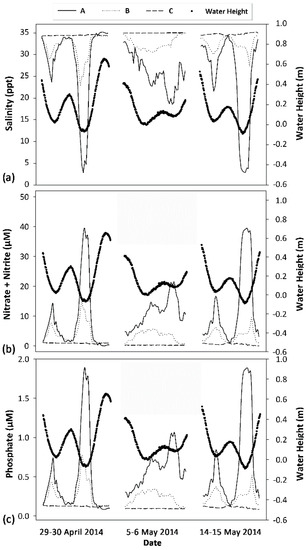
Figure 2.
Time series results for salinity, water height, and nutrients at Wailupe Reef study locations. (a) Salinity (primary y-axis) vs. date; (b) estimated dissolved NO3− + NO2− (primary y-axis) vs. date; and (c) estimated dissolved PO43− (primary y-axis) vs. date. Water height (secondary y-axis) is shown as large dots for all plots. Locations A, B, and C are shown as solid lines, dotted lines, and dashed lines, respectively.
Nutrient concentrations at Wailupe were modeled over time using linear equations calculated from water sample data for NO3− + NO2− (NO3− + NO2− (µM) = 42.858 − (1.220 × salinity) r2 = 0.930) and PO43− (PO43− (µM) = 2.045 − (0.0558 × salinity) r2 = 0.968). Using these relationships and time-series measurements of salinity, NO3− + NO2− and PO43− concentrations were estimated at all locations for three different days (Figure 2b,c). Maximum concentrations of NO3− + NO2− (42.70 µM), PO43− (1.95 µM), and SiO42− (668.8 µM) were measured at location A (sample A-LL; Table A2) when water height reached a minimal value of −0.1 m. Elevated concentrations of NO3− + NO2− and PO43− persisted for most of the day at locations A and B (Figure 2b,c) relative to location C. The highest daily NO3− + NO2− and PO43− concentrations were observed when water height reached the lowest values (Figure 2b,c). When tidal exchange was relatively minimal (neap tide), NO3− + NO2− and PO43− did not approach the minimum concentrations shown during the lower-high tide as observed during spring tides (Figure 2b,c). In contrast, nutrient levels offshore at location C remained low and did not appear to vary with changes in water height (Figure 2). The mean error of duplicate nutrient samples was 1.4%, 5.4%, 1.0%, and 4.1% for PO43−, SiO42−, NO3− + NO2−, and NH4+, respectively.
A very strong onshore-offshore gradient occurred at Wailupe Reef, exhibiting high levels of SGD at location A and moderate levels of SGD at location B relative to the offshore location C. At nearshore locations, SGD flux was associated with large variations in salinity, nutrients, and temperature, particularly at location A, which was adjacent to a discrete submarine spring. The offshore location C did not appear to be influenced by SGD during this study. Differences in maximal water height and associated nutrient concentrations between spring and neap tides suggest that nearshore locations on Wailupe Reef experience consistently elevated nutrient levels during neap tides but not spring tides.
3.1.2. Physiological Response of Deployed Algae
An onshore-offshore gradient in algal tissue N% was observed for both species across locations (Table 1). Significant differences in mean tissue N% were detected among locations in G. coronopifolia (F = 23.189, p < 0.001) and G. salicornia (F = 23.725, p < 0.001). Pairwise comparisons indicate that the mean values of tissue N% in both species were greater in samples from location A compared with location C (Table 1). For both species tested, the initial values of mean tissue N% (Table A1) were substantially lower than the final values of samples deployed at location A, and similar to final values from samples deployed at locations B and C (Table 1). Therefore, algal tissue N only increased during this study at location A.

Table 1.
Final algal tissue N and C parameter values for Gracilaria coronopifolia and Gracilaria salicornia deployed at three locations at Wailupe reef. Mean values (mean ± SD) are shown for tissue δ15N‰, N%, C%, and C:N for both species by location. Boldface letters indicate the results of pairwise comparisons among locations for each species separately; locations that share a common letter are not significantly different (p < 0.05). Sample size (n) indicates the number of samples recovered on day 16.
Onshore-offshore trends in tissue C:N and δ15N values were found for both species (Table 1). Significant differences among locations were detected for tissue C:N values in G. coronopifolia (H = 8.695, p = 0.004) and G. salicornia (F = 17.260, p < 0.001). Final tissue δ15N values were approximately 2.5‰ higher at locations A and B compared with C in both species (Table 1); significant differences among locations were detected for tissue δ15N values in G. coronopifolia (F = 69.743, p < 0.001) and G. salicornia (H = 11.463, p = 0.003). Final tissue δ15N values from samples deployed at locations A and B (Table 1) were greater than initial values in both species (Table A1). Mean analytical errors of duplicate tissue samples were 1.2%, 13%, and 22.8% for δ15N, N%, and C%, respectively. Increases in tissue δ15N over time at locations A and B suggest the uptake of a terrestrial-based N source with a higher δ15N value than that of the offshore water at location C.
Measured differences in photosynthetic parameters indicate that the maximum photosynthetic rate (ETRmax) and photosynthetic efficiency at low light (alpha) were greater at nearshore locations with SGD relative to the offshore location C in G. salicornia samples. Mean ETRmax values were greatest for G. salicornia tissues deployed at location B (40.4 ± 8.8 μmol e− m−2 s−1; Table 2). ANOVA tests detected significant differences among treatments for G. salicornia samples (H = 11.099, p = 0.004); pairwise comparisons indicate samples at locations A and B had higher mean values for ETRmax than location C but were not different from each other (Table 2). An identical result was found for values of alpha (F = 12.367, p < 0.001); pairwise comparisons were significant for both locations A and B vs. C. G. salicornia samples deployed at location A had more new branch development than samples at the offshore location C; ANOVA tests indicate differences in mean TS (F = 6.640, p = 0.009) and TI values (H = 10.561, p = 0.005). Post hoc comparisons show G. salicornia samples at location A had greater mean TI and TS values compared with the offshore location C (Table 2). Despite the increased photosynthetic response and branching of G. salicornia samples at SGD-influenced locations, large variability in growth rate was found among and within locations (Table 2), and no significant differences were detected (H = 1.556, p = 0.459, n = 18). A similar result was found for growth rates of G. coronopifolia samples among locations (H = 2.074, p = 0.381, n = 14). See Figure S2 for photographs of apical tip development in representative samples of both species.
Table 2.
Final values of growth rate, Tip Score (TS), Tip Index (TI), and PAM parameters for both field and laboratory studies. Gc = G. coronopifolia and Gs = G. salicornia. Values (mean ± SD) are shown for growth rate, TS, TI, maximum electron transport rate (ETRmax), low-light efficiency (alpha), and minimum saturating irradiance (Ek) for all treatments (or locations). Sample size (n) is shown for each treatment. Units for growth rate, ETRmax, alpha, and Ek are: % day−1, µmol e− m−2 s−1, µmol photon m−2 s−1 photosynthetically active radiation (PAR), and (µmol e− m−2 s−1) (µmol photon m−2 s−1)−1, respectively. Tip Score and Tip Index are unitless. Boldface letters indicate the results of pairwise comparisons among locations tested for each species separately: locations that share a common letter are not significantly different (p < 0.05).
The routine measurement and observation of deployed algal samples revealed that G. coronopifolia tissues were particularly intolerant of locations with high SGD flux. G. coronopifolia tissues at locations A and B showed signs of pigment loss and tissue necrosis after eight days. By the end of the study, three of six G. coronopifolia samples at location A and one of six G. coronopifolia samples at location B were not recovered and presumed dead (Table 2). Figure S3a,b show the initial and final photographs of a single G. coronopifolia sample that was deployed at location A as an example of pigment loss and tissue necrosis in this species. The loss of G. coronopifolia samples alongside high intralocation-variability likely contributed to a lack of power to identify statistical differences in growth rate, branching, or photosynthetic parameters, except for Ek: (F = 4.804, p = 0.032). Because of the differences in the initial parameter values in addition to sample loss, statistical comparisons between the two species were not attempted. Surprisingly, G. salicornia samples also showed signs of intolerance to conditions at the offshore location C after 12 days, and negative values for the final mean growth rate and mean TI were calculated at this location (Table 2). Figure S3c,d illustrate that some samples of G. salicornia deployed under low-nutrient conditions at location C experienced pigment loss and tissue necrosis similar to that seen in some G. coronopifolia samples exposed to high SGD flux.
Using pooled data from all locations, branch development showed significant relationships with both growth rate and tissue N%. A positive non-linear relationship was detected between growth rate and TI: Growth Rate = a × (1 − bTI) for both G. salicornia (r2 = 0.65, p < 0.0001) and G. coronopifolia (r2 = 0.78, p < 0.0001. This suggests that Gracilaria plants that have more branches may gain mass faster than those that have fewer branches. Tissue N% was also positively related to TS (r2 = 0.645, p < 0.001) and TI (r2 = 0.350, p = 0.010) in G. salicornia across all locations.
3.1.3. Benthic Community Assessment of Wailupe Reef
Invasive G. salicornia and Acanthophora spicifera, as well as the native species Spyridia filamentosa, Halimeda spp., and Galaxaura rugosa, represented the extent of macroalgal species in benthic transects at Wailupe (Figure 3). Although all locations had a similar proportion of macroalgae (Table 3), G. salicornia dominated the benthic environment at SGD-influenced locations A and B (Figure 3). In contrast, location C had the greatest mean diversity of benthic organisms (Table 3), a significantly lower proportion of invasive macroalgae (H = 11.580, p = 0.003), and a significantly greater proportion of native macroalgae (H = 11.618, p = 0.003). At this offshore location, native macroalgae S. filamentosa and Halimeda spp. were the most abundant, and G. salicornia represented less than 10% of these transects (Figure 3). Interestingly, location B had the highest proportion of G. salicornia (Figure 3) and the lowest diversity (Simpsons Index; F = 8.802, p = 0.004) and highest dominance (Shannon’s Index; F = 7.109, p = 0.009) values (Table 3).
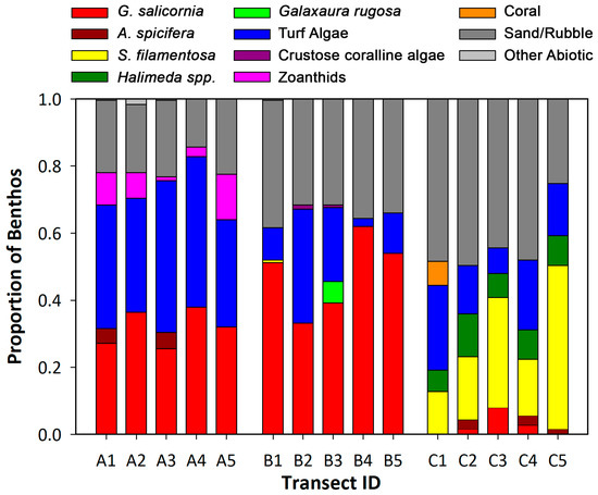
Figure 3.
Benthic cover analysis for Wailupe Reef transects. The proportion of benthic cover for each transect at Wailupe Reef.
Table 3.
Average percent cover (mean ± SD) of benthic organisms and diversity indices by location. Crustose coralline algae are represented by crustose coralline algae (CCA). Sand, gravel, and coral rubble are represented by % Abiotic. The Shannon Diversity Index and the Simpson Dominance Index are shown as H’ and λ’, respectively. Boldface letters indicate the results of pairwise comparisons among locations for each species separately: locations that share a common letter are not significantly different (p < 0.05).
3.2. Simulated SGD Study
3.2.1. Growth Rate and Branch Development: Pooled Trials
The results of two replicate trials were pooled to calculate the growth rate and changes in apical tip number in G. coronopifolia samples over 16 days. Samples exposed to the treatment representing a relatively moderate flux of SGD (27‰) had greater growth rates and branch development than treatments with high SGD flux (11‰) and no SGD flux (35‰). A maximum mean growth rate of 3.0 ± 0.6% day−1 was observed for plants in the 27‰ treatment (Table 2), that was significantly higher than all other simulated SGD treatments (Fw = 30.827, p = 0.000). Pairwise comparisons showed that the growth rate of samples in the 19‰ treatment (2.2 ± 0.5% day−1) was greater than that in the 35‰ treatment (1.1% day−1 ± 0.4; Table 2). Samples exposed to the treatment with the lowest salinity (11‰) had the lowest mean growth rate (1.4% day−1 ± 1.5) and the highest variability (Table 2). Nearly half of the G. coronopifolia samples in this treatment had evidence of pigment loss and necrotic tissue within the first four days of each replicate trial. This result is very similar to the field observations for this species deployed at SGD-influenced locations on Wailupe Reef.
G. coronopifolia samples subjected to the 27‰ SGD treatment had the highest mean value among treatments for TI (132.7 ± 105.8; Table 2). Significant differences were detected for mean TI values among treatments (H = 32.720, p < 0.001), and pairwise comparisons showed that plants in the 27‰ treatment had higher TI values than the 35‰ and 11‰ treatments (Table 2). Similar to the field study on Wailupe Reef, a positive correlation was found between growth rate and TI (rs = 0.59, p = 0.000), suggesting that the rate of branch development is closely tied with the growth rate of this alga.
3.2.2. Photosynthetic Response: Replicate Trial 2
Measurements of photosynthetic response in G. coronopifolia samples indicated that the 27‰ SGD treatment provided the most conducive conditions to photosynthesis of all four treatments tested. Plants subjected to the 27‰ treatment had the greatest mean values for all photosynthetic parameters (Table 2), as calculated for each sample by non-linear regression (all r2 > 0.99), on day 16. Significant differences were detected among SGD treatments for values of ETRmax (F = 25.73, p = 0.000) and Ek (F = 25.48, p = 0.000), but not alpha (F = 2.601, p = 0.081). Samples in the 27‰ treatment had significantly greater mean values for ETRmax (44.7 ± 8.1 µmol e− m−2 s−1; p < 0.01) and Ek (163.0 ± 27.9 µmol photon m−2 s−1 PAR; p < 0.05) relative to the other treatments. A representative mean RLC was calculated for each treatment using the average ETR value of samples at a given irradiance (r2 > 0.99 for all treatments). Not surprisingly, plants in the 27‰ treatment had a greater mean photosynthetic rate at nearly every irradiance level than the other treatments (Figure 4).
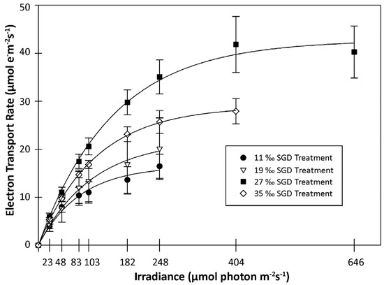
Figure 4.
Rapid light curves for Gracilaria coronopifolia in the simulated submarine groundwater discharge (SGD) experiment. The electron transport rate (mean ± SD) for each treatment at a given irradiance is shown. Non-linear regression lines (solid lines) were fit to the mean value at a given irradiance for each treatment.
4. Discussion
Recent estimates of SGD flux to coastal environments suggest that SGD provides a similar or greater amount of freshwater and terrestrial nutrients to coastal oceans than riverine inputs on a global scale [2,3,5,14,45]. Using 228Ra, a recent study found that Indo-Pacific Oceans receive nearly 70% of global SGD flux [5]. Located near the center of the Pacific Ocean, Hawaii has become a hotspot for SGD investigations in recent decades because its highly elevated islands offer large hydraulic gradients, which, in combination with a permeable volcanic substrate, can result in relatively high SGD flux rates and associated solute input to coastal waters [14]. Although SGD research in Hawaii and around the world has shown that SGD commonly occurs over large special scales and occurs with highly variable rates of flow [3,10,12,14,33,35,46], we are only beginning to understand the impacts of this process on marine ecosystems and biota [6]. In this study, changes in nearshore water quality associated with SGD flux were found to influence significant physiological responses, such as growth rate, photosynthetic performance, tissue nutrient content, and branch development, of two closely related macroalgae. More importantly, SGD flux appeared to influence benthic community structure on a shallow Hawaiian reef by promoting the growth and persistence of invasive species adapted to hyposaline conditions, while extreme SGD appeared to limit the distribution of a less tolerant native species.
4.1. Physiological Responses of Gracilaria to SGD
Irradiance, osmotic forces, temperature, and nutrient availability are important abiotic factors that influence the growth, distribution, and reproduction of primary producers. The results of the experiments in the field and lab suggest that variations in salinity–nutrient combinations associated with SGD flux are very strong factors influencing the growth, persistence, and competitive success of the Gracilaria species examined in this study. The relative ecological success of G. salicornia compared with G. coronopifolia is consistent with G. salicornia’s wide tolerance to low salinity and high temperature. This was expected, as a previous study found that G. salicornia maintained high growth rates when cultured in freshwater for 1 week [27]. In contrast, G. coronopifolia showed signs of osmotic stress when subjected high levels of SGD flux. This stress manifested in tissue loss (including apical tips) and, ultimately, the loss of entire samples in both the field and a highly controlled laboratory setting.
The maintenance of positive growth despite osmotically induced stress may be more important to a plant’s competitive success than its rate of growth in some locations. As a euryhaline genus, many species of Gracilaria have maximal growth rates at salinities from 15‰ to 30‰ [26,47,48]. Although differences in growth rate were not found among locations in either species at Wailupe, it is clear that both species acquired significantly more terrestrial-N at location A compared with the other locations. Increased tissue N is likely to have played a role in the optimization of photosynthetic performance in the salinity-tolerant G. salicornia at location A. Higher ETRmax values at location A compared with the offshore location C suggest that SGD-N subsidies relaxed nutrient limitation and enhanced the photosynthetic capacity of on-shore plants. Similar results were found for other bloom-forming macroalgae in Hawaii; increased nutrient availability led to increased tissue N%, growth rate, and ETRmax values in Ulva lactuca, Acanthophora spicifera, and Hypnea musciformis under controlled conditions [15]. ETRmax values from G. salicornia samples reported by Smith et al. (2004) were generally similar to those of G. salicornia deployed at location C, while SGD-influenced samples had higher values in this study. Strikingly, in our simulated SGD study, the 27‰ treatment (7.51 μM nitrate, 0.15 μM phosphate, 27‰ salinity) provided optimal conditions for G. coronopifolia compared with other treatments. Plants incubated in this treatment had significantly higher growth rates and photosynthetic performance compared to plants subjected to control conditions, suggesting adaptation from strictly offshore habitat parameters to a physiology favoring moderate SGD-input habitats for this endemic alga.
Salinity can modify osmotic relations within plants that alter the morphology and apical tip formation of marine macroalgae. In most cases, reductions in plant size are observed at reduced salinity [49]. However, increased branching has been observed under hyposaline conditions in the major algal lineages, such as Grateloupia filicina [50], Fucus vesiculosus [51], Chondus cripus [52], and Ulva intestinalis [53]. The novel measures Tip Index and Tip Score developed in this study were useful in the comparison of apical tip development among experimental treatments. The results of this work suggest that increased formation of apical tips is a morphological response to hyposaline/nutrient/temperature combinations and that exposure to SGD promotes branching in some species of Gracilaria.
Comparisons among nutrient availability and changes in algal tissue N parameters among locations suggest that G. salicornia and G. coronopifolia were able to benefit from nutrient subsidies provided by SGD. Samples that survived exposure to SGD had higher tissue N%, photosynthetic performance, tissue δ15N values, branch development, and a lower C:N ratio compared with samples cultured offshore. A similar result was found for Ulva spp. deployed within multiple SGD plumes on Maui in areas with varied anthropogenic impact [17,32]. Differences in tissue N% and C:N among locations in this study suggest that both G. salicornia and G. coronopifolia samples deployed offshore were relatively N limited. Further support for the incorporation of groundwater-derived N into algal samples at locations A and B was provided by differences in tissue N stable isotope values compared with the offshore location C. The final values of tissue δ15N for plants from locations A and B were similar to δ15N values of dissolved nitrate reported for two nearby water production wells (5.9 ± 0.1‰ at Aina Koa I, and 5.4 ± 0.1‰ at Aina Koa II) [35] and a previous report of marine water (δ15N = 5.9 ± 0.7, n = 14) at Wailupe Reef [54]. Although variations in salinity and nutrient availability associated with SGD flux likely played an important role in the physiological response of the organisms used in this study, the relative impact of these variables could not be determined due to limitations inherent to the mesocosm design and the co-variation of the parameters associated with the natural flux of SGD in the field.
4.2. Benthic Community Structure along an SGD Gradient
Wailupe Reef represents a dynamic environment where extreme variability in salinity, temperature, and nutrient concentrations are governed in part by a tidal regime and SGD flux. A substantial onshore-offshore gradient of SGD, in which extremely low salinity and high nutrient concentrations occurred onshore/nearshore during the lowest tides, was observed in this study. In addition, the intensity and duration of salinity/nutrient level variability appeared to be related to the lunar cycle. Coincident with this onshore-offshore variability, the benthic community exhibited differential distributions of species on surprisingly fine scales. Additional evidence for the influence of SGD on community structure is provided by a recent study at Wailupe Reef that observed a shift in reef metabolism from net dissolution to net calcification across this onshore-offshore SGD gradient [35].
The ability of an organism to tolerate fluctuating salinity regimes and acquire otherwise limiting nutrients while maintaining optimal respiratory and photosynthetic performance is likely a key factor in the distribution, productivity, and competitive success among co-occurring species. The benthic community and the physiological response of both Gracilaria species exposed to SGD at Wailupe differed markedly when compared with a location without SGD. In contrast to the largely native and relatively diverse community at location C, the invasive alga and SGD-tolerant G. salicornia dominated the benthic habitat in locations exposed to SGD. Interestingly, G. salicornia samples deployed at location C had the lowest photosynthetic performance and experienced loss of mass, tissue N%, and apical tips during the 16-day experiment. Therefore, the productivity of G. salicornia may be limited in regions with ambient oceanic conditions that lack nutrient subsidies provided by SGD or other sources. In addition to bottom-up controls on algal distribution, herbivory is also likely to play a top-down role in the eventual success of species. One study found that herbivorous fish preferred G. coronopifolia with an 8-fold greater consumption rate compared with G. salicornia in outdoor lab tests [27].
4.3. Coastal Management Implications
The management of invasive species has important linkages with coastal groundwater at broad scales. Differences in physiological response and patterns of species distribution suggest that SGD may play a role in structuring benthic communities, and, in the extreme, SGD has the potential to support persistent blooms of invasive algae with excessive loading of terrestrially derived nutrients. Given the prevalence of SGD at coastal sites broadly, the potential risk of ecosystem degradation from opportunistic algal species is a global concern. This risk may be amplified in regions where nutrient concentrations in coastal groundwater have been increased by anthropogenic activities such as agriculture and wastewater disposal. On Maui, SGD enriched with nutrients resulting from sugarcane agriculture and wastewater injection wells dramatically impacted the abundance, diversity, and distribution of reef organisms [17].
Projected increases in coastal development and hydrologic changes associated with climate change could potentially increase the risk of invasive species in coastal settings by influencing the volume and quality of SGD. In coastal regions with a shallow groundwater table, nutrient input to coastal aquifers from onsite sewage disposal systems, such as cesspools and septic systems, may increase as sea level continues to rise. Further research is needed to better understand how the nutrients, salinity, temperature, and pH associated with SGD interact with nearshore biota, both currently and under future climate change scenarios.
Supplementary Materials
The following are available online at http://www.mdpi.com/2306-5338/5/4/65/s1, Figure S1: Water temperature on Wailupe Reef, Figure S2: Apical tip growth in Gracilaria, Figure S3: Pigment and tissue loss in Gracilaria.
Author Contributions
Conceptualization, D.W.A., C.M.S. and T.K.D.; Data curation, D.W.A.; Formal analysis, D.W.A.; Funding acquisition, D.W.A. and T.K.D.; Investigation, D.W.A.; Methodology, D.W.A. and C.M.S.; Project administration, D.W.A. and C.M.S.; Resources, D.W.A., C.M.S. and T.K.D.; Supervision, C.M.S.; Validation, D.W.A. and C.M.S.; Writing—original draft, D.W.A.; Writing—review & editing, C.M.S.
Funding
This research was funded by the U.S. Environmental Protection Agency, STAR Fellowship Assistance Agreement no. FP-91727301-2 and U.S. Geological Survey through the University of Hawai’i Water Resources Research Center under “Coastal Groundwater Management in the Presence of Stock Externalities” grant number 05HQGR0146.
Acknowledgments
We would like to thank David Spafford, Jerimiah Simpson, Elizabeth Rademacher, and Craig Glenn for assistance with this project. Laboratory access was provided by the University of Hawaii at Mānoa Botany Department and School of Ocean and Earth Science and Technology. The views expressed herein are those of the authors and do not necessarily reflect the views of the EPA or USGS. The EPA has not formally reviewed the work and does not endorse any products or commercial services mentioned in this publication.
Conflicts of Interest
The authors declare no conflict of interest. The funders had no role in the design of the study; in the collection, analyses, or interpretation of data; in the writing of the manuscript, or in the decision to publish the results.
Appendix A
Table A1.
Average initial values (mean ± standard deviation) for tissue N, tissue C, and PAM parameters. Initial values are shown for sample parameters of G. coronopifolia and G. salicornia on day 0. Sample size (n) for each species is shown. Units for growth rate, ETRmax, alpha, and Ek are % day−1, µmol e− m−2 s−1, µmol photon m−2 s−1 PAR, and (µmol e− m−2 s−1) (µmol photon m−2 s−1) −1, respectively.
| n | G. coronopifolia | G. salicornia | |
|---|---|---|---|
| δ15N (‰) | 3 | 5.7 ± 0.3 | 5.3 ± 0.3 |
| N% | 3 | 1.0 ± 0.1 | 0.6 ± 0.1 |
| C% | 3 | 25.9 ± 1.3 | 10.0 ± 5.9 |
| C:N | 3 | 25.7 ± 1.4 | 16.8 ± 8.4 |
| ETRmax | 6 | 21.6 ± 3.6 | 23.3 ± 5.2 |
| alpha | 6 | 0.25 ± 0.0 | 0.23 ± 0.1 |
| Ek | 6 | 85.2 ± 6.0 | 112.9 ± 42.3 |
Table A2.
Wailupe water sample data. Values from samples collected in 2010 were obtained from Holleman (2011), and samples from 2014 were collected during this study. The units of salinity are ‰, and specific nutrient values are shown in μM units. Letters A, B, and C in sample names indicate the study location. Samples with Low, LowLow, and High in the sample name indicate that samples were collected during the low, lower low, or high tide, respectively. An additional sample Wailupe B LowLow1 was taken at the surface due to observed stratification during time of sampling.
| Sample Name | Date | Latitude | Longitude | Salinity | PO43− | SiO42− | NO3− + NO2− | NH4+ |
|---|---|---|---|---|---|---|---|---|
| Wailupe A Low | 6 May 2014 | 21.27565 | −157.76250 | 21.3 | 1.04 | 312.20 | 23.50 | 1.04 |
| Wailupe B Low | 6 May 2014 | 21.27517 | −157.76230 | 34.9 | 0.08 | 16.50 | 0.58 | 0.29 |
| Wailupe C Low | 6 May 2014 | 21.27298 | −157.76151 | 35.0 | 0.09 | 1.60 | 0.09 | 0.46 |
| Wailupe A High | 14 May 2014 | 21.27565 | −157.76250 | 34.3 | 0.14 | 25.40 | 1.86 | 0.75 |
| Wailupe B High | 14 May 2014 | 21.27517 | −157.76230 | 34.7 | 0.05 | 6.70 | 0.18 | 0.38 |
| Wailupe C High | 14 May 2014 | 21.27298 | −157.76151 | 34.5 | 0.02 | 9.50 | 0.08 | 3.25 |
| Wailupe A LowLow | 15 May 2014 | 21.27565 | −157.76250 | 3.0 | 1.95 | 668.80 | 42.70 | 0.64 |
| Wailupe B LowLow1 | 15 May 2014 | 21.27517 | −157.76230 | 11.0 | 1.26 | 492.60 | 21.66 | 0.78 |
| Wailupe B LowLow2 | 15 May 2014 | 21.27517 | −157.76230 | 24.0 | 0.59 | 217.20 | 8.08 | 1.66 |
| Wailupe C LowLow | 15 May 2014 | 21.27298 | −157.76151 | 34.4 | 0.02 | 2.30 | 0.08 | 0.45 |
| Wailupe PP1 Low | 30 May 2010 | 21.27543 | −157.76248 | 25.82 | 0.56 | 210.40 | 15.85 | 0.98 |
| Wailupe PP2 Low | 30 May 2010 | 21.28592 | −157.79432 | 34.98 | 0.23 | 21.60 | 0.58 | 0.52 |
| Wailupe PP3 Low | 30 May 2010 | 21.27545 | −157.76247 | 25.98 | 0.74 | 202.50 | 11.94 | 5.41 |
| Wailupe PP4 Low | 30 May 2010 | 21.27530 | −157.76245 | 33.51 | 0.09 | 42.50 | 0.57 | 0.74 |
| Wailupe PP5 Low | 30 May 2010 | 21.27520 | −157.76240 | 33.98 | 0.13 | 25.30 | 0.38 | 0.39 |
| Wailupe PP1 High | 30 May 2010 | 21.27543 | −157.76248 | 35.13 | 0.12 | 7.70 | 0.18 | 0.28 |
| Wailupe PP2 High | 30 May 2010 | 21.28592 | −157.79432 | 35.12 | 0.10 | 7.30 | 0.17 | 0.45 |
| Wailupe PP3 High | 30 May 2010 | 21.27545 | −157.76247 | 35.14 | 0.13 | 7.90 | 0.16 | 0.50 |
| Wailupe PP4 High | 30 May 2010 | 21.27530 | −157.76245 | 35.14 | 0.12 | 8.30 | 0.16 | 0.26 |
| Wailupe PP5 High | 30 May 2010 | 21.27520 | −157.76240 | 35.15 | 0.10 | 6.40 | 0.13 | 0.17 |
References
- Burnett, W.C.; Bokuniewicz, H.; Huettel, M.; Moore, W.S.; Taniguchi, M. Groundwater and pore water inputs to the coastal zone. Biogeochemistry 2003, 66, 3–33. [Google Scholar] [CrossRef]
- Beusen, A.H.W.; Slomp, C.P.; Bouwman, A.F. Global land–ocean linkage: Direct inputs of nitrogen to coastal waters via submarine groundwater discharge. Environ. Res. Lett. 2013, 8, 034035. [Google Scholar] [CrossRef]
- Moore, W.S. The effect of submarine groundwater discharge on the ocean. Ann. Rev. Mar. Sci. 2010, 2, 59–88. [Google Scholar] [CrossRef] [PubMed]
- Dulai, H.; Kleven, A.; Ruttenberg, K.; Briggs, R.; Thomas, F. Evaluation of submarine groundwater discharge as a coastal nutrient source and its role in coastal groundwater quality and quantity. In Emerging Issues in Groundwater Resources; Fares, A., Ed.; Springer International Publishing: Cham, Switzerland, 2016; pp. 187–221. [Google Scholar] [CrossRef]
- Kwon, E.Y.; Kim, G.; Primeau, F.; Moore, W.S.; Cho, H.-M.; DeVries, T.; Sarmiento, J.L.; Charette, M.A.; Cho, Y.-K. Global estimate of submarine groundwater discharge based on an observationally constrained radium isotope model. Geophys. Res. Lett. 2014, 41, 8438–8444. [Google Scholar] [CrossRef]
- Lecher, A.; Mackey, K. Synthesizing the effects of submarine groundwater discharge on marine biota. Hydrology 2018, 5, 60. [Google Scholar] [CrossRef]
- Kim, G.; Kim, J.S.; Hwang, D.W. Submarine groundwater discharge from oceanic islands standing in oligotrophic oceans: Implications for global biological production and organic carbon fluxes. Limnol. Oceanogr. 2011, 56, 673–682. [Google Scholar] [CrossRef]
- Larned, S.T. Nitrogen- versus phosphorus-limited growth and sources of nutrients for coral reef macroalgae. Mar. Biol. 1998, 132, 409–421. [Google Scholar] [CrossRef]
- Downing, J.; McClain, M.; Twilley, R.; Melack, J.; Elser, J.; Rabalais, N.; Lewis, W., Jr.; Turner, R.; Corredor, J.; Soto, D. The impact of accelerating land-use change on the N-cycle of tropical aquatic ecosystems: Current conditions and projected changes. Biogeochemistry 1999, 46, 109–148. [Google Scholar] [CrossRef]
- Johnson, A.G.; Glenn, C.R.; Burnett, W.C.; Peterson, R.N.; Lucey, P.G. Aerial infrared imaging reveals large nutrient-rich groundwater inputs to the ocean. Geophys. Res. Lett. 2008, 35, L15606. [Google Scholar] [CrossRef]
- McCoy, C.A.; Corbett, D.R. Review of submarine groundwater discharge (SGD) in coastal zones of the Southeast and Gulf Coast regions of the United States with management implications. J. Environ. Manag. 2009, 90, 644–651. [Google Scholar] [CrossRef]
- Bishop, J.M.; Glenn, C.R.; Amato, D.W.; Dulai, H. Effect of land use and groundwater flow path on submarine groundwater discharge nutrient flux. J. Hydrol. Reg. Stud. 2017, 11, 194–218. [Google Scholar] [CrossRef]
- Knee, K.; Street, J.H.; Grossman, E.G.; Paytan, A. Nutrient inputs to the coastal ocean from submarine groundwater discharge in a groundwater-dominated system: Relation to land use (Kona coast, Hawaii, U.S.A.). Limnol. Oceanogr. 2010, 55, 1105–1122. [Google Scholar] [CrossRef]
- Moosdorf, N.; Stieglitz, T.; Waska, H.; Dürr, H.H.; Hartmann, J. Submarine groundwater discharge from tropical islands: A review. Grundwasser 2015, 20, 53–67. [Google Scholar] [CrossRef]
- Dailer, M.L.; Smith, J.E.; Smith, C.M. Responses of bloom forming and non-bloom forming macroalgae to nutrient enrichment in Hawai‘i, USA. Harmful Algae 2012, 17, 111–125. [Google Scholar] [CrossRef]
- Pedersen, M.F.; Borum, J. Nutrient control of algal growth in estuarine waters. Nutrient limitation and the importance of nitrogen requirements and nitrogen storage among phytoplankton and species of macroalgae. Mar. Ecol. Prog. Ser. 1996, 142, 261–272. [Google Scholar] [CrossRef]
- Amato, D.W.; Bishop, J.M.; Glenn, C.R.; Dulai, H.; Smith, C.M. Impact of submarine groundwater discharge on marine water quality and reef biota of Maui. PLoS ONE 2016, 11, e0165825. [Google Scholar] [CrossRef] [PubMed]
- Paerl, H.W.; Otten, T.G. Harmful cyanobacterial blooms: Causes, consequences, and controls. Microb. Ecol. 2013, 54, 995–1010. [Google Scholar] [CrossRef]
- Valiela, I.; Foreman, K.; Lamontagne, M.; Hersh, D.; Costa, J.; Peckol, P.; Demeoandreson, B.; Davanzo, C.; Babione, M.; Sham, C.H.; et al. Couplings of watersheds and coastal waters: Sources and consequences of nutrient enrichment in Waquoit Bay, Massachusetts. Estuaries 1992, 15, 443–457. [Google Scholar] [CrossRef]
- Paerl, H.W. Coastal eutrophication and harmful algal blooms: Importance of atmospheric deposition and groundwater as ‘‘new’’ nitrogen and other nutrient sources. Limnol. Oceanogr. 1997, 42, 1154–1165. [Google Scholar] [CrossRef]
- Herrera-Silveira, J.A.; Morales-Ojeda, S.M. Evaluation of the health status of a coastal ecosystem in southeast Mexico: Assessment of water quality, phytoplankton and submerged aquatic vegetation. Mar. Pollut. Bull. 2009, 59, 72–86. [Google Scholar] [CrossRef]
- Smith, J.E.; Runcie, J.W.; Smith, C.M. Characterization of a large-scale ephemeral bloom of the green alga Cladophora sericea on the coral reefs of west Maui, Hawaii. Mar. Ecol. Prog. Ser. 2005, 302, 77–91. [Google Scholar] [CrossRef]
- Kirst, G.O. Salinity tolerance of eukaryotic marine algae. Annu. Rev. Plant Biol. 1989, 40, 21–53. [Google Scholar] [CrossRef]
- Dawes, C.J.; Orduña-rojas, J.; Robledo, D. Response of the tropical red seaweed Gracilaria cornea to temperature, salinity and irradiance. J. Appl. Phycol. 1999, 10, 419–425. [Google Scholar] [CrossRef]
- Choi, T.S.; Kang, E.J.; Kim, J.-h.; Kim, K.Y. Effect of salinity on growth and nutrient uptake of Ulva pertusa (Chlorophyta) from an eelgrass bed. Algae 2010, 25, 17–26. [Google Scholar] [CrossRef]
- Yu, C.-H.; Lim, P.-E.; Phang, S.-M. Effects of irradiance and salinity on the growth of carpospore-derived tetrasporophytes of Gracilaria edulis and Gracilaria tenuistipitata var liui (Rhodophyta). J. Appl. Phycol. 2013, 25, 787–794. [Google Scholar] [CrossRef]
- Smith, J.E.; Hunter, C.L.; Conklin, E.J.; Most, R.; Sauvage, T.; Squair, C.; Smith, C.M. Ecology of the invasive red alga Gracilaria salicornia (Rhodophyta) on Oahu, Hawaii. Pac. Sci. 2004, 58, 325–343. [Google Scholar] [CrossRef]
- Martinez, J.A.; Smith, C.M.; Richmond, R.H. Invasive algal mats degrade coral reef physical habitat quality. Estuar. Coast. Shelf Sci. 2012, 99, 42–49. [Google Scholar] [CrossRef]
- Smith, J.E.; Hunter, C.L.; Smith, C.M. Distribution and reproductive characteristics of nonindigenous and invasive marine algae in the Hawaiian Islands. Pac. Sci. 2002, 56, 299–315. [Google Scholar] [CrossRef]
- Abbott, I.A. Marine Red Algae of the Hawaiian Islands; Bishop Museum Press: Honolulu, HI, USA, 1999. [Google Scholar]
- Abbott, I.A.; Willamson, E.H. Limu: An Ethnobotanical Study of Some Edible Hawaiian Seaweeds; Pacific Tropical Botanical Garden: Lawai, HI, USA, 1974. [Google Scholar]
- Dailer, M.L.; Ramey, H.L.; Saephan, S.; Smith, C.M. Algal δ15N values detect a wastewater effluent plume in nearshore and offshore surface waters and three-dimensionally model the plume across a coral reef on Maui, Hawaii, USA. Mar. Pollut. Bull. 2012, 64, 207–213. [Google Scholar] [CrossRef]
- Swarzenski, P.W.; Dulaiova, H.; Dailer, M.L.; Glenn, C.R.; Smith, C.G.; Storlazzi, C.D. A geochemical and geophysical assessment of coastal groundwater discharge at select sites in Maui and Oahu, Hawaii. In Groundwater in the Coastal Zones of Asia-Pacific; Wetzelhuetter, C., Ed.; Springer: Dordrecht, The Netherlands, 2013; pp. 27–46. [Google Scholar] [CrossRef]
- McGowan, M.P. Submarine groundwater discharge: Freshwater and nutrient input into Hawaiiʻs coastal zone. Master’s Thesis, University of Hawaii at Mānoa, Honolulu, HI, USA, 2004. [Google Scholar]
- Richardson, C.M.; Dulai, H.; Popp, B.N.; Ruttenberg, K.; Fackrell, J.K. Submarine groundwater discharge drives biogeochemistry in two Hawaiian reefs. Limnol. Oceanogr. 2017, 62, S348–S363. [Google Scholar] [CrossRef]
- Holleman, K.D. Impact of flux, residence time and nutrient load of submarine groundwater discharge on coastal phytoplankton growth in coastal waters of Hawaii. Master’s Thesis, University of Hawaii at Mānoa, Honolulu, HI, USA, 2011. [Google Scholar]
- Dimova, N.T.; Swarzenski, P.W.; Dulaiova, H.; Glenn, C.R. Utilizing multichannel electrical resistivity methods to examine the dynamics of the fresh water–seawater interface in two Hawaiian groundwater systems. J. Geophys. Res. 2012, 117, C02012. [Google Scholar] [CrossRef]
- Sweeney, R.; Liu, K.; Kaplan, I. Oceanic nitrogen isotopes and their uses in determining the source of sedimentary nitrogen. In Stable Isotopes in the Earth Sciences; Robinson, B.W., Ed.; New Zealand DSIR Bulletins: Lower Hutt, New Zealand, 1978; Volume 9, pp. 9–26. [Google Scholar]
- Ralph, P.J.; Gademann, R. Rapid light curves: A powerful tool to assess photosynthetic activity. Aquat. Bot. 2005, 82, 222–237. [Google Scholar] [CrossRef]
- Jokiel, P.L. CRAMP Rapid Assessment: Benthic Protocols. Available online: http://cramp.wcc.hawaii.edu/Rapid_Assessment_Files/RA_benthic_protocol.htm (accessed on 3 January 2014).
- Bird, C.E. PhotoGrid: ecological analysis of digital photographs. University of Hawaii: Honolulu, HI, USA, 2001. Available online: http://www.photogrid.netfirms.com/ (accessed on 12 November 2018).
- Shannon, C.E. A mathematical theory of communication. Bell. Syst. Tech. J. 1948, 27, 623–656. [Google Scholar] [CrossRef]
- Simpson, E.H. Measurement of diversity. Nature 1949, 163, 688. [Google Scholar] [CrossRef]
- Karl, D.M.; Tien, G. Temporal variability in dissolved phosphorus concentrations in the subtropical North Pacific Ocean. Mar. Chem. 1997, 56, 77–96. [Google Scholar] [CrossRef]
- Cho, H.-M.; Kim, G.; Kwon, E.Y.; Moosdorf, N.; Garcia-Orellana, J.; Santos, I.R. Radium tracing nutrient inputs through submarine groundwater discharge in the global ocean. Sci. Rep. 2018, 8, 2439. [Google Scholar] [CrossRef] [PubMed]
- Kelly, J.L.; Dulai, H.; Glenn, C.R.; Lucey, P.G. Integration of aerial infrared thermography and in situ radon-222 to investigate submarine groundwater discharge to Pearl Harbor, Hawaii, USA. Limnol. Oceanogr. 2018, 999, 20. [Google Scholar] [CrossRef]
- Choi, H.G.; Kim, Y.S.; Kim, J.H.; Lee, S.J.; Park, E.J.; Ryu, J.; Nam, K.W. Effects of temperature and salinity on the growth of Gracilaria verrucosa and G. chorda, with the potential for mariculture in Korea. J. Appl. Phycol. 2006, 18, 269–277. [Google Scholar] [CrossRef]
- Israel, A.; Martinez-Goss, M.; Friedlander, M. Effect of salinity and pH on growth and agar yield of Gracilaria tenuistipitata var. liui in laboratory and outdoor cultivation. J. Appl. Phycol. 1999, 11, 543–549. [Google Scholar] [CrossRef]
- Norton, T.; Mathieson, A.; Neushul, M. Morphology and environment. In The Biology of Seaweeds; Lobban, C.S., Wynne, M., Eds.; University of California Press: Berkeley, CA, USA, 1981; Volume 17, pp. 421–451. [Google Scholar]
- Zablackis, E. The effect of salinity on growth rate and branch morphology in tank cultivated Grateloupia filicina (Rhodophyta) in Hawaii. Aquat. Bot. 1987, 27, 187–193. [Google Scholar] [CrossRef]
- Jordan, A.J.; Vadas, R.L. Influence of environmental parameters on intraspecific variation in Fucus vesiculosus. Mar. Biol. 1972, 14, 248–252. [Google Scholar]
- Mathieson, A.C.; Burns, R.L. Ecological studies of economic red algae. V. growth and reproduction of natural and harvested populations of Chondrus crispus Stackhouse in New Hampshire. J. Exp. Mar. Biol. Ecol. 1975, 17, 137–156. [Google Scholar] [CrossRef]
- Reed, R.; Russell, G. Salinity fluctuations and their influence on “bottle brush” morphogenesis in Enteromorpha intestinalis (L.) Link. Br. Phycol. J. 1978, 13, 149–153. [Google Scholar] [CrossRef]
- Richardson, C.M.; Dulai, H.; Whittier, R.B. Sources and spatial variability of groundwater-delivered nutrients in Maunalua Bay, Oahu, Hawaii. J. Hydrol. Reg. Stud. 2017, 11, 178–193. [Google Scholar] [CrossRef]
© 2018 by the authors. Licensee MDPI, Basel, Switzerland. This article is an open access article distributed under the terms and conditions of the Creative Commons Attribution (CC BY) license (http://creativecommons.org/licenses/by/4.0/).