Article

Hydrostats: A Python Package for Characterizing Errors between Observed and Predicted Time Series

Department of Civil and Environmental Engineering, Brigham Young University, Provo, UT 84602, USA
*
Author to whom correspondence should be addressed.
Hydrology 2018, 5(4), 66; https://doi.org/10.3390/hydrology5040066
Submission received: 30 September 2018 / Revised: 26 November 2018 / Accepted: 29 November 2018 / Published: 2 December 2018

Abstract

:
Hydrologists use a number of tools to compare model results to observed flows. These include tools to pre-process the data, data frames to store and access data, visualization and plotting routines, error metrics for single realizations, and ensemble metrics for stochastic realizations to calibrate and evaluate hydrologic models. We present an open-source Python package to help characterize predicted and observed hydrologic time series data called hydrostats which has three main capabilities: Data storage and retrieval based on the Python Data Analysis Library (pandas), visualization and plotting routines using Matplotlib, and a metrics library that currently contains routines to compute over 70 different error metrics and routines for ensemble forecast skill scores. Hydrostats data storage and retrieval functions allow hydrologists to easily compare all, or portions of, a time series. For example, it makes it easy to compare observed and modeled data only during April over a 30-year period. The package includes literature references, explanations, examples, and source code. In this note, we introduce the hydrostats package, provide short examples of the various capabilities, and provide some background on programming issues and practices. The hydrostats package provides a range of tools to make characterizing and analyzing model data easy and efficient. The electronic supplement provides working hydrostats examples.

Graphical Abstract

1. Introduction

This short note introduces the hydrostats python package and the associated HydroErr error metric library. Hydrostats is an open-source software package designed to support hydrologic model evaluation. This note provides a general overview of the capabilities of the hydrostats package, gives example usage, and discusses some of the design and programming decisions. It is not a discussion of model calibration, error metrics, or analysis methods. We present hydrostats as a tool to address needs within the hydrologic modeling community.
With the rise of computational power and forecasting technology, hydrologic models have become more widely used by water resource engineers and managers. Newer models such as the National Water Model (NWM) and the Streamflow Prediction Tool (SPT) web application [1], created with the Tethys SDK [2], have made the data from these models more readily accessible to the public and have started to pave the way for more complete and universal flood mapping, as well as water management for disaster prevention. Along with these tools comes the need to quantify the goodness-of-fit, or accuracy of predictions, or model results to measured data. As the amount and size of the data sets increase, efficient and effective means to characterize these data are essential.
The need to evaluate and compare modeled and measured time series data is generally understood, but the methods used in practice vary widely [3]. While the hydrostats package is designed for hydrology, it can be used to compare time series models and data from many fields, especially earth observations or environmental modeling [4].
There is a need to evaluate model results and even simple methods take effort to implement. Hydrologists use various tools for model evaluation including data preprocessing, time-period selection, plots, visualizations, and error metrics to quantify and characterize the accuracy and applicability of these models. We have found that the major challenges in our model evaluation are a method to easily store and reference observed and predicted times series; a way to select data from specific time periods; a standard set of easy to use visualization tools; and easy access to the various error functions. To assist in these tasks, we implemented several tools using the Python language. As this process continued, we combined these tools and created a Python package, hydrostats, to make these tools available to the larger community.
We designed the hydrostats package to facilitate the comparison of modeled and observed time series data. Hydrostats [5,6] has many capabilities including: Data storage and retrieval based on the Python Data Analysis Library (pandas) [7]; visualization and plotting routines using Matplotlib [8]; the HydroErr library [9,10,11] (which currently contains over 70 different error metrics); and ensemble forecast metrics. To make these capabilities more accessible, we standardized the calling structure for the error metrics and added data checks to the data storage and retrieval routines. We developed the data checks, visualization methods, and data storage structures for hydrologic data, but this package can be used to compare other time-series data.
To make this resource available to the larger hydrologic modeling community, we provide hydrostats as a Python package on the Python Package Index (PyPI) [5] with source code available on GitHub [6]. Users can install hydrostats using the command: pip install hydrostats. Installing hydrostats using PyPI will automatically install the required dependencies. The hydrostats GitHub documentation page describes the package, provides usage examples, and literature references for the various functions [12]. As an open-source package, we hope the community will extend and expand the hydrostats package.
The HydroErr library [13], which is installed as part of hydrostats, is available separately on PyPI [9]. It contains implementations of over 70 different error metrics with a simple calling interface. The HydroErr GitHub documentation page contains equations, descriptions, and literature references for all the metrics [10]. The source code is available on GitHub [11] or PyPI [9] where it is installable using the command: pip install HydroErr. We include a Jupyter notebook [14] as an electronic supplement to this article that contains usage and code examples of both hydrostats and HydroErr routines in Supplementary Materials.

2. Hydrostats Python Package

2.1. Background

We developed the hydrostats package to characterize modeled and observed time series data. Our main goal for the hydrostats package was to address the main challenges we found when attempting to easily and efficiently perform model analysis. For example, it is common for a hydrologist to evaluate a model over a specific time period, for example, the spring flood season 15 April through 20 June, even though the observed flow record and model results contain years of data. If the period of record is long, for example, 30 years, it can take considerable effort to extract data in the selected range over this long period. If the user decides to change the start of the period from 15 April to 20 April, re-extracting the data can be time consuming, taking as long as the initial extraction. The data storage and retrieval functions in hydrostats address this issue. Visualizations and plots provide a similar challenge. While there are numerous high quality plotting libraries, preparing data for visualization and formatting common plots types used in hydrology requires effort. In hydrology, there are several common visualization and plotting routines commonly used such as histograms, Q–Q plots, and others. While Python has a wide range of existing plotting routines, hydrostats provides simple function calls, based on Matplotlib, to implement easily the plots most used by hydrologists. Hydrologic literature has a plethora of error metrics to evaluate modeled flow accuracy and fit, hydrostats provides simple access to over 70 different metrics from the literature, providing hydrologists with a way to explore easily the vast error metric landscape in the HydroErr library.

2.2. Development Methods and Approach

We designed the hydrostats functions to be easy to use with a simple application programming interface (API). The hydrostats data storage routines and data frames interface closely with the visualization and error metrics.
The hydrostats package requires several Python packages: numpy [15], scipy [16], numba (optional) [17], Matplotlib [8], pandas [7], and openpyxl [18]. These packages provide specific capabilities used by the package: numpy and scipy implement mathematical functions and provide more math-like indexing into arrays and vectors, and support function vectorization, which reduces the need to loop over array elements, significantly decreasing function runtime. Numba is a just-in-time compiler that can provide significant speedups of some functions. Matplotlib is a graphics and plotting library commonly used in the Python community. Pandas (Python Data Analysis Library) provides high-performance, easy-to-use data frames and tools. Openpyxl is a python library to read and write Microsoft Excel® files.
The hydrostats package includes five separate modules: analyze, data, ens_metrics, metrics, and visual. The analyze module has functions for evaluating time lags to explore time correlation and making tables of different error metric results. The data module has tools for merging data vectors, computing daily, monthly, and seasonal (i.e., user-defined) statistics. The ens_metric module provides functions to compute error metrics for ensemble forecasts. The metrics module contains functions to compute over 70 different error metrics reported in the hydrologic literature. The visual module contains functions to generate standard plots used by hydrologists.

2.3. Hydrostats Use

Figure 1 provides a short example of loading the hydrostats modules. In this example, we load the different hydrostat modules with different names to make the code more readable and succinct. Specifically, we load the hydrostats data and visualization modules as hd and hv, respectively.

2.4. Pre-Processing (hydrostats.data)

Hydrostats has tools that simplify loading and preprocessing data. These tools allow the user to easily load data from various sources, perform some initial data cleaning, and create a pandas data frame to support time series analysis. The hydrostats.data module includes functions to merge two time series data frames into a single data frame (hydrostats.data.merge_data), functions to compute daily, monthly, and seasonal statistics, and functions to check the data for issues such as nans, zero, negative, or inf values and optionally remove or replace them.
Figure 2 shows a short code example that loads two .csv files that contain the predicated and observed data from the Pred.csv and Obs.csv files, respectively and merges them into a single data frame for further analysis. The function returns m.dat, a pandas DataFrame object [19]. The next function uses this data frame, m_dat, and creates a seasonal data frame, s.dat, that only includes data for 1 April through 31 July for the period 1 January 1986 to 31 December 1992. This demonstrates the capability to do analysis by season, local water year, or any other user-defined period. The next section of code computes daily averages and standard deviations for these seasonal data (1 April to 31 July) for each day in the series, over the entire flow record (1 January 1986 to 31 December 1992). The bottom of Figure 2 shows the first and last three lines of the flow data and the resulting seasonal and the daily average data frames.
After merging and sub-setting the data, users can apply a variety of functions to the data frame. For example, any of the 60 error metrics included in the hydrostats package could be used to quantify how well their forecasted data matches the observed values in only the selected period.

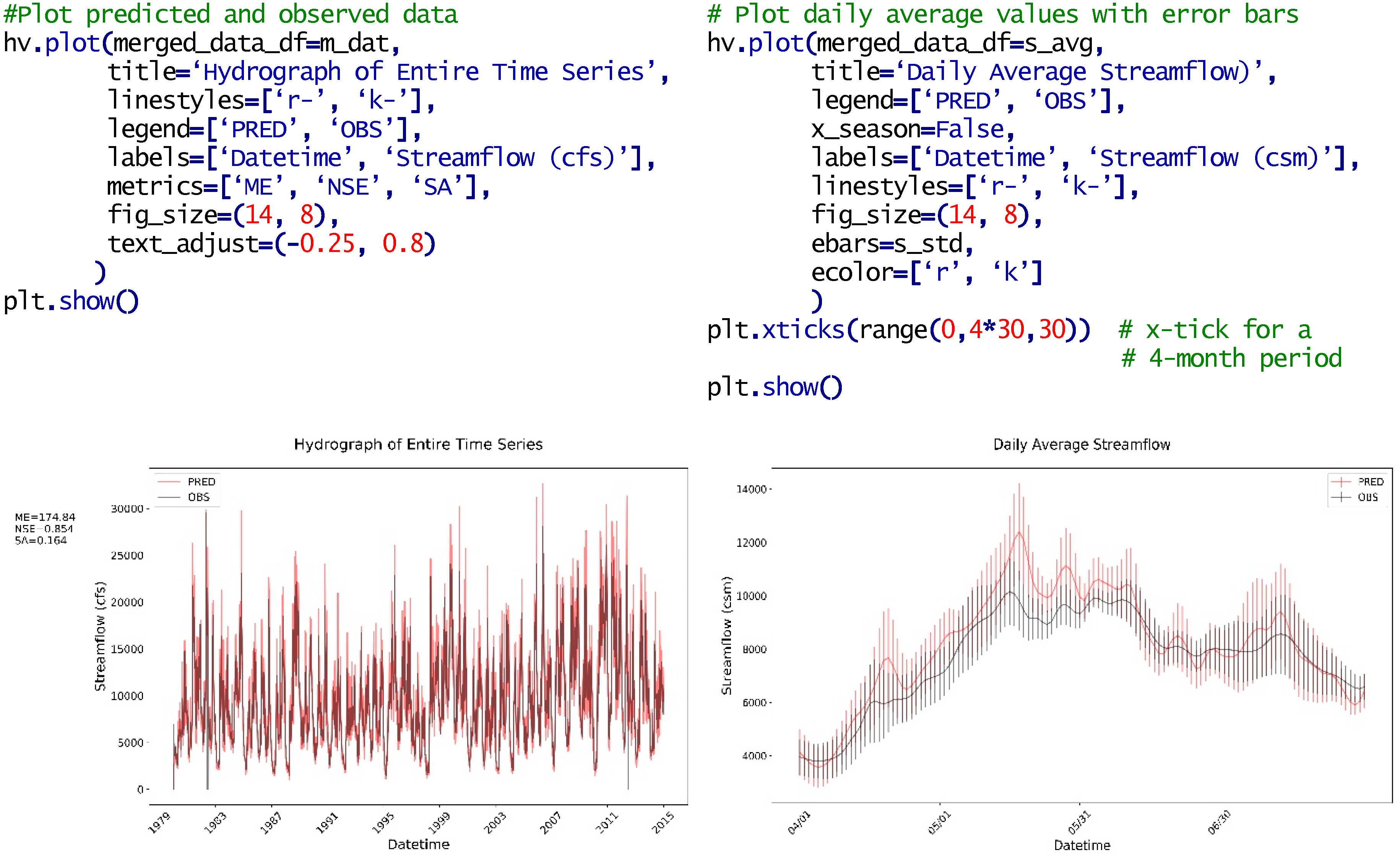
2.5. Visualization (hydrostats.visualization)

Visualization is a powerful tool for understanding model fit and identifying general trends between the modeled and observed flows. Hydrostats includes a few visualization functions based on the Matplotlib package [8]. These functions create custom plots, with the option to display error metrics on the plot, with a user-friendly syntax. The hydrostats.visualization module contains functions to create line plots (called hydrographs in hydrology), plots with error bars, histograms, scatter plots, and q–q (quantile–quantile) plots. Users can generate more advanced plots using the panda data frame object to select data from specific periods then using other Python plotting routines.
Figure 3 shows a code snippet that plots the predicted and observed seasonal values from 1980 to 2015 that were loaded in Figure 2 (left panel), then plots the daily average with error bars for the April to July period (right panel). Visual examination of the left panel, which shows plots of the predicted and observed data, seems to indicate that there is good agreement between the two time series. Visual examination of the right panel is more interesting. This plot presents the daily average with error bars on a daily basis. In this plot, while the fit between the two time series is good, it appears that the fit during May is not as good, this is difficult to see this issue in the left panel. This demonstrates how visualizations and plots can highlight various issues in the data not apparent from line graphs or even with error metrics.

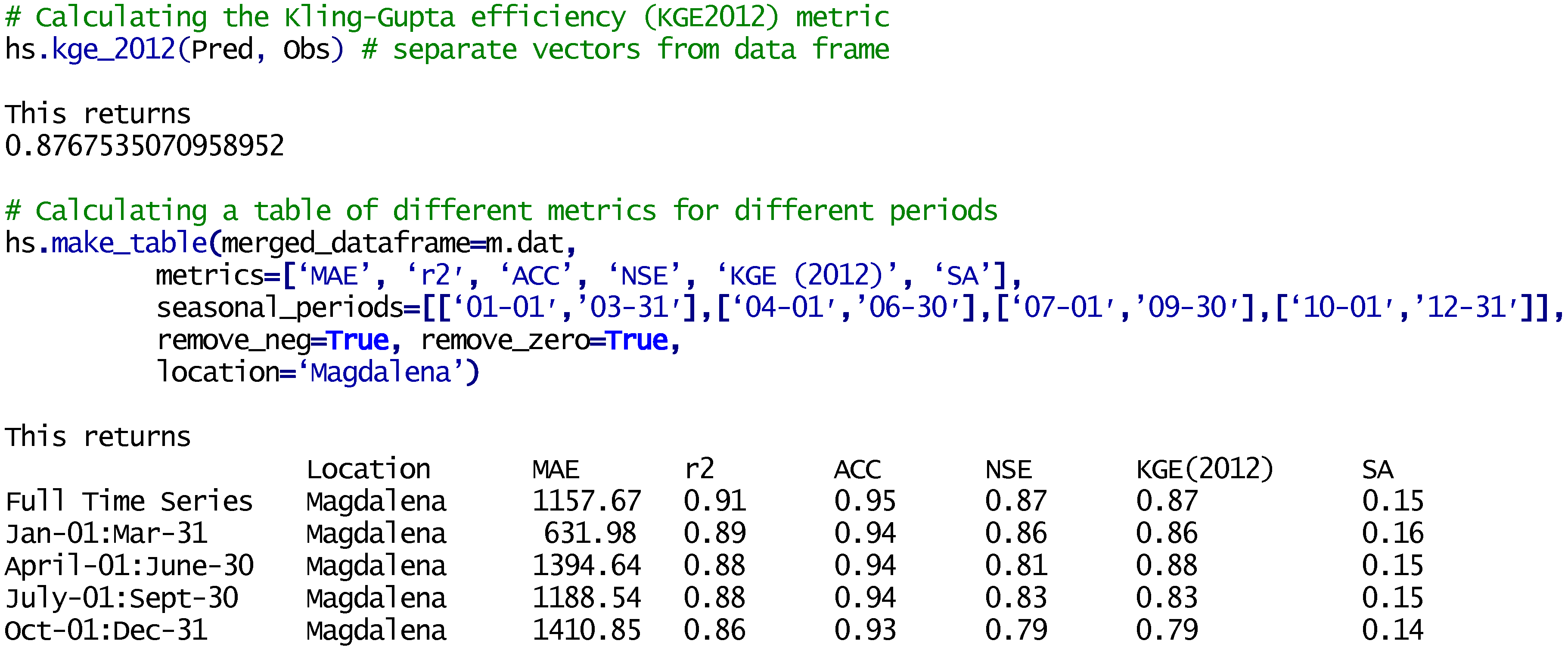
2.6. Error Metrics (hydrostats.metrics)

The hydrostats.metrics module is a wrapper module for the Python HydroErr package, which is available separately. This module gives users access to over 70 error metrics from the hydrologic literature. The HydroErr metric functions can optionally check for 0 (zero) or negative values, and they check for missing values by default. The Python error functions have four flags: replace_nan, replace_inf, remove_neg, and remove_zero. The default behavior (i.e., flags not set) is to remove any data with nan and inf values. HydroErr removes the data from both the predicted and observed vectors and gives a warning to users. For example, if the observed data has missing values, indicated by nan’s, these nan values, along with the corresponding data from the simulated vector, are deleted. This shortens the vectors. Default behavior retains zero or negative values. The replace_neg and replace_inf flags provide values used to replace any instances of these entries, while the remove_neg and remove_zero flags instruct the functions to remove any instances of these values. If an entry is removed in one vector, the corresponding entry is removed from the other vector. If the value is changed to a specified value using the replace_nan or replace_neg flags, the corresponding value in the other vector is unchanged. All of the metrics return the calculated metric value. For all of the parameters that remove data, the function will provide a user with a warning message with a list of all the rows that were removed (i.e., 0, negative, inf, or nan).
Figure 4 presents two function calls using the merged data from Figure 2. The first computes a single error metric, Kling–Gupta efficiency (KGE2012) [20], which returns a single value. The second function call produces a table of six different error metrics, mean absolute error (MAE), coefficient of determination (r2), anomaly correlation coefficient (ACC) [21], KGE2012, and spectral angle (SA) [22], over five different time periods, this table of metrics includes evaluating the full data set, and four different seasons. This demonstrates how easily different error metrics can be used, each of which can highlight different aspects of model accuracy or fit, and different seasons or period evaluated.

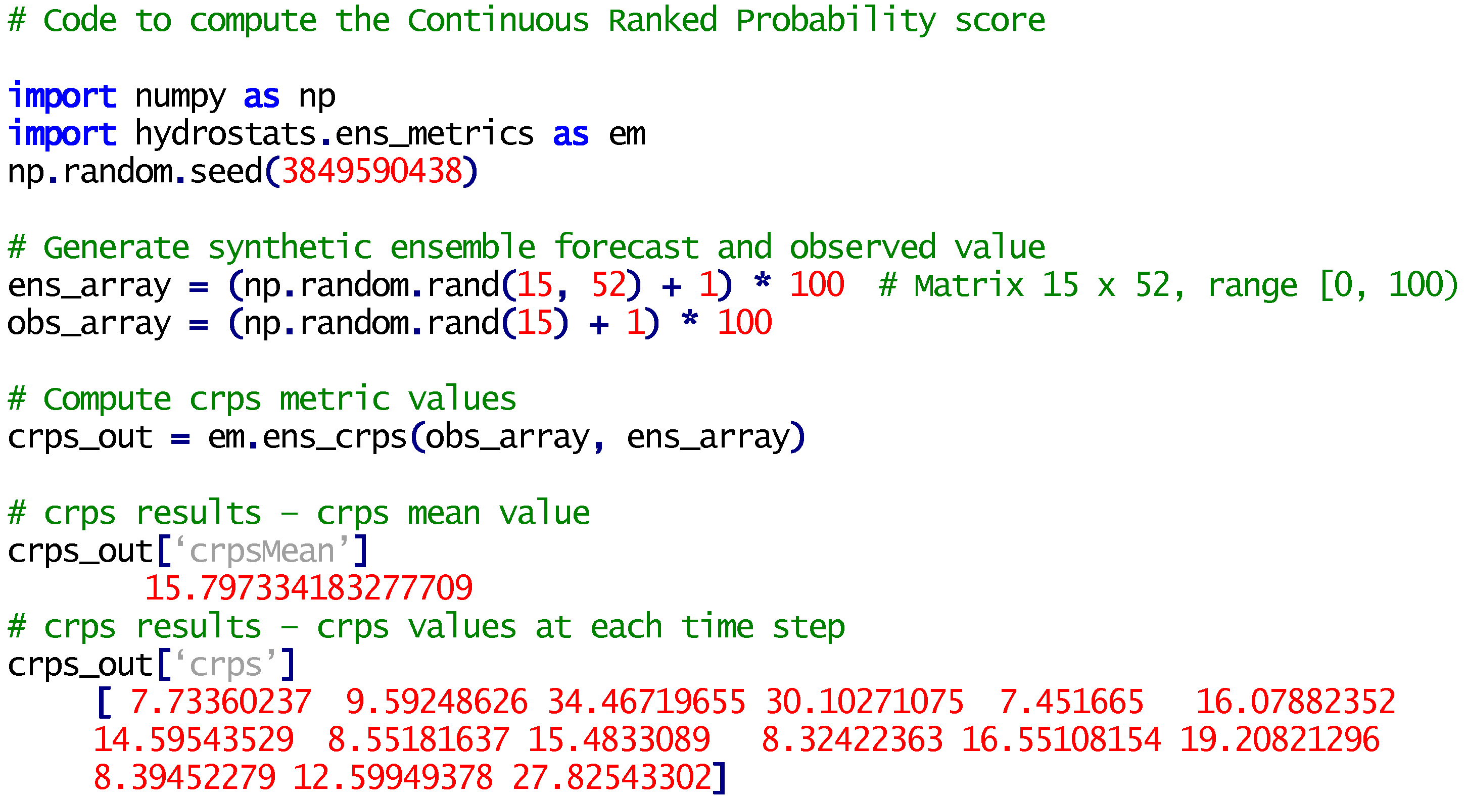
2.7. Forecast Error Metrics

The hydrostats.ens metrics contains many commonly used metrics to gauge forecast skill for stochastic modeling, such as the ensemble mean squared error (EMSE), the continuous ranked probability score (CRPS) [23,24], the area under the receiver operating characteristic curve (AUROC) [25,26], and the ensemble adjusted brier score (EABS) [24]. The hydrostats documentation provides examples and reference for each function in this module.
We give a brief example using the CRPS in Figure 5. The code first loads numpy and the hydrostats.ens_metric package as “em”. Figure 5 lists code that generates a synthetic ensemble forecast of 52 realizations with 15 time steps (ens_array). We arbitrarily selected the forecast length of 15 time steps and the ensemble forecast size of 52 realizations. The code generates an observation of the same length (obs_array) then calls the CRPS metric with the ensemble forecast and observation as inputs.

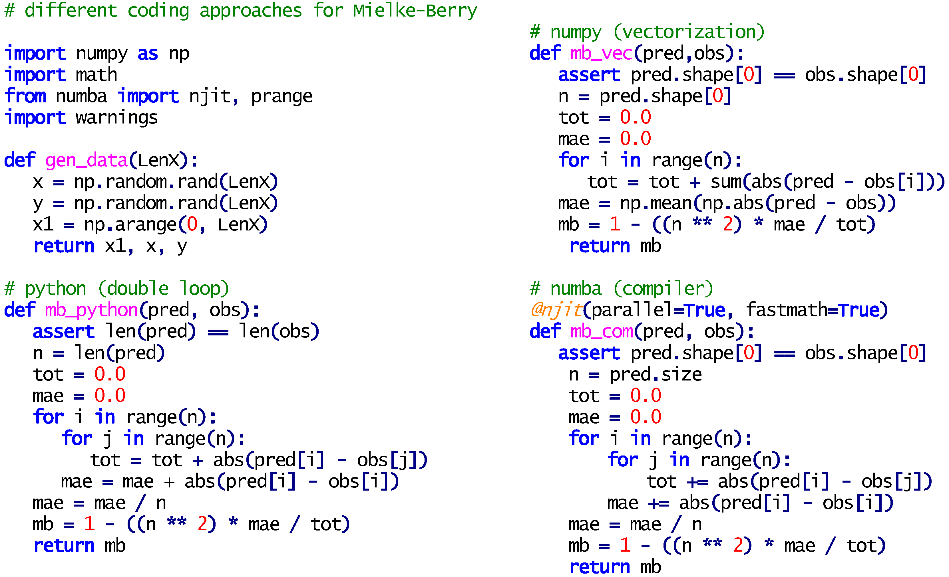
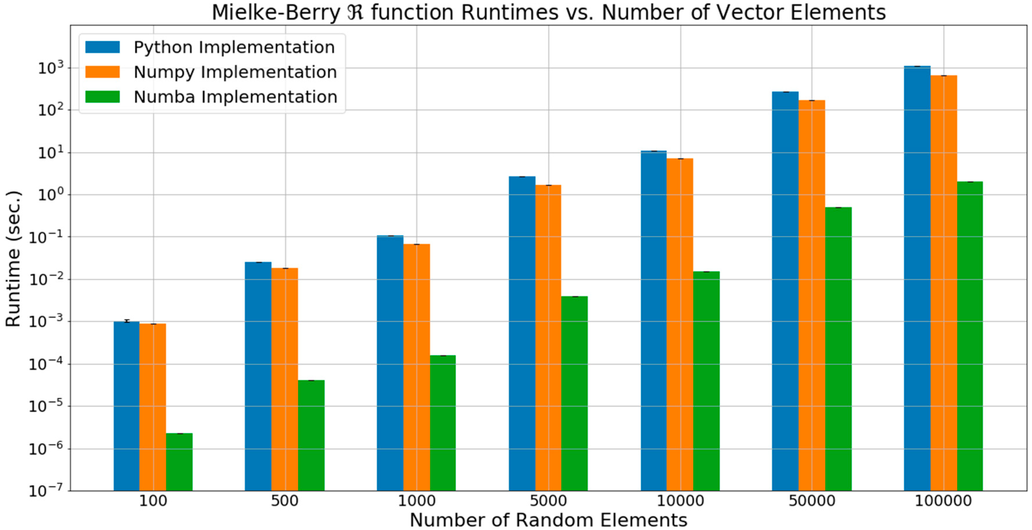
2.8. Code Optimization

We used the Python library NumPy [15,27], an open-source Python package for numerical methods and scientific computations to vectorize functions and provide a more “mathematical” notation in the code. NumPy is significantly faster working with long vectors of data, such as time series records, than using loops in Python, sometimes by one to two orders of magnitude (e.g., 10× to 100× speed-ups) [15]. In the documentation, we provide instructions, where appropriate, to implement Numba [17], which is a just-in-time compiler for Python code using the LLVM compiler infrastructure [17] that can provide similar speed ups over NumPy for certain constructions, such as double loops.
To demonstrate these speed ups we will use the Mielke–Berry R error metric [28] as this error metric requires a double summation as shown in Equation (1).
= 1 M A E n 2 i = 1 n j = 1 n | y i x i |
where MAE (mean absolute error) [29] is:
M A E = 1 n i = 1 n | y i x i |
In Equations (1) and (2), n is the number of data points, x is the observed flow, and y is the predicted flow.
To demonstrate the behavior of different programing approaches, we implemented each using Jupyter Notebook [14] and used the timeit, which times a code function by repeatedly running the function and averaging the runtime. We generated two vectors of random numbers to use as the predicted and observed flows using the numpy.random.rand function which generates numbers in a uniform distribution with values in the range (0 to 1).
Figure 6 presents three different coding approaches that implement the Mielke–Berry error metric. The three coding methods are standard Python, the numpy library, and numba compiler. The Python implementation has a double loop, the numpy method uses vectorization, and the numba approach uses the same loop code as the Python implementation with a command that compiles the code. In Figure 6, the methods are called mb_python, mb_vec, and mb_com, for the double loop, vectorized, and compiled methods, respectively.
To implement the numba compilation, the programmer inserts a Python decoration statement. In Figure 6, the first line of the numba code starts with the decorator statement @njit(parallel=True, fastmath=True). This statement instructs numba to compile this function with options for parallel processing and using fastmath compiler options. The numba compiler does not work with numpy arrays so the code is written in straight Python with a double-loop structure. With the exception of the decorator, the code is the same as that in the mb_py function.
For comparisons, we use the standard python method, mb_python, which is a double loop, as the reference method to compute computational speedup values.
For a vector of length 1000, the numpy version gives a speed up of ~1.5 and the compiled version gives a speedup of ~700. With average function times of 181 × 10−3 ±   9.13 × 10⁻³, 120 × 10−3 ±   8.86 × 10⁻³, and 254 × 10−6 ±   7.03 × 10⁻⁶ s for the python, numpy, and numba implementations, respectively. The speedup is similar with larger vectors. For a vector with 10,000 values the average times go to 16.6, 11.3, and 24.7 × 10⁻³ s for the python, numpy, and numba implementations, respectively, which gives speed ups of ~1.5 and ~675 for the numpy, and numba methods, respectively over the python loops.
Figure 7 shows the results of the three implementations with vector lengths of 100, 500, 1000, 5000, 50,000, and 100,000. For short vectors, while the numba code is significantly faster, all versions run in less than a second. For the longer vectors, the timesavings can be significant. For the 100,000-length vector, the Python version takes over 1000 s (~16 min) while the numba version runs in a few seconds, a significant time difference.
Figure 7 is a semi-log plot that presents these results, in all cases the numba version (i.e., compiled) is over two orders of magnitude (i.e., over 100×) faster than the Python or Numpy versions. As the vector length increases, the numpy version performs faster than the Python version, about 2× to 5× as the vector length increases.
As the results and Figure 7 show, the compiled code is at least two orders of magnitude (200×) faster than the other versions, though for shorter vectors (i.e., less than 1000) the time difference may not be significant.
While the numba compiled code is significantly faster, we did not implement numba versions in the library. This level of speed up only occurs for double loops and only a few of the error metrics require double loops for implementation. Single loops optimize well with numpy implementations. If we had implemented these few metrics requiring double loops using the numba library, then the hydrostats package would have required installing the numba library. We made a decision to not require this dependency, as the vectorized version is sufficiently fast for the majority of the cases. The documentation for the metrics that would benefit from numba compilation have directions on how to modify the code to use numba.

3. Conclusions

This manuscript presents the open-source Python package hydrostats as a resource to evaluate model results for the field of water resource engineering. We hope this package facilitates better practices for model evaluation and calibration. We encourage others to extend and contribute to this effort. The package provides routines to aid with data input, data selection (e.g., specific seasons or times), visualization, and error quantification. We expect one of the major benefits to the using the package is the ability to easily select data from given time periods, such as spring runoff, and generate plots or error metrics. The data frames provide simple methods to perform other analysis, such as evaluating how the error changes as the predicated time series is lagged, to determine if there is a timing offset in the model.
While all the error metrics implemented in the hydrostats package are reported in the literature and most are relatively simple to implement, the hydrostats package will facilitate comparisons of modeled and observed data allowing modelers to easily read data, select and compare specific time periods, use multiple error metrics to quantify model fit, and implement visualizations to evaluate results and identify trends and issues.
Going forward, we hope modelers will use the hydrostats package as a community resource contributing new and revised error metrics or visualizations to make them more widely available to the hydrologic community.
Source code is available at the project home page:
Detailed documentation and references are available at:

Supplementary Materials

The following are available online at https://www.mdpi.com/2306-5338/5/4/66/s1: a Jupyter Notebook with that contains Hydrostats use examples.

Author Contributions

Conceptualization, W.R., E.J., G.P.W. and E.J.N.; methodology, W.R., G.P.W. and D.P.A.; formal analysis, W.R. E.J. and G.P.W.; writing—original draft preparation, W.R. and G.P.W.; writing—review and editing, W.R., G.P.W., D.P.A. and E.J.N.

Funding

This work was supported by the SERVIR, NASA Applied Sciences Program, Grant Number NNX16AN45G.

Conflicts of Interest

The authors declare no conflict of interest. The funders had no role in the design of the study; in the collection, analyses, or interpretation of data; in the writing of the manuscript, or in the decision to publish the results.

References

  1. Snow, A.D.; Christensen, S.D.; Swain, N.R.; Nelson, E.J.; Ames, D.P.; Jones, N.L.; Ding, D.; Noman, N.S.; David, C.H.; Pappenberger, F. A high-resolution national-scale hydrologic forecast system from a global ensemble land surface model. JAWRA J. Am. Water Resour. Assoc. 2016, 52, 950–964. [Google Scholar] [CrossRef]
  2. Swain, N.R.; Christensen, S.D.; Snow, A.D.; Dolder, H.; Espinoza-Dávalos, G.; Goharian, E.; Jones, N.L.; Nelson, E.J.; Ames, D.P.; Burian, S.J. A new open source platform for lowering the barrier for environmental web app development. Environ. Model. Softw. 2016, 85, 11–26. [Google Scholar] [CrossRef] [Green Version]
  3. Reich, N.G.; Lessler, J.; Sakrejda, K.; Lauer, S.A.; Iamsirithaworn, S.; Cummings, D.A. Case study in evaluating time series prediction models using the relative mean absolute error. Am. Stat. 2016, 70, 285–292. [Google Scholar] [CrossRef] [PubMed] [Green Version]
  4. Krause, P.; Boyle, D.; Bäse, F. Comparison of different efficiency criteria for hydrological model assessment. Adv. Geosci. 2005, 5, 89–97. [Google Scholar] [CrossRef]
  5. Roberts, W. Hydrostats-Python Package. Available online: https://pypi.org/project/hydrostats/ (accessed on 30 September 2018).
  6. Roberts, W. Hydrostats Source Code—Github. Available online: https://github.com/BYU-Hydroinformatics/hydrostats/ (accessed on 30 September 2018).
  7. McKinney, W. Python for Data Analysis: Data Wrangling with Pandas, Numpy, and Ipython; O’Reilly Media, Inc.: Boston, MA, USA, 2012. [Google Scholar]
  8. Hunter, J.D. Matplotlib: A 2d graphics environment. Comput. Sci. Eng. 2007, 9, 90–95. [Google Scholar] [CrossRef]
  9. Roberts, W. Hydroerr—Hydrologic Error Metrics, Python Library. Available online: https://pypi.org/project/HydroErr/ (accessed on 30 September 2018).
  10. Roberts, W. HydroErr Documentation—Github. Available online: https://byu-hydroinformatics.github.io/HydroErr/ (accessed on 30 September 2018).
  11. Roberts, W. HydroErr Source Code—Github. Available online: https://github.com/BYU-Hydroinformatics/HydroErr (accessed on 30 September 2018).
  12. Roberts, W. Hydrostats Documentation—Github. Available online: https://byu-hydroinformatics.github.io/Hydrostats/ (accessed on 30 September 2018).
  13. Roberts, W. A python package for computing error metrics for observed and predicted time series. In 9th International Congress on Environmental Modeling & Software; International Environmental Modeling & Software Society: Fort Collins, CO, USA, 2018. [Google Scholar]
  14. Kluyver, T.; Ragan-Kelley, B.; Pérez, F.; Granger, B.E.; Bussonnier, M.; Frederic, J.; Kelley, K.; Hamrick, J.B.; Grout, J.; Corlay, S. Jupyter Notebooks—A publishing Format for Reproducible Computational Workflows; ELPUB: Amsterdam, Netherlands, 2016; pp. 87–90. [Google Scholar]
  15. Oliphant, T.E. A Guide to Numpy; Trelgol Publishing: Provo, UT, USA, 2006; Volume 1. [Google Scholar]
  16. Jones, E.; Oliphant, T.; Peterson, P. SciPy: Open Source Scientific Tools for Python. Available online: http://www.scipy.org/ (accessed on 30 September 2018).
  17. Lam, S.K.; Pitrou, A.; Seibert, S. Numba: A llvm-based python jit compiler. In Proceedings of the Second Workshop on the LLVM Compiler Infrastructure in HPC, Austin, TX, USA, 15–20 November 2015; ACM: Austin, TX, USA, 2015; p. 7. [Google Scholar]
  18. Gazoni, E.; Clark, C. Openpyxl—A Python Library to Read/Write Excel 2010 xlsx/xlsm Files. Available online: https://openpyxl.readthedocs.io/en/stable/ (accessed on 30 September 2018).
  19. McKinney, W. Data structures for statistical computing in python. In Proceedings of the 9th Python in Science Conference, Austin, TX, USA, 28–30 June 2010; pp. 51–56. [Google Scholar]
  20. Kling, H.; Fuchs, M.; Paulin, M. Runoff conditions in the upper danube basin under an ensemble of climate change scenarios. J. Hydrol. 2012, 424, 264–277. [Google Scholar] [CrossRef]
  21. Murphy, A.H.; Epstein, E.S. Skill scores and correlation coefficients in model verification. Mon. Weather Rev. 1989, 117, 572–582. [Google Scholar] [CrossRef]
  22. Robila, S.A.; Gershman, A. Spectral matching accuracy in processing hyperspectral data. In Proceedings of the International Symposium on Signals, Circuits and Systems, 2005, ISSCS 2005, Iasi, Romania, 14–15 July 2005; pp. 163–166. [Google Scholar]
  23. Gneiting, T.; Raftery, A.E. Strictly proper scoring rules, prediction, and estimation. J. Am. Stat. Assoc. 2007, 102, 359–378. [Google Scholar] [CrossRef]
  24. Ferro, C.A.; Richardson, D.S.; Weigel, A.P. On the effect of ensemble size on the discrete and continuous ranked probability scores. Meteorol. Appl. 2008, 15, 19–24. [Google Scholar] [CrossRef] [Green Version]
  25. DeLong, E.R.; DeLong, D.M.; Clarke-Pearson, D.L. Comparing the areas under two or more correlated receiver operating characteristic curves: A nonparametric approach. Biometrics 1988, 837–845. [Google Scholar] [CrossRef]
  26. Sun, X.; Xu, W. Fast implementation of delong’s algorithm for comparing the areas under correlated receiver operating characteristic curves. IEEE Signal Process. Lett. 2014, 21, 1389–1393. [Google Scholar] [CrossRef]
  27. Walt, S.v.d.; Colbert, S.C.; Varoquaux, G. The numpy array: A structure for efficient numerical computation. Comput. Sci. Eng. 2011, 13, 22–30. [Google Scholar] [CrossRef]
  28. Mielke, P.W.; Berry, K.J. Permutation Methods: A Distance Function Approach; Springer Science & Business Media: New York, NY, USA, 2007. [Google Scholar]
  29. Willmott, C.J.; Matsuura, K. Advantages of the mean absolute error (mae) over the root mean square error (rmse) in assessing average model performance. Clim. Res. 2005, 30, 79–82. [Google Scholar] [CrossRef]
Figure 1. Example code showing loading of the hydrostats package, modules, and other dependencies.
Hydrology 05 00066 g001
Figure 2. Presents an example of code and results. The code loads two .csv files into a single data object with named columns (line 1), then extracts the data from 1 April to 31 July from the period 1 January 1986 through 31 December 1994. Below the code are the first and last three lines of the merged data frame, m_dat, and the daily average, s_avg, data frame. We do not show the data from the standard deviation data frame, s_std.
Hydrology 05 00066 g002
Figure 3. Presents an example of hydrostat.visual code and plots that show the simulated and observed data (left panel) and daily averages over a season from April to July (right panel). The plots use the data from Figure 2, the m_dat data frame for the entire record, and the s_avg and s_std data frames for the daily averages with error bars over a shorter season. Note that in the right panel, in addition to the plot, the results from three different error metrics are included.
Hydrology 05 00066 g003
Figure 4. Presents a code example and results of calling a single error metric (top portion) and creating a table with six different error metrics over four different seasons or time periods. This shows that while the metric values are similar, the different seasons behave differently.
Hydrology 05 00066 g004
Figure 5. Presents a code example and results for computing the Continuous Ranked Probability Score (CRPS) for an ensemble forecast with 52 realizations and a length of 15. The bottom of the figure shows the CRPS mean, and the CRPS values at each time step.
Hydrology 05 00066 g005
Figure 6. Three different coding approaches to implementing the Mielke–Berry error metric which requires a double summation. The three coding methods are python, numpy, and numba, which implements a double loop, vectorization, and compiled code, respectively. The @njit line in the numba implementation is the instruction that instructs the compiler to compile this function. For a vector of length 1000, the numpy version gives a speed up of ~1.5 and the compiled version gives a speedup of ~700. With average function times of 181 × 10−3 ±   9.13 × 10⁻³, 120 × 10−3 ±   8.86 × 10⁻³, and 254 × 10−6 ±   7.03 × 10⁻⁶ s for the python, numpy, and numba implementations, respectively.
Hydrology 05 00066 g006
Figure 7. Runtimes for three different implementations of the Mielke–Berry R metric, plotted with a logarithmic vertical axis. Benchmarks were performed using 7.7 GB of RAM and an Intel® CoreTM i5-4590 CPU @ 3.30 Ghz x 4.
Hydrology 05 00066 g007

