Calibration and Validation of an Operational Method to Estimate Actual Evapotranspiration in Mediterranean Wetlands

Abstract

A semi-empirical method for estimating actual evapotranspiration (ETa) based on ancillary and NDVI data, named NDVI-Cws, is currently being refined for improved applicability to wetlands. The investigation, in particular, addresses the case of semi-natural ecosystems where the impact of meteorological water stress (WS) is limited by groundwater resources. To adapt to this situation, the application of the NDVI-Cws method is preceded by a calibration phase based on spatially enhanced Land Surface Analysis Satellite Application Facility (LSA SAF) evapotranspiration products. This calibration is currently performed in the main wetlands of Tuscany (Central Italy) identified in the Ramsar Convention. The calibrated NDVI-Cws version is then applied to all regional Ramsar areas, yielding outputs that are first examined all over Tuscany. Next, the model estimates are quantitatively assessed versus ETa observations taken in a forest and a grassland Ramsar site. The results of these independent tests show the improvement achieved by the calibration phase with respect to the original model version. This supports the potential of the refined NDVI-Cws method to yield reasonably accurate daily ETa estimates for wetlands at a spatial resolution that is mainly dependent on the NDVI data used.

1. Introduction

Actual evapotranspiration (ETa), defined as the sum of evaporation (from soil and plant surface) and transpiration (from vegetation), is a fundamental component of the land–water cycle. ETa is controlled by both physical and biological factors that show high spatio-temporal variability and are expected to be influenced by the increased drought frequency and intensity caused by global warming [1,2]. This promotes the utility of monitoring ETa, which is particularly felt in water-limited regions such as those surrounding the Mediterranean basin [3,4].

Remote sensing techniques have been widely applied for ETa prediction due to their capacity to monitor land surface features with high spatial and temporal resolutions [5,6]. These techniques are usually categorized into energy balance, water balance, and mixed methods [7]. Energy balance ETa estimation methods offer the advantage of directly assessing the water fluxes coming from the examined land surface and have, therefore, been widely investigated and applied [8]. These methods, however, are affected by two main issues. First, the actual temporal frequency of good-quality thermal infrared (TI) imagery may be significantly reduced by atmospheric disturbances, which are obviously more frequent in humid areas and periods [9]. Second, the spatial resolution of the available TI imagery is generally low, and this issue can be only attenuated by the application of spatial sharpening procedures which introduces additional uncertainty [10].

Water-balance methods, which rely on the Food and Agriculture Organization (FAO) crop coefficient (Kc) concept [11], are less affected by the aforementioned spatio-temporal resolution issues. These methods, in fact, usually derive the Kc of the examined vegetation from optical satellite data through the use of vegetation indices (VIs), that are quite stable and can be easily interpolated in time. On the other hand, water-balance methods are intrinsically affected by another drawback, i.e., the poor capability of characterizing ETa decreases due to short-term water stress (WS). This is due to the limited information contained in optical imagery about stomata closure and other rapid (and reversible) plant adaptation mechanisms induced by transient dry spells [12].

The first versions of the water-balance models were, therefore, conceived for monitoring the ETa of vegetated areas not significantly affected by WS [13]. These methods were then extended to deal with water-limited ecosystems relying on ancillary information, which includes conventional or remotely sensed meteorological observations. The Veg-ET model developed by [14,15], for example, incorporates a scalar similar to the FAO WS coefficient (Ks) derived from a site water balance, which requires the use of soil information in addition to meteorological data. The common scarcity of accurate information on soil properties is circumvented in the NDVI-Cws method proposed by [16], through the combination of conventional meteorological data and satellite normalized difference vegetation index (NDVI) images. Transient WS is assumed to induce rapid and reversible transpiration reduction, while more intense, long-term water shortage causes substantial and irreversible green biomass loss. Two meteorological short-term WS scalars, one for transpiration and the other for evaporation, are, therefore, used to reduce transpiration to half of its potential and evaporation to zero; long-term effects of WS are assumed to be accounted for by an NDVI reduction [16].

Several tests performed in different Mediterranean environments have supported the general efficiency of the NDVI-Cws method while also highlighting a limitation that can degrade its performance in specific cases. All methods that simulate WS’s impact on vegetation relying on meteorological observations, in fact, are sensitive to the possible supply of water from sources additional to rainfall, which commonly correspond to irrigation for croplands and to a shallow water table for semi-natural ecosystems. The former case was addressed by [17], who proposed a modification of the NDVI-Cws method aimed at predicting the ETa and irrigation water (IW) in areas grown with summer crops. Fibbi et al. [18] have instead put forward a calibration procedure that addresses the case of semi-natural ecosystems based on Land Surface Analysis Satellite Application Facility (LSA SAF) ET products and Moderate-Resolution Imaging Spectroradiometer (MODIS) TI imagery. In both cases, the WS scalars of the NDVI-Cws model are modified to consider the water additional to rainfall provided to local plants during part of the growing season or constantly.

The calibration approach proposed by [18] is potentially usable for extending the application of the NDVI-Cws method to wetlands, which are globally identified and characterized by the Ramsar Convention [19]. This operation is currently carried out concerning Tuscany, a region in Central Italy characterized by high spatio-temporal variability in land surface features and conditions. In particular, the current research is aimed at refining and testing the NDVI-Cws method for application to all Ramsar areas of the region; building on the aforementioned studies, these operations are based on the use of integrated LSA SAF ET and MODIS TI datasets.

The paper is organized into the following main sections: the first introduces the materials and methods utilized to apply the NDVI-Cws model and modulate its WS coefficients, followed by the testing of the modified method in two case studies. The next section reports the results achieved during these activities, which are discussed and commented on in the final section.

2. Materials and Methods

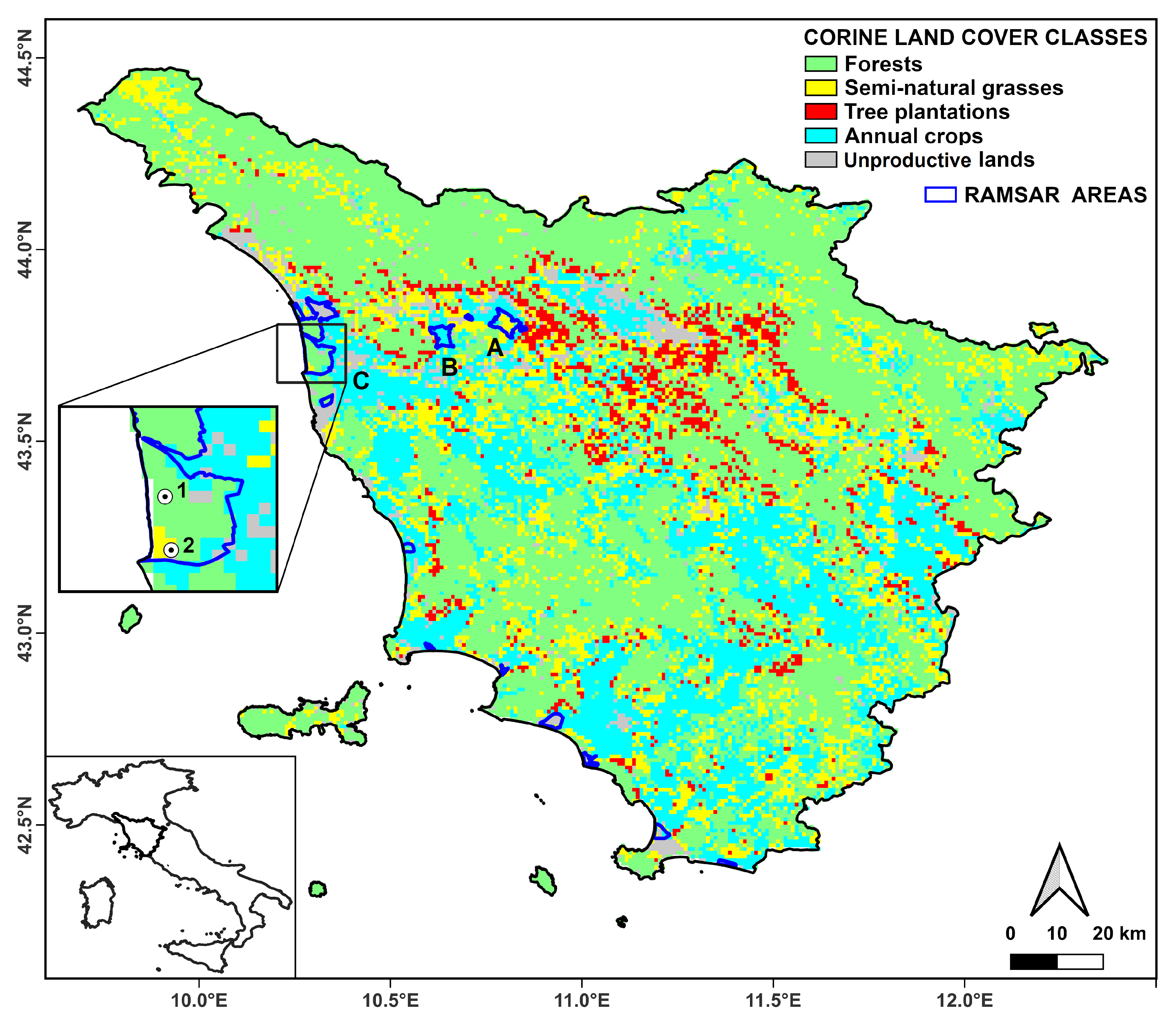
2.1. Study Region

Tuscany is a region of Central Italy characterized by the presence of plain and hilly areas, and the Apuan Alps and Apennines Mountain chains (Figure 1). Its altitude ranges from the sea level to about 2000 m a.s.l. and its climate varies from Mediterranean warm (mean annual temperature, Tmean, about 16.5 °C) to temperate cool (Tmean about 10.5 °C), following the latitudinal and altitudinal gradients and the distance from the sea. About half of Tuscany is covered by forests (about 1,090,000 ha), which are mostly located on higher hills and mountains. Extensive wetlands are present in the north and near the coastline of the region; their geographic position, derived from the Ramsar database (see https://rsis.ramsar.org/) (accessed on 10 January 2025), is shown in Figure 1.

The same figure shows the location of the three widest Ramsar wetlands of the region covered by semi-natural vegetation (forest and grassland), which were used for calibrating the NDVI-Cws method: Fucecchio (A), Migliarino (B) and San Rossore (C). The former site is mostly covered by grasslands and some hygrophilous tree species (mostly Populus spp.). The latter two sites are coastal lowlands covered by artificial Mediterranean pine forests (mostly Pinus pinea L.) planted about 100 years ago. These areas, the main environmental characteristics of which are summarized in

Table 1. Main characteristics of the selected Ramsar areas shown in Figure 1; the meteorological data are averaged over the five study years (2019–2023).

Ramsar Area	Geographical Position	Altitude (m a.s.l.)	Area (km2)	Mean Annual Temperature (°C)	Annual Rainfall (mm)	Main Biome Type
A	43.80° N, 10.80° E	20	24.4	15.9	960	Grassland
B	43.79° N, 10.30° E	5	38.1	16.2	921	Forest
C	43.72° N, 10.31° E	5	69.2	16.3	924	Forest

, were selected to minimize the effects of agricultural activities in cropped lands, as well as the influence of mixed and boundary pixels.

The testing of the calibrated NDVI-Cws method was performed in two sites corresponding to a pine forest and a grassland, both included within the San Rossore area (Pisa, Italy; 43.68–43.78° Lat. N, 10.27–10.34° Long. E) (Figure 1). The soil of both sites is mostly sandy, with the deepest layers which are rarely fully dried due to the presence of a shallow soil water table which reduces the sensitivity of local vegetation to WS.

2.2. Study Data

2.2.1. Eddy Covariance Observations

A micrometeorological station was installed in 2012 within an even-aged Pinus pinea L., 1753 (Stone pine or umbrella pine) stand of the San Rossore forest (Figure 1) and became the official San Rossore 2 ICOS (Integrated Carbon Observation System) Class 2 Ecosystem Station in December 2019 (https://meta.icos-cp.eu/resources/stations/ES_IT-SR2) (accessed on 10 January 2025). All measurements, including turbulent fluxes of latent and sensible heat, are centrally quality checked and processed according to the ICOS standards [20] by the ICOS-ETC (Ecosystem Thematic Centre), and to the overall FLUXNET2015 procedures [21].

The even-aged forest normally covers an area of 37.62 ha (also defined as ICOS Target Area) and presents a high degree of homogeneity in terms of vegetation cover and structure. The flux footprint is almost always comprised within this surface, making the flux measurements reliably representative of the target area [22,23]. The umbrella pine, in fact, is dominant in more than 90% of this area and has uniform and narrow age and height distribution (80–100 years and 19 m, respectively) [23]. The understory is normally not homogeneous, and it is composed of Mediterranean maquis species of variable height between a few cm and 5 m (mostly Erica arborea L., 1753 and Myrtus communis L., 1753).

Latent heat flux measurements, corresponding to the surface evapotranspiration, were collected over the five-year study period (2019–2023) at half-hourly resolution and, after conversion into mm and integration over a daily resolution, were assumed as estimates of the daily ETa. Micrometeorological data were downloaded from the ICOS Carbon portal (https://hdl.handle.net/11676/QFiihIGr2XHkETyfMuOnvb1Z) (accessed on 10 January 2025).

2.2.2. Meteorological Data

Meteorological variables (e.g., air temperature, rainfall, and solar radiation) were collected at the San Rossore 2 eddy covariance site over the years 2019–2023 with a half-hourly resolution, averaged and cumulated to the daily scale. In addition to these, interpolated daily minimum and maximum air temperatures, and rainfall were obtained by applying the DAYMET algorithm to the ground observations of the LaMMA Consortium [24]. Daily solar radiation estimates for the same years were then obtained through the Estimation of global solar RADiation (ERAD) algorithm, which is based on Meteosat Second Generation (MSG) satellite data [25]. All these datasets have a 250 m spatial resolution.

2.2.3. MODIS Images

All Terra MODIS products currently used were downloaded from the United States Geological Survey site (https://e4ftl01.cr.usgs.gov) (accessed on 17 February 2025). The NDVI product (MOD13Q1 v061) was taken as a maximum value composite (MVC) every 16 days, at 250-m spatial resolution [26]. More specifically, 23 NDVI MVC images per year, covering the study area and period (i.e., 2019–2023), were downloaded from the corresponding MODIS tile, further processed to remove residual atmospheric disturbances, and linearly interpolated on a daily basis as described in [16].

The Land Surface Temperature (LST) product (MOD21A1D v061) corresponds to 1-km estimates derived from MODIS thermal infrared bands using the Advanced Spaceborne Thermal Emission and Reflection Radiometer (ASTER) Temperature Emissivity Separation (TES) algorithm [27]. All daily LST cloud-free images over the San Rossore area were downloaded for two selected months (June and August) of the five years 2019–2023.

2.2.4. LSA-SAF Images

Some ET products developed from the EUMETSAT LSA SAF were obtained through the Portuguese Institute for the Sea and Atmosphere (IPMA) (https://datalsasaf.lsasvcs.ipma.pt/PRODUCTS) (accessed on 17 February 2025). These products are produced through physically based and simplified Soil-Vegetation-Atmosphere-Transfer algorithms using data taken by the Spinning Enhanced Visible and Infrared Imager (SEVIRI) sensor, installed onboard the MST geostationary satellite [28]. Currently, two different 5-km daily products were downloaded for the years 2019–2023: (i) the reference evapotranspiration product (METREF LSA-303), and (ii) the last version of the actual evapotranspiration product (DMETv3 LSA-312.3) [29]. From these products, the daily evapotranspiration fraction (i.e., actual over potential evapotranspiration, ETf) was computed for the same period.

2.3. ETa Modelling Strategy

The NDVI-Cws ETa estimation method operates through the combination of satellite NDVI images and conventional meteorological data (i.e., daily air temperature, precipitation, and solar radiation) [16]. The method assumes that transient WS induces rapid and reversible evapotranspiration reduction, while more intense, long-term water shortage causes substantial and persistent green biomass loss. The first factor is accounted for by two short-term WS scalars derived from standard meteorological data, which are used to downregulate both plant transpiration and soil evaporation. The long-term effect of WS is instead assumed to be considered by NDVI reduction [16].

Following this formulation, the fractional vegetation cover (FVC) is used to weigh the contribution of site transpiration and evaporation by means of the following Equation:

ETa = ET0·(KcVeg·FVC·Cws + KcSoil·(1 − FVC)·AW)

(1)

where Cws and AW are the WS scalars for transpiration and evaporation, respectively, KcVeg and KcSoil correspond to the maximum crop coefficients of the examined vegetation type (0.7 for forest and 1.2 for grasses) and soil (0.2), and ET0 corresponds to the reference ET computed following [30].

FVC is usually obtained from NDVI through the generalized linear equation proposed by [31], whilst the two WS scalars are computed as:

AW = Rain/ET0

(2)

Cws = C1 + C2·AW

(3)

where Rain (i.e., rainfall) and ET0 are cumulated over one or two months for grasses and trees, respectively, and their ratio is bound to 1; both coefficients, C1 and C2, are set to 0.5 in the original model configuration [12,16].

This configuration therefore limits the possible downregulation of simulated transpiration to half of its potential maximum, as fully explained in [16]. The actual meteorological WS impact on ETa, however, can be reduced by the provision of water supplemental to rainfall, i.e., irrigation for croplands or shallow groundwater reserves for semi-natural ecosystems. Concerning croplands, Maselli et al. [17] addressed the problem by proposing a modification of the NDVI-Cws method for identifying and quantifying crop irrigation. The prediction of ETa for semi-natural ecosystems where water is supplied by shallow groundwater sources was instead investigated by [32]. These authors proposed a site-specific calibration of the two coefficients of Equation (3) based on the ETf derived from global LSA SAF ET products. More specifically, the calibration is performed by considering the ETf decrease which occurs from the start to the peak of the Mediterranean dry season (i.e., normally from June to August) as an indicator of WS impact on ETa.

As explicitly recognized by the same authors, however, the use of the LSA SAF products introduces a significant spatial resolution issue in heterogeneous landscapes. This issue can be addressed by applying a further correction step based on MODIS LST images, which have a 1-km spatial resolution [18]. The integration of LSA SAF and MODIS data relies on the psychrometric constant theory exposed by [33], which postulates an equivalence between ETf and normalized LST differences. This integration can yield mean 1-km resolution ETf maps of the study periods, which are finally usable to calibrate the NDVI-Cws sensitivity to WS.

2.4. Data Processing

The current calibration of the NDVI-Cws method for ETa estimation of all Tuscany wetlands was based on the mean spatially enhanced LSA SAF ETf images of June and August 2019–2023 produced as described in [18]. In particular, the mean ETf values of August were divided by those of June, and the obtained ratio was taken as an indicator of WS impact on vegetation [32]. This ratio was used to calibrate the C1 and C2 coefficients of the NDVI-Cws method for the three selected Ramsar areas (i.e., Fucecchio, Migliarino, and San Rossore). For each of these areas, the method was fed with interpolated and remotely sensed data of the years 2019–2023, and a sensitivity analysis was performed by varying the C1 and C2 coefficients of Equation (3) from 0.5 to 1.0 and 0.5 to 0.0, respectively, and evaluating the corresponding effect on the simulated ETf ratio. In each case, the same coefficients were then modified to reproduce the reference ETf decrease from June to August obtained from the enhanced LSA SAF ETf product (see [18], for details). The average C1 and C2 values found in this calibration phase were finally applied to all Ramsar areas of Tuscany.

During the testing phase, the ETf decrease from June to August obtained from the LSA SAF products and the NDVI-Cws method were first inter-compared all over the region. The accuracy of the original and calibrated NDVI-Cws versions for wetlands was then evaluated versus the flux tower ETa observations of the San Rossore pine forest. To this aim, the two model versions were fed with meteorological and satellite data extracted from the four 250-m pixels closest to the tower site. The daily ETa estimates of the five study years were compared to the tower ETa observations summarizing the results by means of the Nash-Sutcliffe coefficient of model efficiency (ME), which is commonly used for evaluating hydrological models [34]. ME corresponds to 1 in case of perfect reproduction of the observations, while ME = 0 indicates a reproduction equivalent to the observed average, and negative ME indicates a reproduction worse than the average.

The calibrated NDVI-Cws method was also tested in an area of San Rossore covered by grassland (Figure 1), where reference ETa observations were obtained by a simplified water-balance model already applied in [18]. This model uses a bucket approach to simulate the soil water dynamics and predicts ETa based on the FAO Kc concept [35]. The model was driven by the available ICOS environmental and meteorological observations considering a 0.5 m rooting depth and a 0.25 m water table and provided reference daily ETa data series for the five study years. Also in this case, the Nash-Sutcliffe ME was used to evaluate the accuracy of the daily ETa estimates versus the reference data.

3. Results

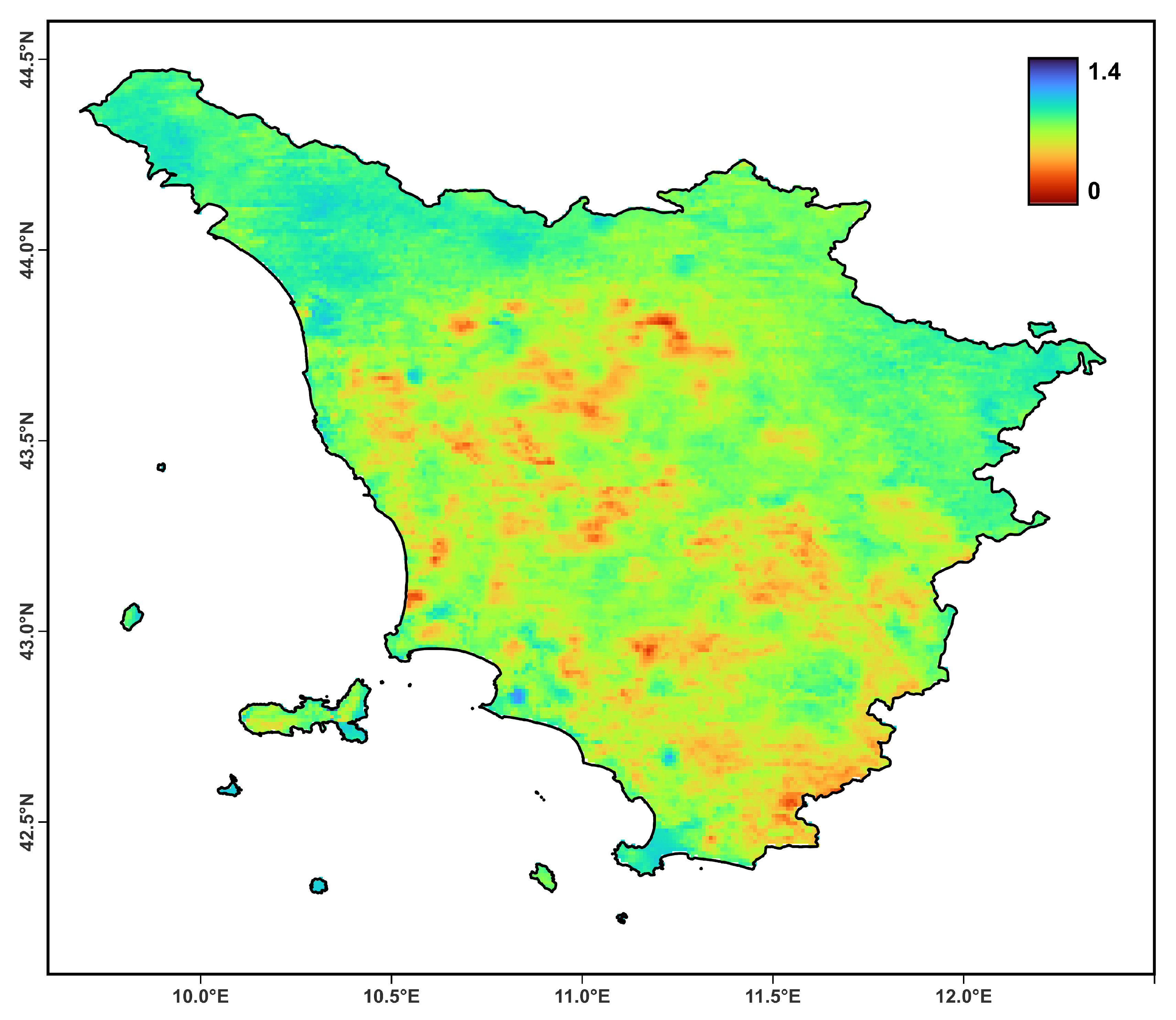
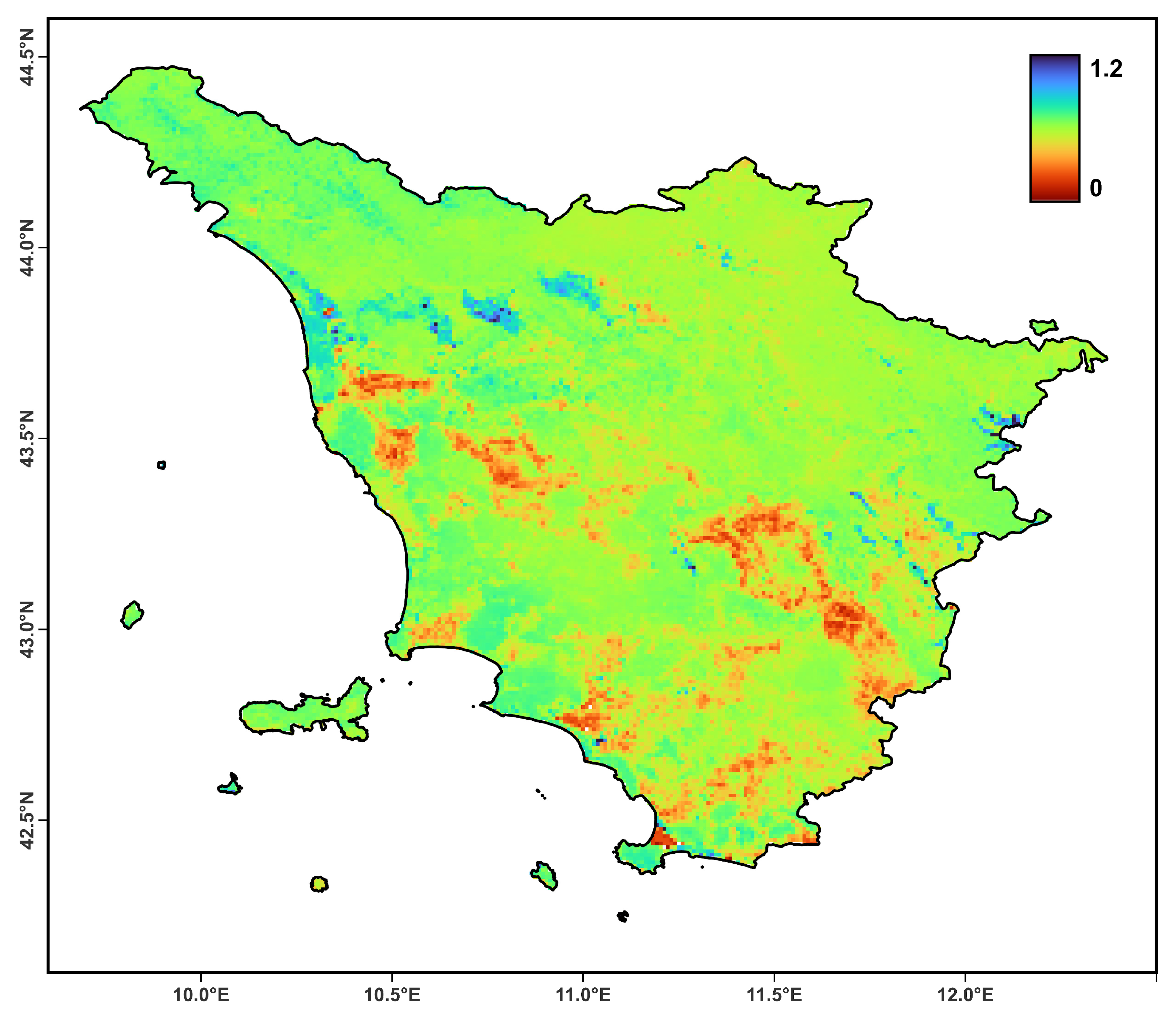
3.1. Regional NDVI-Cws Estimates

Figure 2 shows the ratio between the mean ETf of August and June obtained from LSA SAF and MODIS images. This ratio is inversely proportional to the impact of WS over Tuscany areas, which varies due to both land cover and climate. In general, Ramsar and mountain areas have the highest ratios, while plain croplands have the lowest ratios (i.e., the lowest/highest WS impact, respectively). This is more clearly visible from the average ratios of the five CORINE land cover (CLC) categories and Ramsar areas which are shown in Figure 3.

Figure 4 shows the results of the sensitivity analysis performed over the three selected Ramsar areas, together with the respective optimum C1 values identified by the calibration. For all three sites, the ratio between simulated August and June ETf values increases with the C1 coefficient within Equation (3), indicating a progressively reduced effect of meteorological WS. As expected, all ratios derived from the enhanced LSA SAF images (crosses) are higher than those obtained by the standard NDVI-Cws method (i.e., for C1 = 0.5). The reproduction of these reference ratios, therefore, requires the increase of C1; the optimal C1 values identified in the three cases are quite variable, ranging from 0.64 for Fucecchio (Ramsar A) and 0.67 for San Rossore (Ramsar C) to 0.89 for Migliarino (Ramsar B). These differences can be reasonably attributed to the different environmental features of the three areas, and particularly to the respective groundwater resources which feed local vegetation. Finally, a C1 very close to the arithmetic average (0.75) is identified as optimal for all Ramsar areas of the region, while C2 is obviously set to its complementary value (0.25); these coefficients imply a model sensitivity to WS reduced to half of its original value.

The mean ETf08/ETf06 ratio obtained by applying the complete version of the NDVI-Cws model all over Tuscany for the five study years is displayed in Figure 5. A certain similarity with Figure 2 can be observed, particularly for the highest ETf ratio of the northern mountains and wetlands and the lowest ratio in the southern plains, which are mostly covered by temperate forests and annual crops, respectively. In general, the ratios obtained from NDVI-Cws are slightly lower than those from LSA SAF + LST, which implies a greater WS impact estimated by the former model for most areas of the region.

These observations are confirmed by the mean ratios of the five CLC categories and Ramsar areas shown in Figure 3. The NDVI-Cws ratios are all lower than their LSA SAF counterparts (around 14%) but the agreement between them is high and highly significant (r = 0.920, p < 0.01). This pattern is confirmed for the Ramsar areas, which is apparently in contrast with the results of the calibration phase that is expected to produce similar ETf ratios from the two sources. This finding can be attributed to the consideration of Ramsar areas in addition to those used in the training phase which, being mostly small, are strongly contaminated by mixed and boundary pixels (Figure 1).

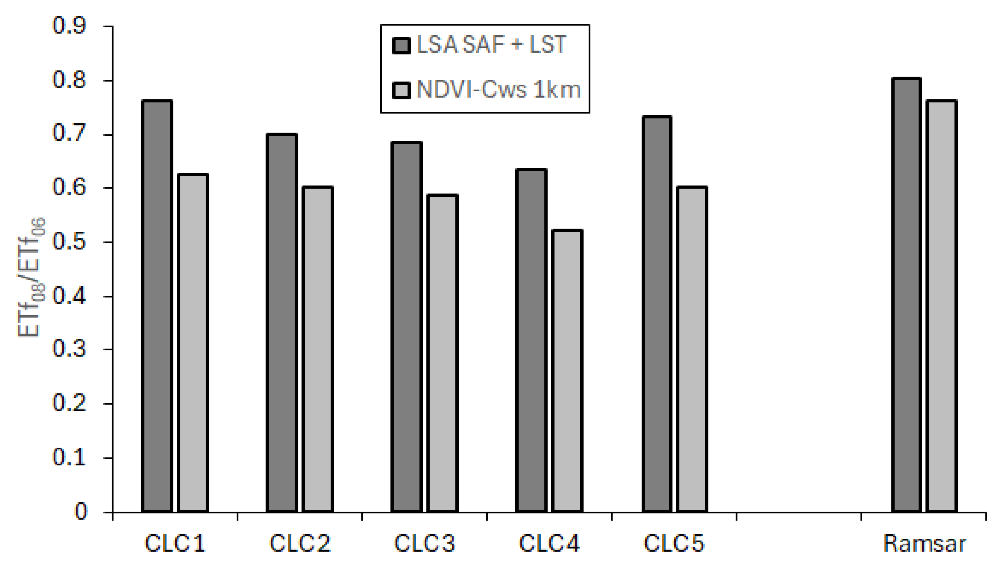
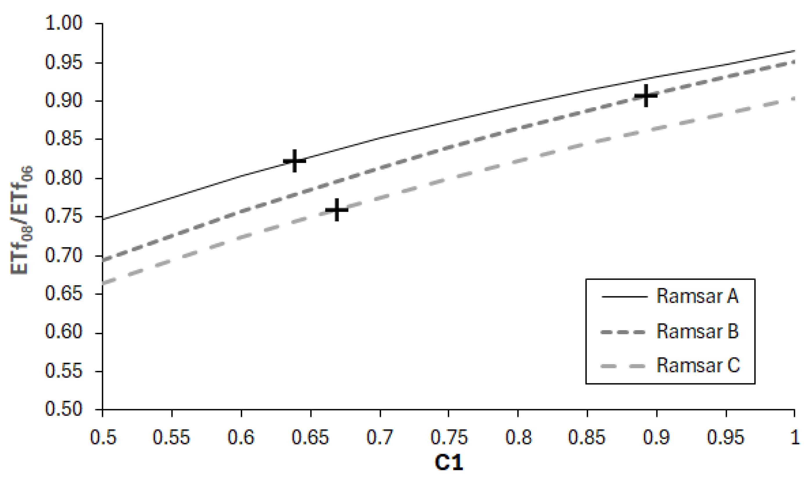
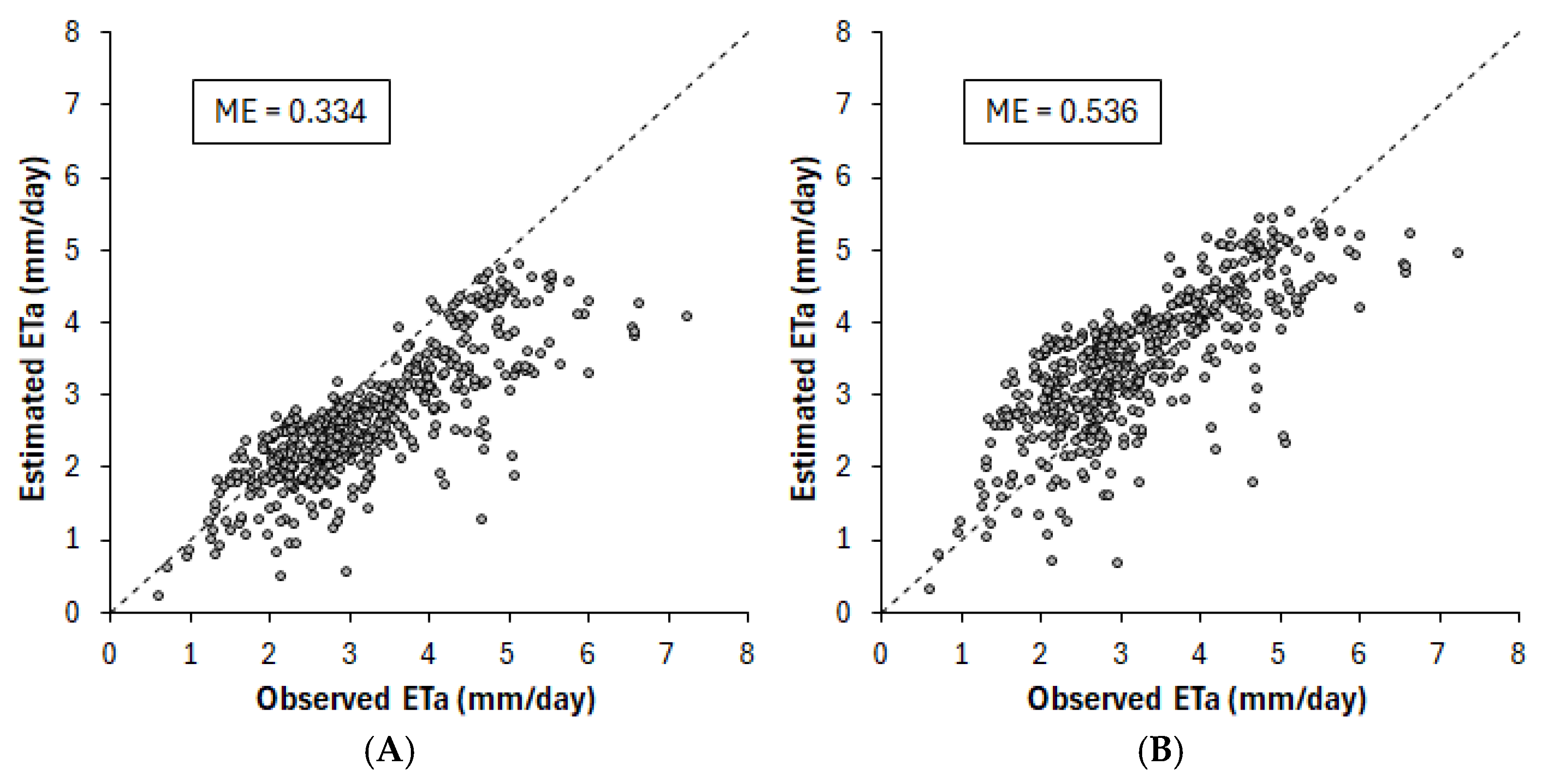
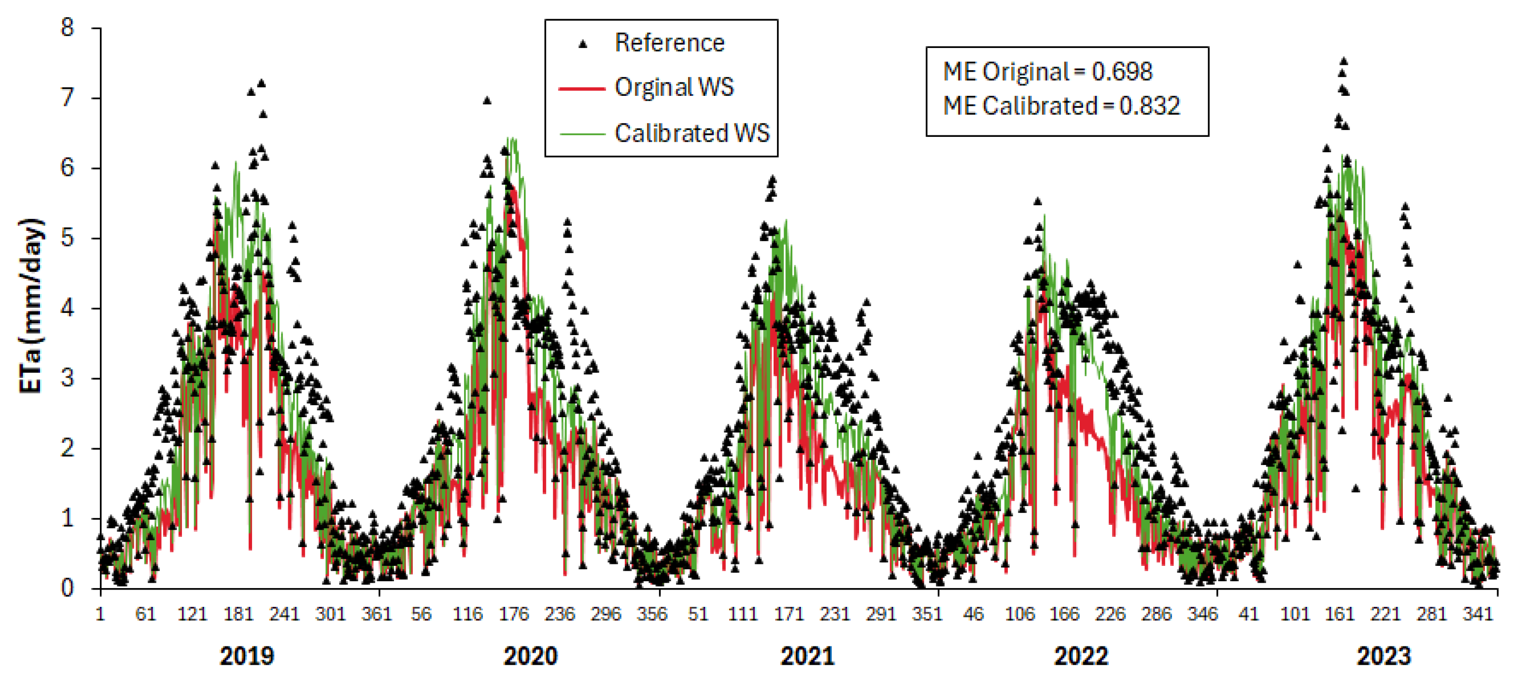
3.2. NDVI-Cws Estimates of Test Wetlands

Figure 6 shows the ETa evolution observed around the San Rossore flux tower for the years 2019–2023, which is typical of a Mediterranean coniferous forest. The average annual ETa is around 810 mm, with a peak in June followed by a slight decrease due to summer drought. The year with the lowest ETa corresponds to 2022, which is one of the driest in the last decades.

The original NDVI-Cws model clearly underestimates these values, providing an annual ETa average of around 580 mm; this issue is mostly corrected by the performed calibration, which increases this value to almost 700 mm. This pattern is confirmed by the accuracy statistics calculated for the two daily estimated ETa series: the use of the calibrated C1 and C2, in fact, increases the Nash-Sutcliff ME from 0.558 to 0.672.

The NDVI-Cws behavior is better evaluated focusing on the summer dry period, i.e., from 21st June to 21st September. The ETa estimates obtained from the two model versions considering only this period are plotted versus the respective observations in Figure 7A,B. The improvement brought by the model calibration is particularly evident: the original method strongly underestimates the ETa observations, especially for high values, and this problem is mostly corrected by the model calibration. Correspondingly, the Nash-Sutcliff ME rises from 0.334 to 0.536.

Similar results are obtained for the San Rossore grassland site; Figure 8 shows the reference ETa evolution computed by the site water balance, together with the estimates obtained by the original and the calibrated NDVI-Cws model versions. Also, in this case, the reference mean annual ETa is slightly above 800 mm and 2022 corresponds to the driest year. The general ETa pattern is better reproduced by the calibrated NDVI-Cws method, which corrects the underestimation observed when the original WS coefficients are utilized. The improvement is testified to by the Nash-Sutcliff ME, which increases from 0.698 to 0.832.

As in the previous case, a further analysis is focused on the summer dry period. Figure 9A shows the scatter plot of the ETa estimates obtained from the original model versus the respective references; Figure 9B shows the same scatter plot for the calibrated ETa estimates. Both graphs are characterized by a high dispersion around the 1:1 line, especially for high ETa values. The original model version, however, strongly underestimates the reference ETa, yielding a negative Nash-Sutcliff ME (−0.668); this problem is mostly corrected by the model calibration, which produces moderately good ETa estimates and a positive ME (0.167).

4. Discussion and Conclusions

Several remote sensing methods are currently available for ETa estimation at different spatio-temporal scales, some of which are routinely applied to provide operational products. The MODIS and LSA SAF ET products are among the most popular of these which can be used for ETa monitoring over wide regions [36]. The MODIS ET products, in fact, are provided at 500 m spatial resolution over 8-day periods, while the LSA SAF ET products are provided at 3–5 km resolution and sub-daily time step. In both cases, an issue that is particularly relevant in semi-arid Mediterranean areas concerns the reproduction of the WS impact on ETa, which is carried out relying on different principles and data sets.

Both mentioned methods do not use a full site water balance to predict the WS impact on ETa, which would be the optimal option due to the strong dependence of this process on soil water availability [37]. This methodological choice, which is justified by the common scarcity of information to drive water balances over wide areas, practically weakens the simulation of vegetation response to WS. This is particularly the case for the MODIS algorithm, which uses a meteorological variable, vapor pressure deficit (VPD), as the main down-regulator of ETa in response to WS [38]. The only indirect linkage between VPD and vegetation conditions induces a general underestimation of WS impact in areas severely affected by drought. This problem is less evident for the LSA SAF algorithm, which operates through the consideration of soil moisture estimates and yields ET products usable for drought monitoring at a regional scale [39].

The correct consideration of WS effects is also critical for the semi-empirical NDVI-Cws method, which circumvents the need for a full site water balance through the combination of meteorological and NDVI data [16]. This method separately estimates the short- and medium-term effects of WS, the former acting through rapid and reversible transpiration reduction, and the latter through more lasting green biomass decrease that is detected through NDVI reduction. Such a strategy assumes a substantial equilibrium between the two effects, which may be altered when meteorological WS is decoupled by green biomass reduction, i.e., in cases of water supply supplemental to rainfall. Maselli et al. [17] proposed a semi-empirical method to account for this possibility in irrigated croplands. The case of semi-natural vegetation fed by a shallow groundwater table can instead be addressed by the calibration approach proposed by [18], which is based on integrated LSA SAF + MODIS ETf products. This approach has been currently applied to improve ETa monitoring for all Ramsar wetlands of Tuscany, obtaining satisfactory results.

The considered indicator of WS obtained from the calibrated NDVI-Cws method, in fact, shows spatial patterns similar to those obtained from the enhanced LSA SAF ETf product. In particular, the spatial agreement between the two WS indicators is good, but the NDVI-Cws estimates show slightly higher WS impacts. These differences can be attributed to the different capacities of the two methods to reproduce WS effects in Mediterranean areas, which should be further ascertained through specific investigations. Despite being more efficient than its MODIS counterpart in simulating these effects, in fact, the actual performance of the LSA SAF ETa product in arid and semi-arid conditions is spatially and temporally variable [36]. This is partly due to the use of model drivers referring to large areas, which are locally affected by relevant uncertainty.

This problem has been currently alleviated by the selection of wide, relatively homogeneous wetlands for calibrating the NDVI-Cws method in the study region. As a result of this operation, a unique average modification was applied to the NDVI-Cws coefficients which regulate WS in all Ramsar areas of the region. The alternative use of site-specific coefficients would be theoretically more precise but would require the repetition of the calibration for each 1-km pixel and, anyway, would be constrained by this spatial resolution. Both these factors would reduce the operational applicability of the method, which is instead improved by the use of unique coefficients. The calibration of the NDVI-Cws method currently performed, in fact, allows its straightforward application at a spatial resolution that depends only on the available input datasets and can, therefore, be much higher than that of the MODIS products.

The tests of the calibrated NDVI-Cws method over two representative vegetation types, forest, and grasslands, indicate that the obtained ETa estimates are reasonably accurate. This result can be partly attributed to the combination of appropriate NDVI datasets with locally tuned drivers having comparable spatial resolution (i.e., land cover and meteorological data), which represents a major advantage of the NDVI-Cws method [16].

The currently proposed calibration of the WS coefficients for semi-natural wetlands renders the NDVI-Cws method utilizable for operational ETa monitoring also in these areas. The application of the method in other regions, however, should be preferentially preceded by a replication of the calibration process, since, as previously noted, the presence of different environmental conditions could introduce a certain variability in the optimal model configuration. In general, the obtained ETa estimates should be particularly useful in the Mediterranean as well as in other semi-arid regions, due to the model’s capacity to simulate the impact of WS at proper spatial and temporal scales. As mentioned previously, this is obviously a clear advantage over the LSA SAF and MODIS ET products, which have spatial resolution or temporal frequency suboptimal for ETa monitoring in fragmented and heterogeneous Mediterranean areas.

References

1. Allen, R.G.; Tasumi, M.; Trezza, R. Satellite-based energy balance for mapping evapotranspiration with internalized calibration METRIC model. J. Irrig. Drain. Eng. 2007, 33, 380–394. [Google Scholar] [CrossRef]
2. Tabari, H.; Talaee, P.H. Sensitivity of evapotranspiration to climatic change in different climates. Glob. Planet. Change 2014, 115, 16–23. [Google Scholar] [CrossRef]
3. Rana, G.; Katerji, N. Measurement and estimation of actual evapotranspiration in the field under Mediterranean climate: A review. Eur. J. Agron. 2000, 13, 125–153. [Google Scholar] [CrossRef]
4. Boulet, G.; Jarlan, J.; Olioso, A.; Nieto, E. Evapotranspiration in the Mediterranean region. In Water Resources in the Mediterranean Region; Elsevier: Amsterdam, The Netherlands, 2020; pp. 23–49. [Google Scholar] [CrossRef]
5. He, M.; Kimball, J.S.; Yi, Y.; Running, S.W.; Guan, K.; Moreno, A.; Wu, X.; Maneta, M. Satellite data-driven modeling of field scale evapotranspiration in croplands using the MOD16 algorithm framework. Remote Sens. Environ. 2019, 230, 111201. [Google Scholar] [CrossRef]
6. West, H.; Quinn, N.; Horswell, M. Remote sensing for drought monitoring & impact assessment: Progress, past challenges and future opportunities. Remote Sens. Environ. 2019, 232, 111251. [Google Scholar] [CrossRef]
7. Zhang, K.; Kimball, J.S.; Running, S.W. A review of remote sensing based actual evapotranspiration estimation. WIREs Water 2016, 3, 834–853. [Google Scholar] [CrossRef]
8. Liou, Y.-A.; Kar, S.K. Evapotranspiration estimation with remote sensing and various surface energy balance algorithms. A review. Energies 2014, 7, 2821–2849. [Google Scholar] [CrossRef]
9. Jones, H.G.; Sirault, X.R.R. Scaling of thermal images at different spatial resolution: The mixed pixel problem. Agronomy 2014, 4, 380–396. [Google Scholar] [CrossRef]
10. Guzinski, R.; Nieto, H.; Ramo Sánchez, R.; Sánchez, J.M.; Joma, I.; Zitouna-Chebbi, R.; Roupsard, O.; López-Urrea, R. Improving field-scale crop actual evapotranspiration monitoring with Sentinel-3, Sentinel-2, and Landsat data fusion. Int. J. Appl. Earth Obs. Geoinf. 2023, 125, 103587. [Google Scholar] [CrossRef]
11. Pereira, L.S.; Paredes, P.; López-Urrea, R.; Hunsaker, D.J.; Mota, M.; Mohammadi Shad, Z. Standard single and basal crop coefficients for vegetable crops, an update of FAO56 crop water requirements approach. Agric. Water Manag. 2021, 243, 106196. [Google Scholar] [CrossRef]
12. Maselli, F.; Papale, D.; Puletti, N.; Chirici, G.; Corona, P. Combining remote sensing and ancillary data to monitor the gross productivity of water-limited forest ecosystems. Remote Sens. Environ. 2009, 113, 657–667. [Google Scholar] [CrossRef]
13. Glenn, E.P.; Nagler, P.L.; Huete, A.R. Vegetation index methods for estimating evapotranspiration by remote sensing. Surv. Geophys. 2010, 31, 531–555. [Google Scholar] [CrossRef]
14. Senay, G.B. Modeling landscape evapotranspiration by integrating land surface phenology and a water balance algorithm. Algorithms 2008, 1, 52–68. [Google Scholar] [CrossRef]
15. Senay, G.; Kagone, S.; Parrish, G.E.L.; Khand, K.; Boiko, O.; Velpuri, N.M. Improvements and evaluation of the agro-Hydrologic VegET model for large-area water budget analysis and drought monitoring. Hydrology 2023, 10, 168. [Google Scholar] [CrossRef]
16. Maselli, F.; Papale, D.; Chiesi, M.; Matteucci, G.; Angeli, L.; Raschi, A.; Seufert, G. Operational monitoring of daily evapotranspiration by the combination of MODIS NDVI and ground meteorological data: Application and validation in Central Italy. Remote Sens. Environ. 2014, 152, 279–290. [Google Scholar] [CrossRef]
17. Maselli, F.; Battista, P.; Chiesi, M.; Rapi, B.; Angeli, L.; Fibbi, L.; Magno, R.; Gozzini, B. Use of Sentinel-2 MSI data to monitor crop irrigation in Mediterranean areas. Int. J. Appl. Earth Obs. Geoinf. 2020, 93, 102216. [Google Scholar] [CrossRef]
18. Fibbi, L.; Pieri, M.; Chiesi, M.; Gozzini, B.; Maselli, F. Integration of LSA SAF ET products and MODIS thermal infrared images for improved prediction of forest evapotranspiration. Remote Sens. Lett. 2025, 16, 400–411. [Google Scholar] [CrossRef]
19. Gardner, R.C.; Finlayson, C. Global Wetland Outlook: State of the World’s Wetlands and Their Services to People; Ramsar Convention on Wetlands; Ramsar Convention Secretariat: Gland, Switzerland, 2018; p. 88. [Google Scholar]
20. Sabbatini, S.; Mammarella, I.; Arriga, N.; Fratini, G.; Graf, A.; Hörtnagl, L.; Ibrom, A.; Longdoz, B.; Mauder, M.; Merbold, L.; et al. Eddy covariance raw data processing for CO2 and energy fluxes calculation at ICOS ecosystem stations. Int. Agrophysics 2018, 32, 495–515. [Google Scholar] [CrossRef]
21. Pastorello, G.; Trotta, C.; Canfora, E.; Chu, H.; Christianson, D.; Cheah, Y.-W.; Poindexter, C.; Chen, J.; Elbashandy, A.; Humphrey, M.; et al. The FLUXNET2015 dataset and the ONEFlux processing pipeline for eddy covariance data. Sci. Data 2020, 7, 225. [Google Scholar] [CrossRef]
22. Arriga, N.; Rannik, Ü.; Aubinet, M.; Carrara, A.; Vesala, T.; Papale, D. Experimental validation of footprint models for eddy covariance CO2 flux measurements above grassland by means of natural and artificial tracers. Agric. For. Meteorol. 2017, 242, 75–84. [Google Scholar] [CrossRef]
23. ICOS. ICOS Ecosystem Station Labelling Report. Station IT-SR2 (San Rossore 2); ICOS: Viterbo, Italy, 2019; p. 24. [Google Scholar]
24. Thornton, P.E.; Running, S.W.; White, M.A. Generating surfaces of daily meteorological variables over large regions of complex terrain. J. Hydrol. 1997, 190, 214–251. [Google Scholar] [CrossRef]
25. Fibbi, L.; Maselli, F.; Pieri, M. Improved estimation of global solar radiation over rugged terrains by the disaggregation of Satellite Applications Facility on Land Surface Analysis data (LSA SAF). Meteorol. Appl. 2020, 27, e1940. [Google Scholar] [CrossRef]
26. Didan, K.; Munoz, A.B.; Solano, R.; Huete, A. MODIS Vegetation Index User’s Guide (MOD13 Series); University of Arizona, Vegetation Index and Phenology Lab: Tucson, AZ, USA, 2015; 35p. [Google Scholar]
27. Hulley, G.; Malakar, N.; Freepartner, R. Moderate Resolution Imaging Spectroradiometer (MODIS) Land Surface Temperature and Emissivity Product (MxD21) Algorithm Theoretical Basis Document, Collection-6, JPL Publication 12-17. 2016. Available online: https://modis.gsfc.nasa.gov/data/atbd/atbd_mod21.pdf (accessed on 14 April 2024).
28. Ghilain, N.; Arboleda, A.; Gellens-Meulenberghs, F. Evapotranspiration modelling at large scale using near-real time MSG SEVIRI derived data. Hydrol. Earth Syst. Sci. 2011, 15, 771–786. [Google Scholar] [CrossRef]
29. LSA SAF 2024. Algorithm Theoretical Basis Document Evapotranspiration & Surface Fluxes (DMETV3). EUMETSAT LSA SAF, Product LSA-312v.3, Document No. SAF/LAND/RMI/ATBD/METv3/1.0, Issue 2. Available online: https://nextcloud.lsasvcs.ipma.pt/s/7QLcZfABg5H6mkq?dir=/ATBD-Algorithm_Theoretial_Basis_Document (accessed on 10 January 2025).
30. Jensen, M.E.; Haise, H.R. Estimating evapotranspiration from solar radiation. J. Irrig. Drain. Div. ASCE 1963, 89, 15–41. [Google Scholar] [CrossRef]
31. Gutman, G.; Ignatov, A. The derivation of the green vegetation fraction from NOAA/AVHRR data for use in numerical weather prediction models. Int. J. Remote Sens. 1998, 19, 1533–1543. [Google Scholar] [CrossRef]
32. Fibbi, L.; Pieri, M.; Chiesi, M.; Maselli, F. Use of LSA-SAF products to improve the operational estimation of forest evapotranspiration. J. Appl. Remote Sens. 2023, 17, 034503. [Google Scholar] [CrossRef]
33. Senay, G.B.; Friedrichs, M.K.; Moron, C.; Parrish, G.E.L.; Schauer, M.; Khand, K.; Kagone, S.; Boiko, O.; Huntington, J. Mapping actual evapotranspiration using Landsat for the conterminous United States: Google Earth Engine implementation and assessment of the SSEBop model. Remote Sens. Environ. 2022, 275, 13011. [Google Scholar] [CrossRef]
34. Nash, J.E.; Sutcliffe, J.V. River flow forecasting through conceptual models part I—A discussion of principles. J. Hydrol. 1970, 10, 282–290. [Google Scholar] [CrossRef]
35. Allen, R.G. Using the FAO-56 dual crop coefficient method over an irrigated region as part of an evapotranspiration intercomparison study. J. Hydrol. 2000, 229, 27–41. [Google Scholar] [CrossRef]
36. Hu, G.; Jia, L.; Menenti, M. Comparison of MOD16 and LSA-SAF MSG evapotranspiration products over Europe for 2011. Remote Sens. Environ. 2015, 156, 510–526. [Google Scholar] [CrossRef]
37. Teuling, A.J.; Seneviratne, S.I.; Williams, C.; Troch, P.A. Observed timescales of evapotranspiration response to soil moisture. Geophys. Res. Lett. 2006, 33, L23403. [Google Scholar] [CrossRef]
38. Mu, Q.; Zhao, M.; Running, S.W. Improvements to a MODIS global terrestrial evapotranspiration algorithm. Remote Sens. Environ. 2011, 115, 1781–1800. [Google Scholar] [CrossRef]
39. Sepulcre-Canto, G.; Vogt, J.; Arboleda, A.; Antofie, T. Assessment of the EUMETSAT LSA-SAF evapotranspiration product for drought monitoring in Europe. Int. J. Appl. Earth Obs. Geoinf. 2014, 30, 190–202. [Google Scholar] [CrossRef]
Figure 1. CORINE land cover categories of Tuscany defined as in [18], with superimposed Ramsar areas; the three areas chosen for model calibration are Fucecchio (A), Migliarino (B), and San Rossore (C). The lower left box shows the position of Tuscany in Italy, while the upper box indicates the location of the two test sites in the San Rossore area (1 = forest, 2 = grassland).
Hydrology 12 00139 g001
Figure 2. Mean ratio ETf08/ETf06 estimated as described in [18].
Hydrology 12 00139 g002
Figure 3. Mean ratios ETf08/ETf06 of the five CLC categories and Ramsar areas obtained from the LSA SAF + LST products and NDVI-Cws estimates (see text for details).
Hydrology 12 00139 g003
Figure 4. ETf08/ETf06 ratios simulated for varying C1 values in the three selected Ramsar areas with indication of the optimum ratios and corresponding C1s identified from the integrated LSA SAF + MODIS ETf product (crosses).
Hydrology 12 00139 g004
Figure 5. Mean ETf08/ETf06 ratios obtained by the NDVI-Cws method.
Hydrology 12 00139 g005
Figure 6. ETa evolutions observed and estimated by the original and calibrated NDVI-Cws versions at the San Rossore pine forest site.
Hydrology 12 00139 g006
Figure 7. Scatter plots of summer ETa observed and estimated by the original (A) and the calibrated (B) model versions at the San Rossore pine forest site.
Hydrology 12 00139 g007
Figure 8. ETa evolutions obtained from the site water balance and estimated by the original and the calibrated NDVI-Cws model versions at the San Rossore grassland site.
Hydrology 12 00139 g008
Figure 9. Scatter plots of summer ETa obtained from the site water balance and estimated by the original (A) and the calibrated (B) model versions at the San Rossore grassland site.
Hydrology 12 00139 g009