Impact of Precipitation Uncertainty on Flood Hazard Assessment in the Oueme River Basin

Abstract

This study evaluates the impact of precipitation ensembles on flood hazards in the Ouémé River Basin by coupling the hydrological HBV and hydrodynamic HEC–RAS model. Both models were calibrated and validated to simulate hydrological and hydraulic processes. Meteorological and hydrometric data from 1994 to 2016, along with flood maps and DEM are used. Evapotranspiration data are calculated using Hargreaves–Samani formula. The coupling HBV–HEC–RAS models enabled the generation of ensemble hydrographs, flood maps, flood probability maps and additional statistics in West Africa for the first time, offering a comprehensive understanding of flood dynamics under uncertainty. Ensemble hydrographs and maps obtained enhance decision-making by showing discharge scenarios, spatial flood variability, prediction reliability, and probabilities, supporting targeted flood management and resource planning under uncertainty. The findings underline the need for a comprehensive strategy to mitigate both common and rare flood events while accounting for spatial uncertainties inherent in hydrological and hydraulic modeling.

1. Introduction

Flooding is a major hazard in West Africa, causing severe damage and putting large numbers of the African population at risk [1,2,3,4]. In the Guinean coastal zone, the increasing population density and urbanization aggravate flood exposure and vulnerability, and hence, flood risk [5,6]. In addition, the river basins in West Africa are characterized by high hydro-climatic variability [2], such as the Ouémé river basin in Benin, where frequent flood events of different magnitudes were observed [7]. Managing the risk of flood hazards and the hydro-climatic variability in West Africa necessitates a reliable hazard assessment, prediction, and mitigation. Models such as hydrological and hydrodynamic models are widely used to quantify and understand flooding for flood risk management. Thus, hydrologic models are used for the rainfall-runoff modeling in the catchment, where the modeled output (discharges) is used as inputs for hydrodynamic models (inflows). Hydrodynamic models facilitate an accurate computation of the flood routing in the stream and the precise calculation of water levels and the spatial extent of the flood event. These models are thus essential tools for decision-makers and practitioners in many regions of the world. One hydrodynamic model widely used in West Africa is the HEC–RAS model [8,9,10,11,12].

Yet, flood modeling is subject to various uncertainties [13,14] that need to be accounted for in hazard quantification and decision-making. Generally, uncertainties in flood modeling can be categorized into model assumption uncertainties, parameter estimation uncertainties, and model input uncertainties [15]. Although uncertainty quantification is now well established in weather and flood forecasting [16,17], such approaches are rarely applied to flood hazard modeling, especially in data-poor regions such as West Africa. In the past, the first efforts were made to account for these sources of uncertainty in hydrology, for example, by [18]. They used the Generalized Likelihood Uncertainty Estimation (GLUE) method to quantify the uncertainties of different hydrological models in selected river basins of West Africa. Modeling techniques, such as Bayesian model averaging, were explored and applied by [19] to address the model uncertainties in data-scarce river basins. It is, however, commonly understood that model input uncertainty, i.e., the precipitation input, is the main contributor to uncertainties in flood modeling [20,21]. This uncertainty is especially pronounced by the spatial variability of precipitation [22]. To assess the uncertainty of flood modeling, precipitation ensembles were used in various flood studies (e.g., [23,24]). In the Ouémé River basin, ref. [25] moreover investigated the impacts of uncertainties linked to a random component of rainfall using the least action principle.

However, these studies on flooding in West Africa focused only on discharge estimation, whereas the computation of flood extents was not considered. In the present study, we propose a modeling framework to account for the challenges of flood hazard evaluation in West Africa using the Ouémé river as a case study. In this study, we address how large flood maps for extreme events differ when precipitation uncertainty is considered using stochastic simulation techniques for ensemble generation. Moreover, we assess whether a single precipitation input from interpolation technique is already sufficient information for comprehensive flood modeling in comparison to the ensemble-based approach. Moreover, our framework aims to highlight what decision-makers and practitioners can expect for flood maps if multiple precipitation ensembles are used for flood management analysis.

For these purposes, we apply a coupled modeling approach to evaluate the flood hazard for the Ouémé river basin in Benin using precipitation and discharge ensembles. The precipitation ensembles are stochastically derived from in situ data to maintain the rainfall variability in this region. We use the hydrological model Hydrologiska Byråns Vattenbalansavdelning (HBV) model [26,27] to generate discharge ensembles as inflows for the flood model HEC–RAS [28]. Applying the HEC–RAS model then allows the quantification of accurate flood extents and flood maps. To the best of our knowledge, a coupling of hydrological and hydrodynamic models and the application of precipitation ensembles for flood map investigation have not been applied yet in West Africa.

In the following, we first present the methodology applied, the datasets and models used, and how the models are set up and evaluated. Then, the results are shown, the methodology is discussed, and last, we conclude the paper with the major findings of this study.

2. Materials and Methods

Figure 1 gives an overview of the methodology applied in this study to evaluate precipitation ensembles on flood hazard. Precipitation ensembles were first generated by stochastic geostatistical simulation technique based on the Spectral Turning Bands Method (STBM). These precipitation ensembles were then used as input in the hydrological HBV model for simulating discharges. These discharges served inflows to the hydrodynamic HEC–RAS–1D model for simulating discharges and flood maps. This methodology is explained in more detail in the following.

2.1. Study Site and Datasets

2.1.1. Study Site

The study area, the Ouémé basin, is located in Republic of Benin, West Africa. Benin is geographically situated between 06°25′ to 12°30′ northern latitude and 01°00′ to 03°40′ eastern longitude (Figure 2). It is bordered to the north by Niger, to the northwest by Burkina Faso, to the west by Togo, to the east by Nigeria, and to the south by the Gulf of Guinea. Benin is located entirely in the tropical sub-Saharan region. The Ouémé river rises in the Atacora massif in northwestern Benin and has two main affluents: the Okpara and the Zou. The Ouémé basin at the Bonou gauge is about 50,000 km², and the river length is around 500 km [8].

The catchment is mainly characterized by the Precambrian basement. It consists predominantly of complex migmatites granulites and gneisses, including less abundant mica shists, quartzites, and amphibolites [29]. The Ouémé Basin is characterized by four major soil types [30]. In its northern and center parts, there are mostly crystalline base soils; in its southern part, the soils are the hydromorphic Vertisols, the sand-stone plain and the quartz rich sand.

There are three climatic zones in the Ouémé River basin [30,31]. North Ouémé endures a unimodal rainfall regime with a rainy season from May to October and a dry season from November to March. In middle Ouémé, a transitional rainfall regime prevails with a rainy season from March to October, with or without a small dry season during August [32]. The southern Ouémé River basin endures a bimodal rainfall regime with two wet seasons (a long one between March and July and a short one between September and mid-November) and two dry seasons (a long one between November and March and a short one in August).

2.1.2. Datasets

The data used in this work are summarized in

Table 1. Data used in this study.

Data	Period	Source
Daily precipitation	1994–2016	CS-STBM [33]
Daily air temperature	1994–2016	Météo Bénin, ERA5
Daily discharge	1994–2016	DGEau, Benin
Daily water level	2011–2016	DG Eau, Benin
Flood maps	October 2016	SENTINEL-1
DEM	-	Copernicus-GLO30
Rating curve	2011–2016	DG Eau, Benin

. The precipitation data are gridded data generated by stochastic geostatistical simulation technique based on the Spectral Turning Bands Method (STBM) [33]. The air temperature data are provided by Météo Bénin for the Bétérou and Savè subcatchments. ERA5 re-analysis data [34] are used for the Kaboua, Atchérigbé, Zangnanado, and Bonou subcatchments. The discharge and water level data are obtained from Direction Générale de l’Eau (DGEau) for the Bétérou, Savè, Kaboua, Atchérigbé, Zangnanado, and Bonou gauges. We selected the best overlap from the input data for the modeling in the present study (from 1994 to 2016). The completeness and spatial consistency of meteorological and hydrometric datasets, spanning the period 1994–2016, were rigorously evaluated. A detailed analysis of precipitation data quality is provided in [33]. As illustrated in Figure A1 (Appendix A), discharge data availability across all monitoring stations averaged 82.31% during the study period (1994–2016), reflecting a high degree of temporal coverage despite localized gaps. The simulation period for the hydrological modeling is split into three periods: a warming up period (1994), a calibration period from 1995 to 2004, and a validation period from 2005 to 2014. For the hydrodynamic–numerical modeling, the simulation period covers the years between 2011 and 2016.

2.2. Precipitation Estimation

To improve the reliability of hydrological modeling, we addressed uncertainty in rainfall input by using two rainfall products: a reference dataset created through nearest-neighbor interpolation (“Reference”) and a stochastic ensemble of 20 simulated rainfall scenarios generated with the Conditional Simulation with Spectral Turning Bands Method (CS-STBM, “simulation”). The Reference dataset provides a deterministic baseline estimation of rainfall, while the simulation ensemble captures broader spatial variability, accounting for uncertainties that standard interpolation methods cannot represent [35].

Following the methodology detailed in [33], we configured the CS-STBM with an isotropic variogram (30 km range, no nugget effect) and regionalized the in situ observations to a 0.05° grid (approximately 5 km). The spatial distribution of the rain gauges used for both the interpolation and the conditional simulation is shown in Figure 1 of [33], which provides an overview of the station network across the study region. The generated rainfall fields were then spatially averaged over each sub-catchment. This approach yielded six spatialized time series representing key aspects of rainfall variability across each catchment, which were then used as inputs in the coupled HBV–HEC–RAS model setup to simulate discharge and flood inundation.

Based on this rainfall modeling approach, we gain insights into the impact of rainfall uncertainty on hydrological and hydraulic model outputs.

2.3. Models

2.3.1. The HBV Model

The HBV (Hydrologiska Byråns Vattenbalansavdelning) hydrological model [26,27] is a global conceptual model on the catchment scale. In 1996, the HBV light version was created [27]. The HBV model simulates daily flow using daily temperature, precipitation and an estimate of potential evapotranspiration as input data. Despite its relatively simple structure, the HBV model works well and continues to be used by a large number of scientists around 50 years after its first use [36]. Integrating conceptual models like HBV with climate projections offers a robust tool for managing uncertainties in future water availability and flood risks [37,38,39]. Within its structure, the model has fifteen parameters constituting the different routines (Figure 3). These routines are the following: the snow routine, the soil moisture routine, the response function, and the routing routine. The parameters within the different routines are summarised in

Table 2. HBV model parameters in the different routines.

Parameter	Explanation	Unit
Snow routine
TT	Threshold temperature	°C
CFMAX	Degree-Δt factor	mm °C−1Δt −1
SFCF	Snowfall correction factor	-
CWH	Water holding capacity of snow	-
CFR	Refreezing coefficient	-
SP	Seasonal variability in degree-Δt factor	-
Soil moisture routine
FC	Field capacity: Maximum soil moisture storage	mm
LP	Soil moisture value above which AET reaches PET	-
BETA	Shape coefficient	-
Response routine
K0	Additional recession coefficient of upper groundwater store	Δt −1
K1	Recession coefficient of upper groundwater store	Δt −1
K2	Recession coefficient of lower groundwater store	Δt −1
UZL	threshold parameter for K0 outflow	mm
PERC	Threshold parameter	mm Δt −1
Routing routine
MAXBAS	Length of equilateral triangular weighting function	mm Δt −1

. Given that there is no snow in Benin, the snow module was deactivated in the model setting up. The evapotranspiration data are calculated for the same periods using the Hargreaves–Samani formula [40,41] shown by Equations (1) and (2):

ET_r = 0.0135R_S(T_mean + 17.8)

(1)

R_S = 0.16R_a(T_max – T_min)^0.5,

(2)

where ET_r is the reference evapotranspiration in a given time period (day, month), T_max (°C), the mean maximum air temperature, T_min (°C), the mean minimum air temperature, and the incoming short-wave solar radiation, R_S, in the considered period (mm/d), R_a, is the extraterrestrial radiation.

2.3.2. The HEC–RAS Model

The HEC–RAS model is a hydraulic numerical model developed by the US Army Corps of Engineers [28]. The application of the model facilitates the computation of flood routing in the river channel and the inundation extents. In HEC–RAS, the computational domain of the river is spatially discretized into user-defined cross sections. Between adjacent cross sections, the mass and momentum conservation (so-called “Saint Venant equations”) are calculated. The conservation of mass is computed as

$${\displaystyle \frac{\partial \mathrm{Q}}{\partial \mathrm{x}}}+{\displaystyle \frac{\partial \mathrm{A}}{\partial \mathrm{t}}}=0.$$

(3)

And the conservation of momentum is described with

$${\displaystyle \frac{1}{\mathrm{A}}}{\displaystyle \frac{\partial \mathrm{Q}}{\partial \mathrm{t}}}+{\displaystyle \frac{1}{\mathrm{A}}}{\displaystyle \frac{\partial \left(\raisebox{1ex}{${\mathrm{Q}}^2$}\!\left/ \!\raisebox{-1ex}{$\mathrm{A}$}\right.\right)}{\partial \mathrm{t}}}+\mathrm{g}{\displaystyle \frac{\partial \mathrm{h}}{\partial \mathrm{x}}}-\mathrm{g}\left({\mathrm{S}}_0-{\mathrm{S}}_{\mathrm{f}}\right)=0,$$

(4)

where Q is the discharge, A is the cross-section area, t represents time, g is the gravitational acceleration, h is the flow depth, S₀ is the channel bed slope, and S_f is the friction slope. In HEC–RAS, numerical approximations are used to solve the Saint Venant Equations. The flow discharge Q and the flow depth h are computed for every cross section at each time step.

The HEC–RAS model requires geospatial information for the modeling domain, including topographic data, channel geometry, and land cover data. We use the DEM data from Copernicus-GLO30 to delineate the floodplains and river profiles. The length of the river reach analyzed is 320 km. The spacing of the cross sections is 150 m. The river width (bank lines) is estimated from Google Earth imagery. Figure A2 give an exemplary cross section in the HEC–-RAS model of the Ouémé river and the riverbed geometry of this cross section. We postulate that the satellite-based DEM data are reliable for all spatial regions apart from where the bankfull river water is impairing the remote sensing. Hence, the elevation of each point in between the bank lines is subject to adjustment, i.e., calibration. The roughness parameter is represented by the Manning’s value to account for the land cover in HEC–RAS. The mean flow velocity v_m is computed based on the Gauckler–Manning–Strickler equation using the hydraulic radius R and the energy slope I:

$${\mathrm{v}}_{\mathrm{m}}={\displaystyle \frac{1}{\mathrm{n}}}·{\mathrm{R}}^{2/3}·{\mathrm{I}}^{1/2}.$$

(5)

The roughness parametrization is separated for the main stream and the floodplains and requires calibration. The observed discharge and water level data at the gauging station of Bonou are used for calibration and validation. The model calibration consists of two steps. First, the river bed geometry in between the bank lines is adjusted with steady-state simulations to fit the modeled to the observed rating curve at Bonou. Second, the roughness parameters for the mainstream and the floodplains are calibrated with unsteady-state simulations to fit the modeled to the observed discharge time series at Bonou. The model validation is applied for additional flow events and compares the modeled flood inundation extent with observed flood maps from the SENTINEL-1A mission.

2.3.3. Model Evaluation Criteria

The HBV model is calibrated for a better reproduction of the observations in the Ouémé basin. The calibration is conducted by adjusting automatically (by GAP optimization and Monte Carlo tools offered in HBV-light) and manually the parameters in order to have the best fitting possible between simulated and observed flows. The objective functions used in this work are the Nash–Sutcliffe efficiency coefficient (NSE) [44,45], the Kling and Gupta coefficient (KGE) [45,46], the coefficient of determination (R²) [44,47], and the volume error (Vol-Eff) [44] that the equations are following:

$$\mathrm{N}\mathrm{S}\mathrm{E}=1-{\displaystyle \frac{\sum _{\mathrm{i}=1}^{\mathrm{n}}{\left({\mathrm{Q}}_{\mathrm{o}\mathrm{b}\mathrm{s}\mathrm{i}}-{\mathrm{Q}}_{\mathrm{s}\mathrm{i}\mathrm{m}\mathrm{i}}\right)}^2}{\sum _{\mathrm{i}=1}^{\mathrm{n}}{\left({\mathrm{Q}}_{\mathrm{o}\mathrm{b}\mathrm{s}\mathrm{i}}-{\overline{\mathrm{Q}}}_{\mathrm{o}\mathrm{b}\mathrm{s}\mathrm{i}}\right)}^2}}$$

(6)

$$\mathrm{K}\mathrm{G}\mathrm{E}=1-\sqrt{{\left(\mathrm{r}-1\right)}^2+{\left(\mathsf{\alpha }-1\right)}^2{+\left(\mathsf{\delta }-1\right)}^2}$$

(7)

$${\mathrm{R}}^2={\displaystyle \frac{(\sum _{\mathrm{i}=1}^{\mathrm{n}}{\left({\mathrm{Q}}_{\mathrm{o}\mathrm{b}\mathrm{s}\mathrm{i}}-\overline{{\mathrm{Q}}_{\mathrm{o}\mathrm{b}\mathrm{s}\mathrm{i}}}\right)\left({\mathrm{Q}}_{\mathrm{s}\mathrm{i}\mathrm{m}\mathrm{i}}-\overline{{\mathrm{Q}}_{\mathrm{s}\mathrm{i}\mathrm{m}\mathrm{i}}}\right))}^2}{\sum _{\mathrm{i}=1}^{\mathrm{n}}{\left({\mathrm{Q}}_{\mathrm{o}\mathrm{b}\mathrm{s}\mathrm{i}}-\overline{{\mathrm{Q}}_{\mathrm{o}\mathrm{b}\mathrm{s}\mathrm{i}}}\right)}^2\sum _{\mathrm{i}=1}^{\mathrm{n}}{\left({\mathrm{Q}}_{\mathrm{s}\mathrm{i}\mathrm{m}\mathrm{i}}-\overline{{\mathrm{Q}}_{\mathrm{s}\mathrm{i}\mathrm{m}\mathrm{i}}}\right))}^2}}$$

(8)

$$\mathrm{Vol}-\mathrm{Eff}=1-{\displaystyle \frac{\left|\sum _{\mathrm{i}=1}^{\mathrm{n}}\left({\mathrm{Q}}_{\mathrm{o}\mathrm{b}\mathrm{s}\mathrm{i}}-{\mathrm{Q}}_{\mathrm{s}\mathrm{i}\mathrm{m}\mathrm{i}}\right)\right|}{\sum _{\mathrm{i}=1}^{\mathrm{n}}\left({\mathrm{Q}}_{\mathrm{o}\mathrm{b}\mathrm{s}\mathrm{i}}\right)}},$$

(9)

where r is the linear correlation coefficient between observed and simulated discharge, $\alpha$ is the ratio of the standard deviation of the simulated discharge over the standard deviation of the observed discharge, $\delta$ is the ratio of the mean simulated discharge over the mean observed discharge, ${\mathrm{Q}}_{\mathrm{o}\mathrm{b}\mathrm{s}\mathrm{i}}$ is the observe discharge, ${\mathrm{Q}}_{\mathrm{s}\mathrm{i}\mathrm{m}\mathrm{i}}$ is the simulated discharge, $\overline{{\mathrm{Q}}_{\mathrm{s}\mathrm{i}\mathrm{m}\mathrm{i}}}$ is the mean simulated discharge, and i is the number of time steps. These criteria are the most commonly used in hydrology [48]. The calibration is good if the objective functions are all greater than 0.5 and the fitting is perfect if the values are as close as possible to 1 [49]. Sensitivity analysis is applied in order to improve the calibration. Once the calibration has been carried out, the set of optimal parameters is used to run the model over another period for validation.

For the evaluation of the HEC–RAS modeling, the rating curves derived at the gauge of Bonou are used. The rating curves can include uncertainties [1,50]. Hence, we add 95%-confidence intervals based as suggested by [1]. A robust performance is achieved when the simulated rating curve is within the confidence interval. The performance of predicting the flood inundation with HEC–RAS is quantified with the Pierce skill score (PSS) [51]. The fit of the simulated to the observed flood extent with the PSS compares modeled hit rate with the overprediction of the model:

$$\mathrm{P}\mathrm{S}\mathrm{S}={\displaystyle \frac{\mathrm{A}}{\mathrm{A}+\mathrm{C}}}-{\displaystyle \frac{\mathrm{B}}{\mathrm{B}+\mathrm{D}}}$$

(10)

where A, B, C, and D are read from the contingency table (

Table 3. Contingency table summarizing the cells being classified as correct and over- or under-predicted.

	Simulated Flooded	Simulated Not Flooded
Observed flooded	A (correct flooding)	C (under-prediction)
Observed not flooded	B (over-prediction)	D (correct dry)

). The PSS ranges from 0 to 1, where a value of 1 indicates a perfect fit. The contingency table counts the raster pixels, whether they are flooded in the model or not, and compares whether the raster pixel is inundated in the observation. As the observed data, we used the flood map derived from the SENTINEL-1 mission from October 2016 for the area around the gauge of Bonou.

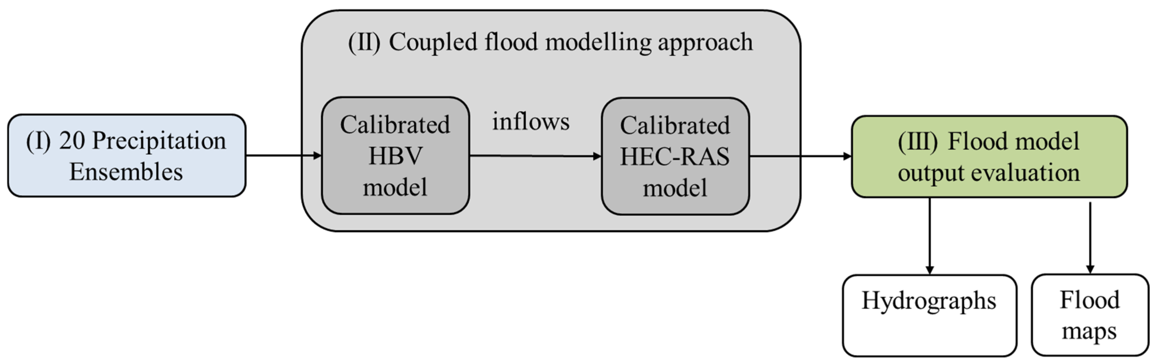
2.3.4. Coupling HBV–HEC–RAS

This work focused on the uncertainty linked to the precipitation data. The methodology used in this study allows to estimate the uncertainty in two ways from the precipitation scenarios and the coupling of the two models. One (1) is to use the discharges from the coupling and the other (2) is based on the analysis of the differences observed across the different flood maps. To run, the HEC–RAS model needs, as boundary conditions, the flow hydrograph at the Bétérou gauge (the upstream), the lateral inflow hydrographs at tributaries (Savè1, Savè2, Savè3, Savè4, Okpara, and Zou (Figure 4)) and the normal depth at the outlet (Bonou). The observed discharge data at the Bétérou outlet are used as an inflow boundary condition upstream. There is no streamflow measured directly at the outlets of the tributaries. These flows were simulated with HBV. Spatial precipitation data were generated for the sub-basins of these tributaries and used as inputs for the calibrated and validated HBV model. The outputs of the HBV model are used as inputs for the HEC–RAS hydrodynamic model. This coupling provides simulated discharge at Bonou, flood maps with water levels, and flood extents. To apply this methodology, twenty (20) precipitation patterns were generated stochastically. These precipitation patterns, as well as the spatialization of the actual precipitation termed “Reference”, were used in the HBV–HEC–RAS coupling for the year 2011. Twenty simulated discharges (Q_sim) were then obtained, plus the Reference flows (Q_Ref) and the flood maps. A comparison was carried out between Q_HBV, Q_Ref, their average Q_Mean_Ref_HBV, and the observations Qobs to see the advantage from the coupling and the possible use of the prediction average. For the approach, (1) the 20 simulated discharges were plotted in the same graphic as well as the observation (Q_obs) and Q_Ref curves to constitute the discharge ensembles. The two statistic descriptions, r-factor and p-factor, were calculated. For the approach, (2) flood maps were computed for the twenty scenarios as well as the Reference. The Mean, the Maximum, the Standard Deviation, the flood occurrence and the flood probability maps were computed for making comparison and finding out the difference in flood extent and flood level. This is a conceptual approach to estimate the uncertainty in modeling.

3. Results

3.1. Model Evaluation

3.1.1. Calibration and Validation of HBV Model

The HBV model is calibrated and validated with six gauging stations.

Table 4. Model efficiency for calibration period (1995–2004) in Ouémé.

Eff.	Bétérou	Savè	Kaboua	Atchérigbé	Zangnanado	Bonou
KGE	0.83	0.73	0.80	0.61	0.88	0.91
NSE	0.86	0.85	0.78	0.62	0.87	0.90
NSE-SS	0.79	0.77	0.71	0.46	0.80	0.82
R2	0.87	0.88	0.79	0.64	0.87	0.91
Vol-Eff.	0.93	0.85	0.85	0.98	0.94	0.95

and

Table 5. Model efficiency for validation period (2005–2014) in Ouémé.

Eff.	Bétérou	Savè	Kaboua	Atchérigbé	Zangnanado	Bonou
KGE	0.77	0.61	0.82	0.60	0.90	0.64
NSE	0.80	0.76	0.86	0.51	0.89	0.77
NSE-SS	0.73	0.66	0.81	0.42	0.83	0.63
R2	0.81	0.82	0.86	0.54	0.89	0.90
Vol-Eff.	0.98	0.77	0.86	0.72	0.95	0.75

show the criteria values over the Ouémé catchment. NSE-SS indicates the NSE for specified season (high flows period). As shown in these tables, very satisfactory results have been obtained in calibration as well as in the validation period. For the calibration period, Bonou has the best model performance among subcatchments with 0.91, 0.90, 0.82, 0.91 and 0.95, respectively, for KGE, NSE, NSE-SS, R² and Vol-Eff. Atchérigbé is the least satisfactory with 0.61, 0.62, 0.46 and 0.64, respectively, for KGE, NSE, NSE-SS, R² but has the best Vol-Eff value with 0.98. For the validation period, Zangnanado is the best subcatchment in performance with 0.90, 0.89, 0.83, 0.89 and 0.95, respectively, for KGE, NSE, NSE-SS, R² and Vol-Eff. Atchérigbé is still the least satisfactory but acceptable, except NSE-SS (KGE: 0.60, NSE: 0.51, NSE-SS: 0.42, R²: 0.54, Vol-Eff: 0.72). Bonou has dropped in most criteria. The model performance has improved in Kaboua and experienced a slight decline in Savè. In most years, the observed and simulated discharges align well during peak flow periods, showing a good agreement between the timing of high flows. It should also be noted that the model occasionally overestimated peak discharges in Bonou subcatchment in calibration period (1995, 1999, 2003) as well as in the validation period (2008, 2010, 2014) (Figure 5). During dry seasons, the model aligns well with the observed flow.

3.1.2. Performance Evaluation of the HEC–RAS Model

The calibrated and observed rating curve for the gauge of Bonou is shown in Figure 6. The calibrated rating curve is similar to the observed rating curve and fully lies within the range of the confidence intervals. Low, medium, and high flows fit well with the calibrated HEC–RAS model. The roughness parameters are calibrated with unsteady-state simulations where the years 2011, 2012, 2014, and 2016 are considered. These four years were selected because the data quality, e.g., the number of missing data points, is acceptable. The model efficiency of the HEC–RAS–1D model for each year is given in

Table 6. Model efficiency of the HEC–RAS model for validation.

Eff.	2011	2012	2014	2016	Mean of All Years
KGE	0.78	0.50	0.72	0.75	0.69
NSE	0.72	−0.10	0.74	0.76	0.53
R2	0.72	0.50	0.78	0.77	0.69

. Overall, the model performs well with mean values for KGE of 0.69, for NSE of 0.53, and for R² of 0.69. The poor NSE fit for 2012 is explained with the temporal mismatch of the flood peaks. The discharge time series and the rating curve of the unsteady runs are shown in Appendix A, Figure A3.

A comparison with the flood extent derived from SENTINEL-1 is used not only to validate the model pointwise for the gauging station of Bonou but also to determine the model performance to predict the flood extent. Figure 7 shows the overlap of the HEC–RAS flood model with the SENTINEL-1 flood mask for October 2016. The computed PSS value is 0.86 indicating a good performance of the HEC–RAS model. Overall, the applied HEC–RAS model is capable to predict both the discharge at the gauge of Bonou (e.g., mean NSE = 0.53) and the flood extent (PSS = 0.86).

3.2. Implications of Precipitation Ensembles on Discharge and Flood Map Modeling

3.2.1. Discharge Comparison

The simulated discharges (Q_HBV, Q_Ref, Q_mean, HBV_Ref) are similar to the observed discharge data Qobs. An increasing discharge from July, peaking around October, and then decreasing in December (Figure 8) can be observed. Q_HBV and Q_Ref show good alignment with Qobs, but there are periods where the predictions deviate from the observed data. For example, from late October to early November, Qobs is below Q_HBV and Q_Ref, indicating an overestimation by the models. The HBV model (Q_HBV) tends to slightly overestimate flow relative to observed values and lags in predicting event occurrence, while the Reference model (Q_Ref) occasionally overestimates during peak flow periods and provides a better temporal fit with Qobs. Q_Mean_HBV_Ref serves as a balance between the two predictions, averaging the strengths and weaknesses of Q_HBV and Q_Ref. It provides a reasonable estimate for periods of more moderate flow, but struggles to reproduce extremes (high or low flows) and lags in predicting event occurrence.

3.2.2. Use of the Flow Rates Resulting from the Coupling of the Two Models

The simulated hydrographs (Qsim_0 to Qsim_19) represent a range of discharges whose dispersion indicates the uncertainty in the model predictions (Figure 9). This dispersion is greater during periods of higher discharge, particularly during the peak around October, and is much reduced during periods of low discharge (July and late November). The observed discharge (Qobs) is generally within the range of the simulated values, but there are cases where it deviates, as is the case in September where it is lower than most of the simulated values. The variability between simulations highlights the importance of considering several scenarios in hydrological modeling to capture the full range of possible outcomes. Overall, the observed data are within the band of the simulations. Determination of the statistical quantities, r-factor and p-factor calculated give r-factor = 0.60 and p-factor = 0.45. These results, more or less acceptable, show the capacity of the model to predict real conditions, despite the inherent uncertainties.

3.2.3. Use of Flood Maps for Uncertainty Estimation

Ensembles Maps

In the following, the spatial variability of flow depth across the twenty ensemble scenarios (Ensembles 0 to 19) along the Ouémé River is discussed. Figure 10 shows the flood maps for scenarios 0 to 3, flood maps for scenarios 4 to 19 are presented in Figure A4, Figure A5, Figure A6 and Figure A7 in the Appendix B. The analysis focused only on the lower part of the river (Lower Ouémé) flowing through the communes of Zangnanado, Ouinhi, Zogbodomè, Zè and Bonou as in the upper part the differences are minor. The general shape and flow of the river remain consistent across all ensembles. There are areas where the depth agrees across all ensembles such as the upper and lower sections of the Lower Ouémé indicating high certainty in the depth predictions. Depth variability is observed, particularly in the middle sections of the Lower Ouémé, indicating uncertainty in the model predictions. For example, some sets show large areas of deeper water (red and brown areas) compared to others, which show these areas as shallower (blue or yellow). The observations from these sets (0 to 3 in Figure 10) are similar to the maps in the Appendix B.

Uncertainty Analysis Through Statistic Descriptions

The Reference, Mean, Maximum, and Standard Deviation have been used in this chapter to highlight the consistency or variability in depth predictions across ensembles. The “Reference” map serves as a reference or control for comparison. It represents a specific model output, the standard prediction. The “Mean” map displays the average depth calculated across all simulations. It smooths out individual variations and provides a central tendency of the depth predictions. Compared to the Reference map, the “Mean” map shows a general pattern that appears similar, but the extreme values are less pronounced. The “Maximum” map highlights the maximum depths recorded across all ensembles (more red and brown colors) (Figure 11).

The Standard Deviation map (Figure 12) measures the variability or spread of depth predictions across ensembles. Areas with low standard deviation (light blue) indicate high certainty and consistent depth predictions across ensembles. Areas with higher standard deviation (green to red) indicate greater uncertainty and variability in predictions. River sections with consistent coloration across the Reference, Mean, and Maximum maps, combined with low standard deviation, suggest high certainty in predictions. For example, some river sections are consistently light blue (≤0.85 m) or another specific color across all three maps and are light blue in the Standard Deviation map, indicating strong agreement between the ensembles. On the other hand, areas where the Maximum map shows significantly deeper sections (red or brown) compared to the Reference and Mean maps indicate potential extreme values. These regions would correspond to higher standard deviation values, highlighting uncertainty. Sections with varying colors across the Reference and Mean maps, but with consistent extreme colors on the Maximum map, also reflect variability.

Flood Occurrence and Flood Probabilities Maps

The flood occurrence map shows the frequency of flooding in different regions. High percentages (80–90%) indicate regions that are consistently flooded. Flood probability maps (0.5 m, 1 m, 2 m) display the likelihood of flooding at specified water levels (Figure 13). As the water level increases, the area prone to flooding generally decreases. Regions with high flood occurrence (80–90%) also show high probability of flooding at 0.5 m. This indicates that areas frequently flooded tend to have a high probability of shallow floods. Concerning the flood probability at 1 m, the pattern is similar to the 0.5 m map, but fewer areas exhibit high probability. It suggests that while many regions are prone to shallow flooding, fewer experience floods at the 1 m level. As for the flood probability at 2 m, significantly fewer areas show high probability of flooding, which indicates that deep flooding is less common and occurs in very specific areas. Areas with high standard deviation in depth measurements might correspond to regions with high variability in flood probability.

4. Discussion

4.1. Modeling

The HBV model was well calibrated and validated in the Ouémé basin, with a good fit between observed and simulated discharge in most years. Zagnanado station showed the most reliable performance, highlighting the model’s robustness there. In contrast, Atchérigbé had the weakest performance, although the results are acceptable, suggesting a need for improved calibration or better representation of local hydrology. At Bonou, model performance decreased in KGE from 0.91 (calibration) to 0.64 (validation), indicating possible calibration overfitting or changes in hydrological behavior. This drop may be due to interactions between subcatchments, as Bonou is the basin’s outlet, making it susceptible to upstream influences. The model’s tendency to overestimate peak flows aligns with findings by [48], who reported similar results in Ouémé at Savè and Bonou. Other studies in the region [8,18,52] also observed this issue, potentially due to precipitation overestimation or parameterization limitations. This behavior is typical in hydrological modeling because high-flow events are harder to predict accurately due to greater variability in underlying processes [53]. Despite some peak overestimations, the model remains practical for flood prediction, accurately capturing the timing and general patterns of extreme events. Most performance metrics were satisfactory, with Atchérigbé being the only station below the acceptable thresholds (NSE-SS = 0.46 in calibration and 0.42 in validation). These results are similar to those of [18] in Bétérou and Savè and [8] in Bonou. They surpass those from [48] in Ouémé using HBV and GR4J, as well as those from [31] and [52] with the SWAT and WaSiM models. The differences with other models could be due to the complexity of the models, the availability of the input data required by the models or to the interaction between precipitation data, and the hydrological model [24].

The coupling of HBV and HEC–RAS models offers slight advantages in capturing flood timing, with Q_Mean_HBV_Ref providing a smoothed but less precise alternative at extremes. The close alignment of Q_HBV and Q_Ref with Qobs suggests consistency in predictions, while the spreads at lower and peak flows indicate uncertainty in predictions. This reveals key insights into discharge uncertainty.

4.2. Flood Hazard Maps and Uncertainty

The analysis of flood depth variability along the Ouémé River through twenty ensemble scenarios offers valuable insights into model reliability and prediction uncertainty. Focusing on the lower river (Zangnanado to Bonou), the results show consistent depth predictions in most areas, indicating model certainty likely due to stable hydrological conditions. This consistency boosts confidence in the model for informed flood risk management in these regions, which may require less frequent monitoring.

However, the middle river sections show discrepancies across ensembles, indicating uncertainty in water depth prediction. This variability likely reflects complex river dynamics, including local morphology and hydraulic interactions. These sections may need additional monitoring and model refinement due to unpredictable flood behaviors.

Ensemble modeling effectively highlights areas of uncertainty, a finding that aligns with studies by [54], who also used ensembles to expose variability in flood predictions. High-variability regions indicate critical zones where flood risks are less predictable, emphasizing the need for adaptive flood mitigation.

Reference, Mean, Maximum, and Standard Deviation maps complement each other in assessing flood risk. While the Reference and Mean maps show general patterns, the Maximum map aids in identifying extreme flood risks, corroborating [55] on the importance of maximum depth predictions in ensemble models. High standard-deviation areas reveal regions of model disagreement, indicating more unpredictable flooding.

Flood occurrence and probability maps can help us understand spatial flood risks. The 0.5 m flood probability map shows shallow floods with high occurrence, likely affecting agriculture, breeding and infrastructure. Higher-depth floods (1 m and 2 m) are less frequent but more damaging, requiring targeted interventions. This aligns with [7], who link extreme rain events to deeper floods.

Areas with high flood occurrence and low standard deviation indicate consistent risk, while high flood occurrence with high standard seviation signals variable risk, needing detailed monitoring. The gradient from 0.5 m to 2 m probabilities helps identify high-risk zones.

This study echoes [56], who stressed the impact of spatial flood correlation on risk estimates, underscoring the importance of mapping uncertainties for effective decision-making. It is consistent with the findings of [12], where the flooding extent at the lower part of the Ouémé (around the station of Bonou) remains crucial for flood risk assessment. The study of [12] and our findings demonstrate that adaptation measures are required for the lower Ouémé part, such as technical (levees, reservoir) or nature-based solutions (wetland restoration) [57]. In Ghana, [10] used coupled HEC–HMS and HEC–RAS models for two flood scenarios and the importance of the retention basins in flood management. The ensemble approach of our study provides a comprehensive view of possible flood scenarios, aiding robust and adaptable flood management strategies.

While the geostatistical simulation approach (STBM; [33]) used in this study has proven effective in generating ensembles of daily precipitation fields, it represents only one class of ensemble generation methods. It may not fully capture the structural and meteorological uncertainty. Other approaches like multi-site stochastic weather generators can produce time series of both precipitation and temperature and have demonstrated performance in hydrological modeling applications [58,59]. These methods can introduce alternative sources of uncertainty and may therefore expand the range of stochastic rainfall realizations.

For future climate projections, the precipitation in the Ouémé Catchment is assumed to change. Thus, the future discharge and flood genesis can vary [8]. The present study focuses on the impact of precipitation ensembles derived from an observation network. With this study focus, we are able to estimate the input uncertainty (from precipitation) for the flood modeling. But for future projections of flood extents, a detailed climate impact assessment is essential. This impact study should consider different climate models and scenarios.

5. Conclusions

In this study, we assessed the impact of precipitation ensembles on flood hazards in the Ouémé basin. Twenty precipitation ensembles were used as input for the flood hazard evaluation using a coupled approach of HBV–HEC–RAS models. Both models were calibrated and validated to simulate hydrological and hydraulic processes in the basin. This HBV–HEC–RAS coupling allows to obtain not only simulated hydrographs for the Ouémé but also flood maps along the Ouémé River. We used 20 precipitation ensembles from Conditional Simulation with Spectral Turning Bands Method [33] and a precipitation interpolated from station data. From the 20 maps derived from each precipitation ensemble, we generated maps of mean and maximum flow depths, standard deviations, the flood occurrence map, and flood probability maps for water levels of 0.5 m, 1 m, and 2 m. The close alignment of Q_HBV and Q_Ref with Qobs suggests general reliability but indicates a need for further refinement. The ensemble hydrographs reveal key insights into discharge uncertainty, with wider spreads at peak flows indicating higher uncertainty and tighter clustering at low flows suggesting lower uncertainty. An ensemble approach to simulate a range of outcomes could help address uncertainties in high-flow predictions.

The ensemble maps show both consistent patterns and areas of variability in depth prediction across different ensembles, providing valuable insight into the spatial uncertainty inherent in the predictions. The use of flood probability maps and additional statistics allows for a detailed understanding of the reliability and uncertainty of depth predictions. They are also meaningful tools for understanding flood dynamics at different depths. The variability observed at different water depths underscores the need for a depth-specific strategy for flood management in the Ouémé basin, ensuring that frequent, shallow floods and rare and severe flooding events are effectively managed. Focusing on the lower river (Zangnanado to Bonou), our results show consistent depth predictions in most areas, indicating model certainty, likely due to stable hydrological conditions. These results align with the established practices in flood risk management, which emphasize frequent and extreme events in the design of comprehensive flood mitigation strategies.

References

1. Baldassarre, G.D.; Montanari, A. Uncertainty in river discharge observations: A quantitative analysis. Hydrol. Earth Syst. Sci. 2009, 13, 913–921. [Google Scholar] [CrossRef]
2. Ndehedehe, C.E. The water resources of tropical West Africa: Problems, progress, and prospects. Acta Geophys. 2019, 67, 621–649. [Google Scholar] [CrossRef]
3. Tazen, F.; Diarra, A.; Kabore, R.F.W.; Ibrahim, B.; Bologo/Traoré, M.; Traoré, K.; Karambiri, H. Trends in flood events and their relationship to extreme rainfall in an urban area of Sahelian West Africa: The case study of Ouagadougou, Burkina Faso. J. Flood Risk Manag. 2019, 12, e12507. [Google Scholar] [CrossRef]
4. Tramblay, Y.; Villarini, G.; Zhang, W. Observed changes in flood hazard in Africa. Environ. Res. Lett. 2020, 15, 1040b5. [Google Scholar] [CrossRef]
5. Hounkpè, J.; Diekkrüger, B.; Badou, D.F.; Afouda, A.A. Non-stationary flood frequency analysis in the Ouémé River Basin, Benin Republic. Hydrology 2015, 2, 210–229. [Google Scholar] [CrossRef]
6. Nka, B.N.; Oudin, L.; Karambiri, H.; Paturel, J.E.; Ribstein, P. Trends in floods in West Africa: Analysis based on 11 catchments in the region. Hydrol. Earth Syst. Sci. 2015, 19, 4707–4719. [Google Scholar] [CrossRef]
7. Hounkpè, J.; Diekkrüger, B.; Badou, D.F.; Afouda, A.A. Change in heavy rainfall characteristics over the Ouémé River Basin, Benin Republic, West Africa. Climate 2016, 4, 15. [Google Scholar] [CrossRef]
8. Hounguè, R. Climate Change Impacts on Hydrodynamic Functioning of Oueme Delta (Benin). Available online: https://www.researchgate.net/publication/345798176 (accessed on 1 March 2025).
9. Logah, F.Y.; Amisigo, A.B.; Obuobie, E.; Kankam-Yeboah, K. Floodplain hydrodynamic modelling of the Lower Volta River in Ghana. J. Hydrol. Reg. Stud. 2017, 14, 1–9. [Google Scholar] [CrossRef]
10. Acheampong, J.N.; Gyamfi, C.; Arthur, E. Impacts of retention basins on downstream flood peak attenuation in the Odaw river basin, Ghana. J. Hydrol. Reg. Stud. 2023, 47, 101364. [Google Scholar] [CrossRef]
11. Kheradmand, S.; Seidou, O.; Konte, D.; Barmou Batoure, M.B. Evaluation of adaptation options to flood risk in a probabilistic framework. J. Hydrol. Reg. Stud. 2018, 19, 1–16. [Google Scholar] [CrossRef]
12. Amoussou, E.; Amoussou, F.T.; Bossa, A.Y.; Kodja, D.J.; Totin Vodounon, H.S.; Houndenou, C.; Borrell Estupina, V.; Paturel, J.E.; Mahe, G.; Cudennec, C.; et al. Use of the HEC RAS model for the analysis of exceptional floods in the Oueme basin. In Proceedings of the International Association of Hydrological Sciences; Copernicus Publications: Göttingen, Germany, 2024; Volume 385, pp. 141–146. [Google Scholar] [CrossRef]
13. Apel, H.; Thieken, A.H.; Merz, B.; Blöschl, G. Flood risk assessment and associated uncertainty. Nat. Hazards Earth Syst. Sci. 2004, 4, 295–308. [Google Scholar] [CrossRef]
14. Hall, J.; Solomatine, D. A framework for uncertainty analysis in flood risk management decisions. Int. J. River Basin Manag. 2008, 6, 85–98. [Google Scholar] [CrossRef]
15. Guse, B.; Pfannerstill, M.; Kiesel, J.; Strauch, M.; Volk, M.; Fohrer, N. Analysing spatio-temporal process and parameter dynamics in models to characterise contrasting catchments. J. Hydrol. 2019, 570, 863–874. [Google Scholar] [CrossRef]
16. Cloke, H.L.; Pappenberger, F. Ensemble flood forecasting: A review. J. Hydrol. 2009, 375, 613–626. [Google Scholar] [CrossRef]
17. Wu, W.; Emerton, R.; Duan, Q.; Wood, A.W.; Wetterhall, F.; Robertson, D.E. Ensemble flood forecasting: Current status and future opportunities. WIREs Water 2020, 7, e1432. [Google Scholar] [CrossRef]
18. Gaba, C.; Alamou, E.; Afouda, A.; Diekkrüger, B. Improvement and comparative assessment of a hydrological modelling approach on 20 catchments of various sizes under different climate conditions. Hydrol. Sci. J. 2017, 62, 1499–1516. [Google Scholar] [CrossRef]
19. Haque, M.M.; Seidou, O.; Mohammadian, A.; Djibo, A.G.; Liersch, S.; Fournet, S.; Karam, S.; Perera, E.D.P.; Kleynhans, M. Improving the Accuracy of Hydrodynamic Simulations in Data Scarce Environments Using Bayesian Model Averaging: A Case Study of the Inner Niger Delta, Mali, West Africa. Water 2019, 11, 1766. [Google Scholar] [CrossRef]
20. Bárdossy, A.; Kilsby, C.; Birkinshaw, S.; Wang, N.; Anwar, F. Is Precipitation Responsible for the Most Hydrological Model Uncertainty? Front. Water 2022, 4, 836554. [Google Scholar] [CrossRef]
21. Tang, G.; Clark, M.P.; Knoben, W.J.M.; Liu, H.; Gharari, S.; Arnal, L.; Beck, H.E.; Wood, A.W.; Newman, A.J.; Papalexiou, S.M. The Impact of Meteorological Forcing Uncertainty on Hydrological Modeling: A Global Analysis of Cryosphere Basins. Water Resour. Res. 2023, 59, e2022WR033767. [Google Scholar] [CrossRef]
22. Schreiner-McGraw, A.P.; Ajami, H. Impact of Uncertainty in Precipitation Forcing Data Sets on the Hydrologic Budget of an Integrated Hydrologic Model in Mountainous Terrain. Water Resour. Res. 2020, 56, e2020WR027639. [Google Scholar] [CrossRef]
23. Strauch, M.; Bernhofer, C.; Koide, S.; Volk, M.; Lorz, C.; Makeschin, F. Using precipitation data ensemble for uncertainty analysis in SWAT streamflow simulation. J. Hydrol. 2012, 414–415, 413–424. [Google Scholar] [CrossRef]
24. Qi, W.; Zhang, C.; Fu, G.; Sweetapple, C.; Zhou, H. Evaluation of global fine-resolution precipitation products and their uncertainty quantification in ensemble discharge simulations. Hydrol. Earth Syst. Sci. 2016, 20, 903–920. [Google Scholar] [CrossRef]
25. Biao, I.E.; Charlene, G.; Eric, A.A.; Abel, A. Influence of the Uncertainties Related to the Random Component of Rainfall Inflow in the Ouémé River Basin (Benin, West Africa). Int. J. Curr. Eng. Technol. 2015, 5, 1618–1629. Available online: http://inpressco.com/category/ijcet (accessed on 1 March 2025).
26. Bergström, S. THE HBVMODEL-Its Structure and Applications. 1992. Available online: https://www.smhi.se/download/18.38e7941719209b36a1fb2c4/1728367395288/RH_4.pdf (accessed on 1 March 2025).
27. Lindström, G.; Johansson, B.; Persson, M.; Gardelin, M.; Bergström, S. Development and Test of the Distributed HBV-96 Hydrological Model. J. Hydrol. 1997, 201, 272–288. [Google Scholar] [CrossRef]
28. Brunner, G.W.; CEIWR-HEC. HEC-RAS River Analysis System User’s Manuel. Hydrologic Engineering Center. 2016. Available online: https://www.hec.usace.army.mil/software/hec-ras/documentation/HEC-RAS%205.0%20Users%20Manual.pdf (accessed on 1 March 2025).
29. Bossa, A.Y. Multi-Scale Modeling of Sediment and Nutrient Flow Dynamics in the Ouémé Catchment (Benin)—Towards an Assessment of Global Change Effects on Soil Degradation and Water Quality. 2012. Available online: https://docslib.org/doc/9679859/multi-scale-modeling-of-sediment-and-nutrient-flow-dynamics-in-the (accessed on 1 March 2025).
30. Deng, Z. Vegetation Dynamics in Oueme Basin, Benin, West Africa. 27 November 2007. Available online: https://cuvillier.de/de/shop/publications/1629 (accessed on 1 March 2025).
31. Dègan, B.A.S.; Alamou, E.A.; N’Tcha M’Po, Y.; Afouda, A. Ouémé River Catchment SWAT Model at Bonou Outlet: Model Performance, Predictive Uncertainty and Multi-Site Validation. Hydrology 2018, 6, 61. [Google Scholar] [CrossRef]
32. Djossou, J.; Akpo, A.; Afféwé, J.; Donnou, V.; Liousse, C.; Léon, J.-F.; Nonfodji, F.; Awanou, C. Dynamics of the Inter Tropical Front and Rainy Season Onset in Benin. Curr. J. Appl. Sci. Technol. 2017, 24, 1–15. [Google Scholar] [CrossRef]
33. Rauch, M.; Bliefernicht, J.; Maranan, M.; Fink, A.H.; Kunstmann, H. Geostatistical Simulation of Daily Rainfall Fields—Performance Assessment for Extremes in West Africa. J. Hydrometeorol. 2024, 25, 1425–1442. [Google Scholar] [CrossRef]
34. Copernicus Climate Change Service. ERA5-Land Hourly Data from 1950 to Present; Copernicus Climate Change Service (C3S) Climate Data Store (CDS): Reading, UK, 2019. [Google Scholar] [CrossRef]
35. Allard, D.; Chilès, J.P.; Delfiner, P.J.-P.; Chilès, P. Delfiner: Geostatistics: Modeling Spatial Uncertainty. Math. Geosci. 2013, 45, 377–380. [Google Scholar] [CrossRef]
36. Seibert, J.; Bergström, S. A retrospective on hydrological catchment modelling based on half a century with the HBV model. Hydrol. Earth Syst. Sci. 2022, 26, 1371–1388. [Google Scholar] [CrossRef]
37. Jehanzaib, M.; Ajmal, M.; Achite, M.; Kim, T.W. Comprehensive Review: Advancements in Rainfall-Runoff Modelling for Flood Mitigation. Climate 2022, 10, 147. [Google Scholar] [CrossRef]
38. Pervin, L.; Gan, T.Y.; Scheepers, H.; Islam, M.S. Application of the hbv model for the future projections of water levels using dynamically downscaled global climate model data. J. Water Clim. Change 2021, 12, 2364–2377. [Google Scholar] [CrossRef]
39. Hounguè, N.R. Assessment of Mid-Century Climate Change Impacts on Mono River’s Downstream Inflows. 2018. Available online: https://wascal-togo.org/public/images/publication/Rholan_Houngue_thesis_140218-1.pdf (accessed on 1 March 2025).
40. Hargreaves, G.H.; Samani, Z.A. Reference Crop Evapotranspiration from Temperature. Appl. Eng. Agric. 1985, 1, 96–99. [Google Scholar] [CrossRef]
41. Di, C.; Ferro, S.V. Estimation of Evapotranspiration by Hargreaves Formula and Remotely Sensed Data in Semi-arid Mediterranean Areas. J. Agric. Eng. Res. 1997, 68, 189–199. [Google Scholar] [CrossRef]
42. Seibert, J. Multi-criteria calibration of a conceptual runoff model using a genetic algorithm. Hydrol. Earth Syst. Sci. 2000, 4, 215–224. [Google Scholar] [CrossRef]
43. Seibert, J. HBV Light Manual. 2005. Available online: https://www.geo.uzh.ch/dam/jcr:c8afa73c-ac90-478e-a8c7-929eed7b1b62/HBV_manual_2005.pdf (accessed on 1 March 2025).
44. Nash, J.E.; Sutcliffe, J.V. River Flow Forecasting Through Conceptual Models Part I—A Discussion of Principles. J. Hydrol. 1970, 10, 282–290. [Google Scholar] [CrossRef]
45. Gupta, H.V.; Kling, H.; Yilmaz, K.K.; Martinez, G.F. Decomposition of the mean squared error and NSE performance criteria: Implications for improving hydrological modelling. J. Hydrol. 2009, 377, 80–91. [Google Scholar] [CrossRef]
46. Kling, H.; Fuchs, M.; Paulin, M. Runoff conditions in the upper Danube basin under an ensemble of climate change scenarios. J. Hydrol. 2012, 424–425, 264–277. [Google Scholar] [CrossRef]
47. Legates, D.R.; McCabe, G.J. Evaluating the use of “goodness-of-fit” Measures in hydrologic and hydroclimatic model validation. Water Resour. Res. 1999, 35, 233–241. [Google Scholar] [CrossRef]
48. Bossa, A.Y.; Kpossou, M.A.O.; Hounkpè, J.; Badou, F.D. Multi-Model Approach for Assessing the Influence of Calibration Criteria on the Water Balance in Ouémé Basin. J. Water Resour. Prot. 2024, 16, 207–218. [Google Scholar] [CrossRef]
49. Moriasi, D.N.; Arnold, J.G.; Liew, M.W.V.; Bingner, R.L.; Harmel, R.D.; Veith, T.L. Model Evaluation Guidelines for Systematic Quantification of Accuracy in Watershed Simulations. Trans. ASABE 2007, 50, 885–900. [Google Scholar] [CrossRef]
50. Domeneghetti, A.; Castellarin, A.; Brath, A. Assessing rating-curve uncertainty and its effects on hydraulic model calibration. Hydrol. Earth Syst. Sci. 2012, 16, 1191–1202. [Google Scholar] [CrossRef]
51. Hooker, H.; Dance, S.L.; Mason, D.C.; Bevington, J.; Shelton, K. Spatial scale evaluation of forecast flood inundation maps. J. Hydrol. 2022, 612, 128170. [Google Scholar] [CrossRef]
52. Hounkpè, J.; Diekkrüger, B.; Afouda, A.A.; Sintondji, L.O.C. Land use change increases flood hazard: A multi-modelling approach to assess change in flood characteristics driven by socio-economic land use change scenarios. Nat. Hazards 2019, 98, 1021–1050. [Google Scholar] [CrossRef]
53. Brunner, M.I.; Slater, L.; Tallaksen, L.M.; Clark, M. Challenges in modeling and predicting floods and droughts: A review. WIREs Water 2021, 8, e1520. [Google Scholar] [CrossRef]
54. Gichamo, T.Z.; Tarboton, D.G. Ensemble Streamflow Forecasting Using an Energy Balance Snowmelt Model Coupled to a Distributed Hydrologic Model with Assimilation of Snow and Streamflow Observations. Water Resour. Res. 2019, 55, 10813–10838. [Google Scholar] [CrossRef]
55. Alfieri, L.; Pappenberger, F.; Wetterhall, F.; Haiden, T.; Richardson, D.; Salamon, P. Evaluation of ensemble streamflow predictions in Europe. J. Hydrol. 2014, 517, 913–922. [Google Scholar] [CrossRef]
56. Metin, A.D.; Viet Dung, N.; Schröter, K.; Vorogushyn, S.; Guse, B.; Kreibich, H.; Merz, B. The role of spatial dependence for large-scale flood risk estimation. Nat. Hazards Earth Syst. Sci. 2020, 20, 967–979. [Google Scholar] [CrossRef]
57. Enu, K.B.; Merk, F.; Su, H.; Rauch, M.; Zingraff-Hamed, A.; Broich, K.; Förster, K.; Pauleit, S.; Disse, M. A scenario-based analysis of wetlands as nature-based solutions for flood risk mitigation using the TELEMAC-2D model. Nat.-Based Solut. 2025, 7, 100236. [Google Scholar] [CrossRef]
58. Khalili, M.; Brissette, F.; Leconte, R. Effectiveness of Multi-Site Weather Generator for Hydrological Modeling1: Effectiveness of Multi-site Weather Generator for Hydrological Modeling. JAWRA J. Am. Water Resour. Assoc. 2011, 47, 303–314. [Google Scholar] [CrossRef]
59. Chen, J.; Brissette, F.P.; Zhang, X.J. Hydrological Modeling Using a Multisite Stochastic Weather Generator. J. Hydrol. Eng. 2016, 21, 04015060. [Google Scholar] [CrossRef]
Figure 1. Flow chart of the method used in the study.
Hydrology 12 00138 g001
Figure 2. The location of the study area and HBV gauged subcatchments.
Hydrology 12 00138 g002
Figure 3. HBV model structure [42,43].
Hydrology 12 00138 g003
Figure 4. HEC–RAS inflows subcatchments.
Hydrology 12 00138 g004
Figure 5. HBV calibration (1995–2004) (a) and validation (2005–2014) (b) in Bonou subcatchment.
Hydrology 12 00138 g005
Figure 6. Comparison of observed rating curve and its confidence interval as well as the modeled rating curve at Bonou.
Hydrology 12 00138 g006
Figure 7. Comparison of modeled and observed flood extents around the gauge of Bonou.
Hydrology 12 00138 g007
Figure 8. Discharge at Bonou for the year 2011.
Hydrology 12 00138 g008
Figure 9. Hydrographs ensemble at Bonou for the year 2011.
Hydrology 12 00138 g009
Figure 10. Flood maps for ensembles 0 to 3; For the twenty ensembles, each map is color-coded to represent different depth ranges, with the color legend showing depths from less than or equal to 0.85 m (light blue) to greater than 7.66 m (dark red).
Hydrology 12 00138 g010
Figure 11. Reference, Ensemble mean, and Maximum flood maps.
Hydrology 12 00138 g011
Figure 12. Ensemble Standard Deviation flood map.
Hydrology 12 00138 g012
Figure 13. Flood Occurrence and flood probabilities maps.
Hydrology 12 00138 g013