Application of the Groundwater Data Mapper Tool to Assess Storage Changes in a Groundwater-Driven Basin in the Klamath Watershed, Oregon, USA

Abstract

Streamflow in the Upper Williamson Basin of the Klamath Watershed is groundwater dominated with year-to-year fluctuations in both volume and duration, including multi-year periods with no streamflow. The relationship between precipitation, groundwater, and streamflow is difficult to characterize because of the limited number of monitoring wells, large data gaps, and a unique geologic structure that controls flow. To understand why surface flow has ceased entirely, we use the Groundwater Data Mapper Tool to impute gaps in the well data using machine learning and open-source Earth observation data and then compute changes in groundwater storage over time. Our research confirms that groundwater storage is correlated to streamflow and finds that there is a control groundwater storage below which flow does not occur. Furthermore, we find that groundwater storage is correlated to rainfall with a three- to four-year delay. This lag and the geologic structural control mean that even with several years of above-average precipitation, live flow may take years to resume. This insight allows water managers to understand and adjust for this highly irregular streamflow for better management decisions.

1. Introduction

The interaction between precipitation, groundwater storage, and streamflow can be complex [1]. In most areas, streamflow is predominantly governed by precipitation with baseflow more coupled to groundwater levels. In some cases, especially in mountain basins controlled by snowpack, streamflow can be dependent on groundwater storage with a time lag, sometimes on the order of a few years from precipitation events that provide recharge [2]. These interactions can be byzantine, especially when geologic structures are involved that can control or influence interactions between recharge, groundwater storage, and streamflow [3,4].

The Williamson River Basin is located on the northern (upper) end of the Klamath River Watershed near the border of Oregon and California, USA (Figure 1). It is located in a high desert environment on the eastern slope of the Cascade Range, and most of the precipitation in the basin is from snowfall. Because of its unique geology, the streamflow in the basin is heavily influenced by groundwater and can take years to reflect trends in precipitation. Beginning in 2001, there has been an overall decreasing trend in the volume of water leaving the basin as surface flow. Prior to 2000, streamflow leaving the basin, as measured at a United States Geological Survey (USGS) gage, could be roughly correlated with the mountain snowpack from the previous 2 to 3 years [3,4,5]. Since the turn of the millennia, climate change, drought, and supplemental groundwater use have had as-yet unquantified impacts on the aquifer, potentially disrupting a previously balanced hydrologic system [6]. Notably, in 2015 and from 2021 to the present, no live flow has been measured leaving the basin. The downward trend of streamflow volume resulting in a complete absence of flow from the headwaters of this basin is concerning and has an impact on irrigators, federal agencies, NGOs, and water managers.

The Williamson Basin has been studied by various researchers since the 1950s, but the precise relationship between precipitation, groundwater, and streamflow has been poorly understood and not well characterized. Streamflow leaving the basin is dominated by fluctuations in groundwater levels. The groundwater is correlated to precipitation but exhibits a significant time lag because of the underlying geology of the basin. The lag occurs because of the time required between the infiltration of precipitation into the groundwater system, aquifer recharge, and emergence of the Williamson River at the basin mouth. The atypical hydrology of this watershed means that traditional rainfall-runoff models, such as PRMS, are not reliable, and hydrologic forecasts can be inaccurate. A better understanding of the precipitation–groundwater–streamflow dynamics is needed to improve forecasting and predict when live streamflow could be expected to return to this watershed.

Figure 2 illustrates the topographic profile of the Williamson Basin, a unique geomorphological structure characterized as a “buried bowl” encircled by mountainous terrain. The basin’s distinctive configuration consists of sediment infill on top of a porous volcanic aquifer with a lip at its mouth. This impermeable “lip” forces groundwater to the surface in order to leave the watershed. Recharge occurs through precipitation, primarily in the form of snow at higher elevations. The upper Williamson River originates in the southeastern mountainous regions of the basin (Figure 2, area A) and is fed by seeps and springs within the Yamsay Volcanic Complex as it flows north. The river then flows into the sediment-filled basin with a 200 km² (124 mi²) farmed wetland complex and National Wildlife Refuge (N.W.R) at the center. Here, the river sheet flows across the marsh and is dissipated by high levels of evapotranspiration and groundwater infiltration [2,3,5,7,8] (Figure 2, area B). Groundwater, originating from the Cascades on the west side, flows sub-surface under the basin floor to re-fill the porous sediments and aquifer under the N.W.R. and then re-emerges through the various springs and seeps at the southwest portion of the marsh (Figure 2, area B). There is no defined channel as water flows from the marsh, but the flow gradually coalesces into a single stream as it flows over a topographic high created by a basaltic intrusion at the mouth of the basin, locally named “Kirk Reef” (Figure 2 area C).

Using a bathtub as an analogy, (ground)water in this basin must re-fill the aquifer up to a certain volume before it can overflow and leave the basin (as Williamson River). Because of this, there can be a considerable lag between precipitation and streamflow. This study delves into stream flow from the Williamson Basin, the lag phenomenon, and the correlation with precipitation patterns. Comprehensive groundwater characterization in the Williamson Basin remains complex due to the limited number of monitoring wells, predominantly situated in the sedimentary-capped lower basin areas, and gaps in the historical groundwater level records from these wells.

Background

Prior research on the Williamson Basin showed that the river receives as much as 99% of its flow from groundwater discharge during periods of low precipitation [2]. The USGS found a substantial groundwater flow system consisting of eight aquifers in the Upper Klamath Basin, mainly composed of late Tertiary to Quaternary volcanic rocks with high transmissivity and primarily recharged by snowmelt [9]. The USGS and the United States Bureau of Reclamation developed a model using the Precipitation–Runoff Modeling System (PRMS) to forecast streamflow in the Upper Klamath Basin [10]. PRMS is a physics-based deterministic model that simulates processes such as streamflow, evapotranspiration, snow, and groundwater processes [11]. While the model has been calibrated to historical data and gives reasonably good results, it may become less reliable as the region experiences unprecedented droughts [10]. Chang and Jones [12] predict that climate change is expected to have a dramatic impact on water resources in the 21st century in Oregon, particularly in basins that are highly dependent on groundwater. Carroll et al. [13] show that declining groundwater storage will reduce streamflow in a warming climate. Mayer and Naman [14] examined 25 basins in the region and showed that warming temperatures and snowpack reductions have altered seasonal streamflow characteristics and have resulted in sometimes dramatic reductions in baseflow, especially in groundwater-dependent basins like the Williamson Basin where long-term groundwater depletion could result in periods where even higher than normal precipitation does not result in flow. Hess and Stonewall [15] examined the drought of 2013 that caused a near-complete cessation of streamflow in the basin and found that changes in regulated diversions mitigated the impact of the drought. Tague et al. [16] examined streamflow responses to climate change in the Oregon Cascades and found reductions in summer streamflow with increasing temperatures.

The interplay between groundwater storage and baseflow in streams has long been a focus of research [17,18,19,20,21,22]. Most streamflow forecasting is focused on short-term (7–28 day) forecasts where the emphasis is typically on predicting peak flows in response to precipitation events [23,24,25,26,27,28,29]. For longer-term processes, groundwater models can simulate groundwater–surface water interaction in aquifers where both groundwater and surface water are well characterized [30,31,32]. Relationships between streamflow at specific gages and groundwater levels at nearby monitoring wells can be insightful, but a more holistic approach is generally required for basin-scale analysis, which is driven by total aquifer storage changes rather than local water levels. Some researchers have examined the correlation between long-term streamflow and overall groundwater storage in a basin [13,33,34], and while this process is promising, it has been hindered by scarcity of groundwater data and large gaps in the time history of the wells.

One approach for assessing groundwater storage in a basin is to use a water balance model such as the PRMS model described above. However, PRMS uses the following water balance equation:

P = ET + Q + ΔS

where P = precipitation, Q = runoff, and ΔS = change in storage (soil moisture + groundwater). One can solve this equation for groundwater storage, but that number is simply the groundwater recharge potential. To find the actual groundwater storage change, one would have to know how much groundwater is being withdrawn due to pumping, runoff, and ET volumes. These data are not available for this basin. While runoff and ET could potentially be estimated, there is limited to no data on groundwater withdrawals available. Thus, a PRMS analysis of groundwater with no accounting for withdrawals would overestimate the groundwater storage in the basin.

Another approach for characterizing groundwater storage history in a basin, that does not require well data, is using Earth observations such as data from the NASA Gravity Recovery and Climate Experiment (GRACE) mission [35,36,37]. GRACE data can be combined with simulated terrestrial water datasets from the Global Land Data Assimilation System (GLDAS) to derive groundwater storage change estimates [38,39,40,41,42,43,44,45,46,47]. While this method does not require in situ data, it only works well for large basins, as the resulting groundwater storage anomaly grid resolution is at a scale of 1 × 1 degree making it too coarse for use with smaller basins such as the Williamson Basin.

To avoid the issues listed above, researchers at Brigham Young University have developed computational tools such as the Groundwater Data Mapper (GWDM) for assessing groundwater storage in difficult watersheds like the Williamson, which has limited in situ measurements. The GWDM tools consist of a web application and a set of Python scripts that combine in situ water level data with GLDAS soil moisture data using a machine learning algorithm to impute missing well data [48,49]. The imputed well data are then subsequently used in a spatio-temporal interpolation process to generate time-varying water level rasters representing the groundwater surface elevation at selected timesteps and ultimately a time series of estimated groundwater storage change for a basin or aquifer [50,51]. Because of the size of this watershed, the scarce well data, and a broken rainfall–runoff relationship, we selected the GWDM to characterize the groundwater storage in the Williamson Basin.

The GWDM tools are unique since they use machine learning algorithms in concert with GLDAS soil moisture anomalies to impute missing well data and then use the composite well data to generate an aquifer storage curve. By comparison, current applications of machine learning to solve groundwater issues are still somewhat limited in their temporal scale and are generally aimed at short-term predictive modeling, rather than generating accurate time histories of storage change over long periods. Tao et al. [52] noted that less than 1% of the reviewed research has applied groundwater data on a yearly timestep, critical for prediction and management purposes, with most work focusing on predicting groundwater levels on a daily to monthly timestep. Our aim is to address the research gap noted by Tao et al. [52]. In the Williamson Basin, in spite of sparse well locations in gaps in historical measurements, we can calculate aquifer storage as far back as the late 1960s. Looking back in time, we can better understand the current state of groundwater in this high desert basin and its relationship to precipitation and streamflow.

The GWDM tools do not use machine learning to develop a hydrologic model of the flow dynamics in the basin. Rather, this tool is used to impute gaps in water level records for each well to enable a more accurate groundwater storage change estimate. This algorithm was recently used in the Central Valley in California to assess long-term groundwater storage change [53]. This Central Valley study imputed water level observations for hundreds of wells distributed throughout the valley going back to the 1940s and generated groundwater storage change over time, depicting groundwater depletion in the valley. This depletion curve matched the shape of the depletion curve found using groundwater storage change estimates from the GRACE mission, but it does not suffer from the “leakage effect” that is common with GRACE data due to the coarse grid spacing of the GRACE data [39,54,55,56].

Our research objective is to employ the GWDM tools described above to analyze available data and characterize the precipitation–groundwater–streamflow process and interactions. This technique combines in situ water level measurements with Earth observations to impute gaps in the water level data using a machine learning algorithm. Using these complete well records, we then interpolated these data over the basin at selected timesteps. We used the difference in these surfaces to compute a volumetric groundwater storage time history for the basin. This storage history allows us to analyze relationships between precipitation, groundwater, and streamflow, a capability previously not possible in the basin as the required data were not available. We use this analysis to more precisely understand the conditions leading to the cessation of live streamflow and predict when streamflow could be expected to return based on forecast precipitation patterns. This detailed understanding of the interrelated physical processes provides resource managers with a better characterization of the basin hydrology basin and provides new insights and tools to support decision-making. The larger objective of this study is to demonstrate, through this case study, the use of new techniques and methods that can provide resource managers and researchers with the tools to better understand processes and issues in areas where streamflow is governed by groundwater interactions.

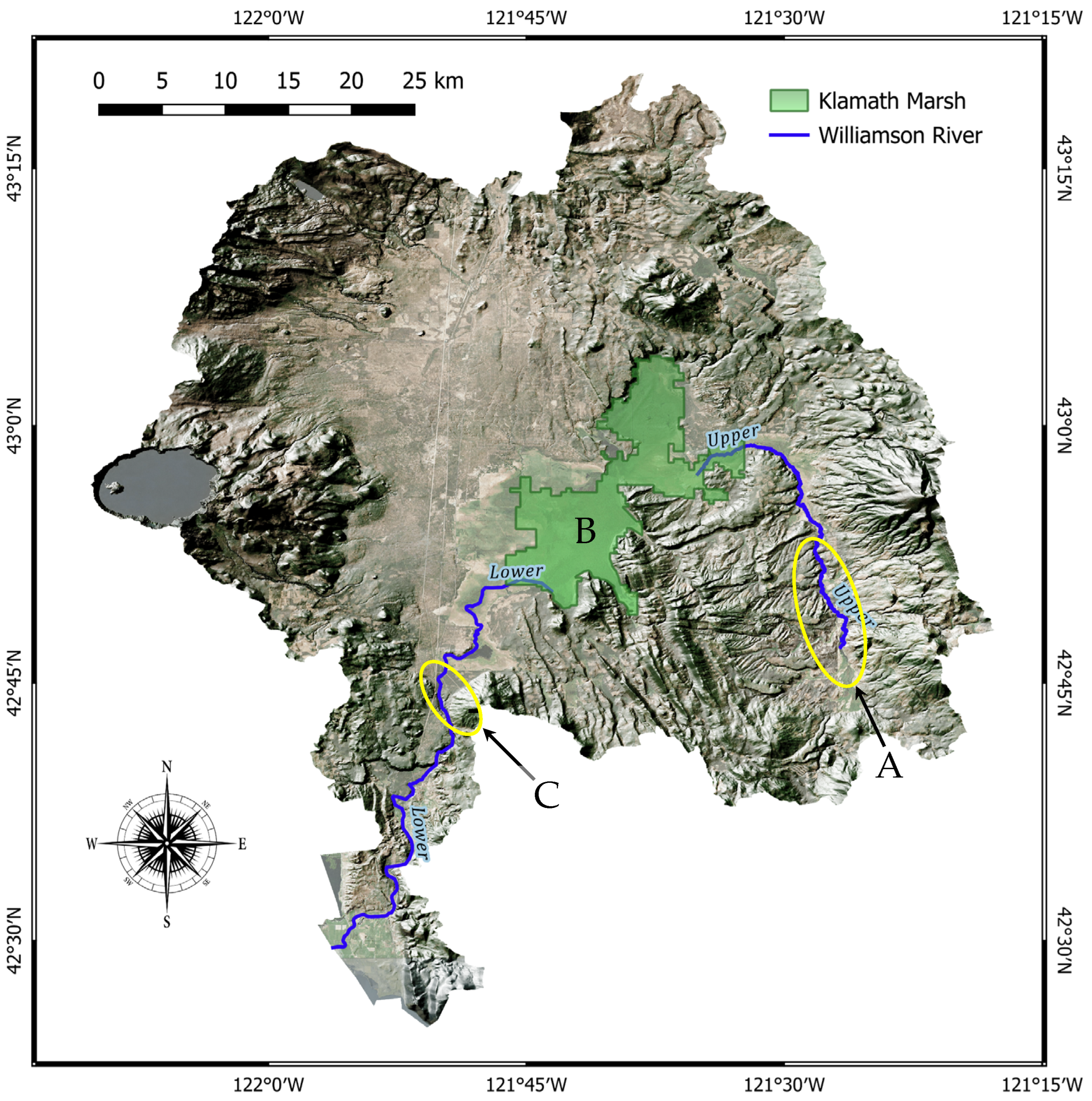
2. Details of the Field Site

2.1. Lithology of the Watershed

The Williamson Basin is approximately 3720 km² (1436 mi²) in size and is located on the eastern edge of the Cascade volcanic range. The northern, eastern, and southern boundaries are enclosed by tertiary volcanics and the fault-block geology of the basin and range province. Mount Mazama is the high point of the basin at 2486 m (8157 ft), which then slopes downward to an elevation of 1245 m (4090 ft) at the Klamath Marsh. A simplified geology of the basin subdivides the lithology into three major geological units: (1) the surficial pumice blanket; (2) intertwined beds of sand, clay, gravel, pyroclastics, and basalt (Yonna formation); and (3) the underlying andesitic/basaltic bedrock, which is the main water-bearing unit [2,4,5,7,8,57]. On the surface, pyroclastic fall pumice, ash, and other volcaniclastics from Mt. Mazama blanket the basin from the Crater Lake down to the Klamath Marsh. Newcomb and Hart [57] labeled this the “Mazama Pumice Plain” and documented its highly porous nature with infiltration rates on the order of 10⁻⁴ m/s (3.28 × 10⁻⁴ ft/s) [7]. Internally, the bedrock aquifer has interbedded vesicular scoriaceous tuff, is highly fractured, and displays columnal jointing. Aquifer pumping tests have a high transmissivity with average values of approximately 15,800 m²/day (170,000 ft²/day) [6].

Historically, the groundwater levels have fluctuated in response to climatic cycles, ranging from years to decades, with the groundwater levels and springs responding to wet and dry periods. Areas with groundwater level changes of 1.5 m (5 ft) have been noted by researchers as common, with fluctuations up to 3.6 m (12 ft) observed in regions closer to the Cascades [9].

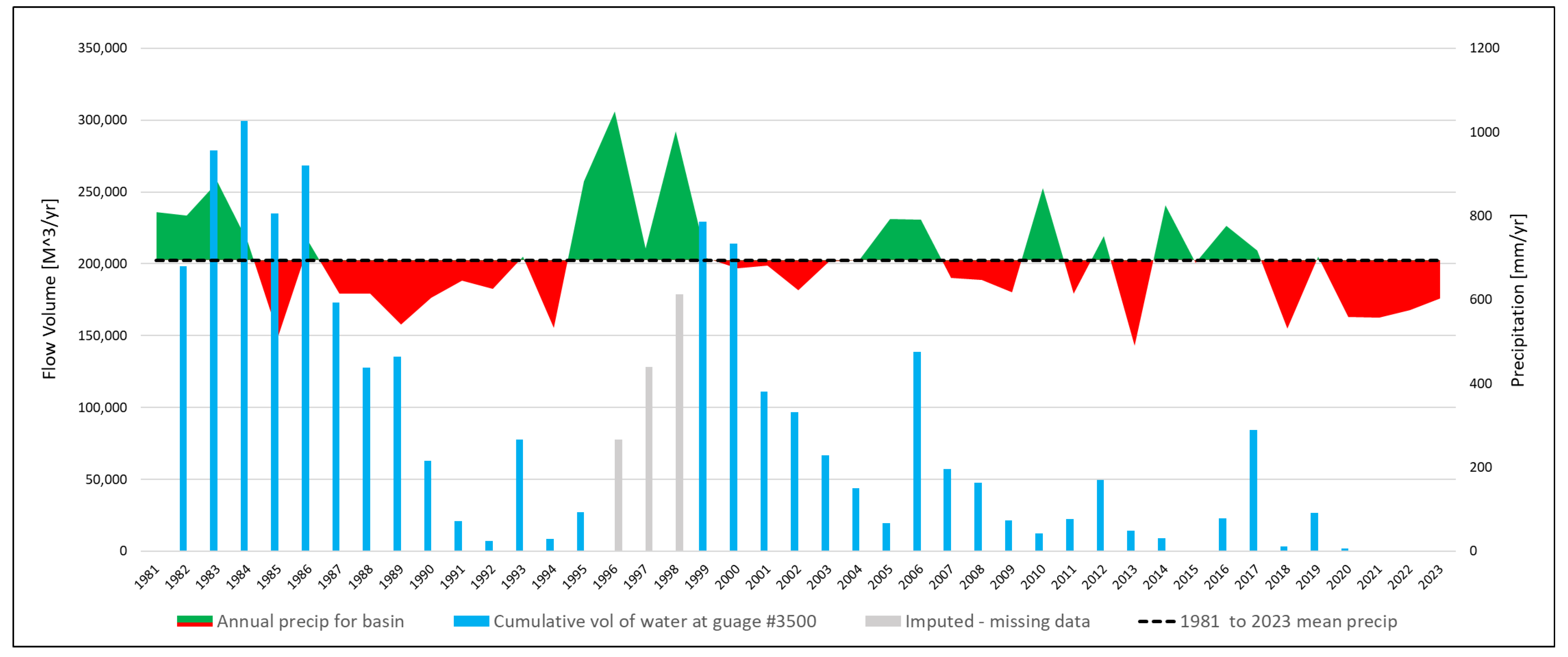
2.2. Basin Precipitation

The Cascade Mountains (including Mount Mazama) receive upward of 150 cm (60 in) of precipitation per year, mostly as snow. The central and eastern portions of the range, which lie in the rain shadow, receive as little as 45 cm (18 in) of precipitation per year [2,5]. Temperatures range from highs of 40° C to lows of −31° C. The revised Köppen–Geiger classification identifies the Williamson Basin as warm, dry summer continental, and the high elevation rim is classified as being dry, sub-arctic [58].

Snowfall and snowmelt recharge the groundwater system through the highly porous desert soils and alluvium along the high elevations of the Cascade Range. Previous research estimates that this spongelike geology can absorb and move upwards of 3.7 × 10⁷ m³ (30,000 acre-ft) of water into the aquifer [4,57]. Because of this, many named and unnamed tributaries start in the high mountains and disappear into the sub-surface, leaving the area absent of typical drainage morphology. Maps show that the Sand, Scott, Miller, and Cottonwood Creek all disappear into the alluvium before reaching confluence with the Williamson River.

Because the Klamath Marsh acts as both a terminus for surface flow and acts as the groundwater-driven headwaters of the Williamson River, rainfall/runoff models of this watershed are typically inaccurate, as streamflow is not directly driven by precipitation. We performed an analysis of the 12-month cumulative precipitation volume to gage the flows and confirmed that a correlation exists between precipitation and flow on a year-to-year basis but is weak (Figure 3). Streamflow generally declines following dry periods and increases during wet periods, although the full impact of the precipitation on the streamflow is delayed by several years. This delay between precipitation and streamflow can be explained by interactions with groundwater storage, which we illustrate later in this paper.

Uncoupled from a conventional rain–runoff relationship, the true headwaters of the Williamson River are at the Klamath Marsh. Isotropic analysis performed by Melady (2002) and Cummings (2007) confirmed distinct differences in the deuterium and oxygen isotope ratios in the surface and groundwater, along with distinguishable concentrations of magnesium, calcium, potassium, and sodium that demonstrate that the streamflow is from groundwater sources [5,7].

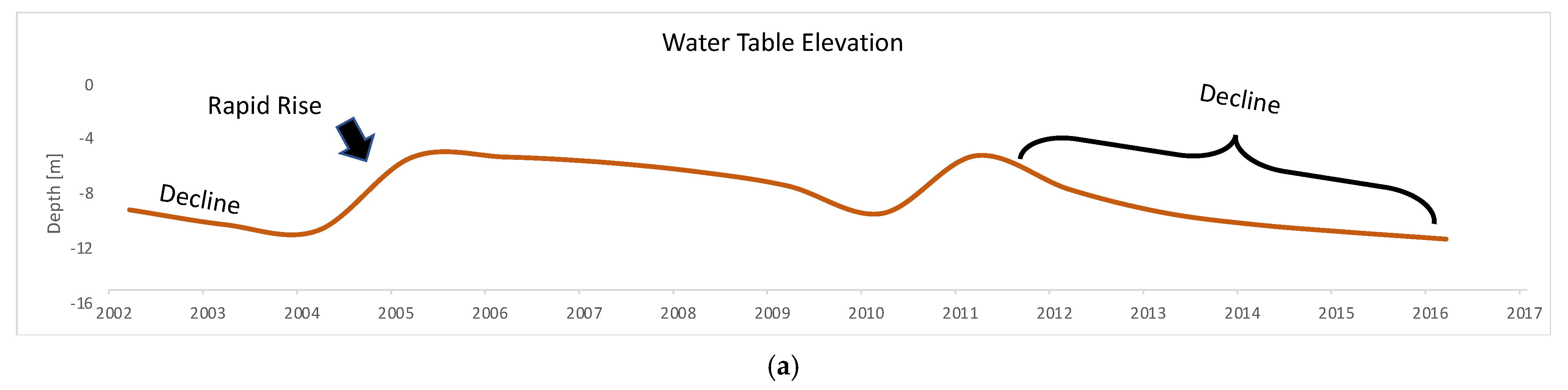
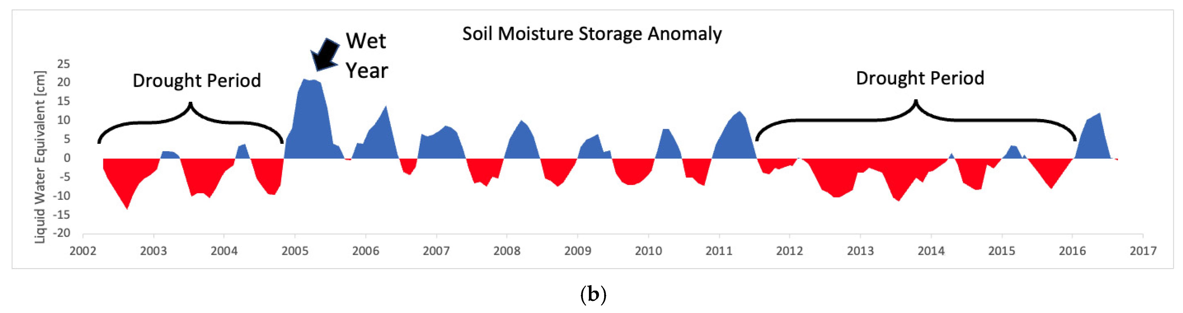
2.3. Drought Impacts in the Basin

Annual precipitation and streamflow data for the basin show two multi-year drought periods since 1981 (Figure 3). The first drought was from 1990 to 1994, culminating in extremely low streamflow. The second drought was longer, beginning in 2020 and continuing to the winter of 2023.

While the first drought was shorter, there were three drier than normal years prior to the 1990–1994 drought, which should be included as they affect groundwater storage. This first drought period culminated in extremely low flows that were temporarily relieved by a wetter than normal winter in 1993. On average, observed flow volumes during this first drought period ranged from between 29 and 75 percent lower than flows in the previous decade. Unfortunately, the gage was deactivated in October 1995 and subsequently reactivated in September 1998. After the gage was reactivated, the water volumes in 2000 and 2001 indicate that the aquifer is capable of being recharged and that the storage capacity of this system is not impaired by such impacts.

The second drought, from 2020 to 2023, was the result of similar low precipitation volumes. Figure 3 shows that yearly precipitation volume has been declining since about 1998, with 2006, 2007, 2011, 2013, 2015, and 2017 being well above average, but most years show a trend toward a declining average. The remaining years since 1998 are below average, with 2014 and post-2018 extremely low. This long-term decline in precipitation, starting in about 2008, has depleted the watershed entirely, with 8 April 2021 being the last date any surface water was measured leaving this watershed.

3. Datasets Used in the Study

3.1. Groundwater Level Monitoring Well Data

Both the USGS and the Oregon Water Resource Department (OWRD) maintain monitoring wells in the basin study area. We used 12 active monitoring wells (4 USGS, 8 OWRD) and 11 inactive wells (all OWRD), with various periods of activity since the 1960s. The depth of our sample wells averages 280 ft, with a range between 75 ft and 670 ft. Of the 15 wells with accessible logs, 13 are in the Klamath volcanic area, a locally confined highly porous aquifer [2]. The remaining two are in the Yonna formation (see Section 2.1). When active, more recent measurements have a resolution of 0.3 cm (0.01 ft), but older measurements are sometimes recorded with a coarser resolution of 3–30 cm (0.1–1.0 ft). Figure 4 shows the monitoring well locations used in this study. Well records prior to 1968 did not include enough data for the GWDM tools due to both the low number of data points and a low data resolution. After removing 2 wells with insufficient data, the dataset included 21 wells with 1312 water level records. We examined the water level data and eliminated four measurements that appeared to be outliers resulting either from recording errors or faulty depth measurements. The final dataset included 1308 measurements that we used in the analysis. The full dataset including well locations and the water level records is available in the HydroShare.org data repository [59] described in the Supplementary Materials section below.

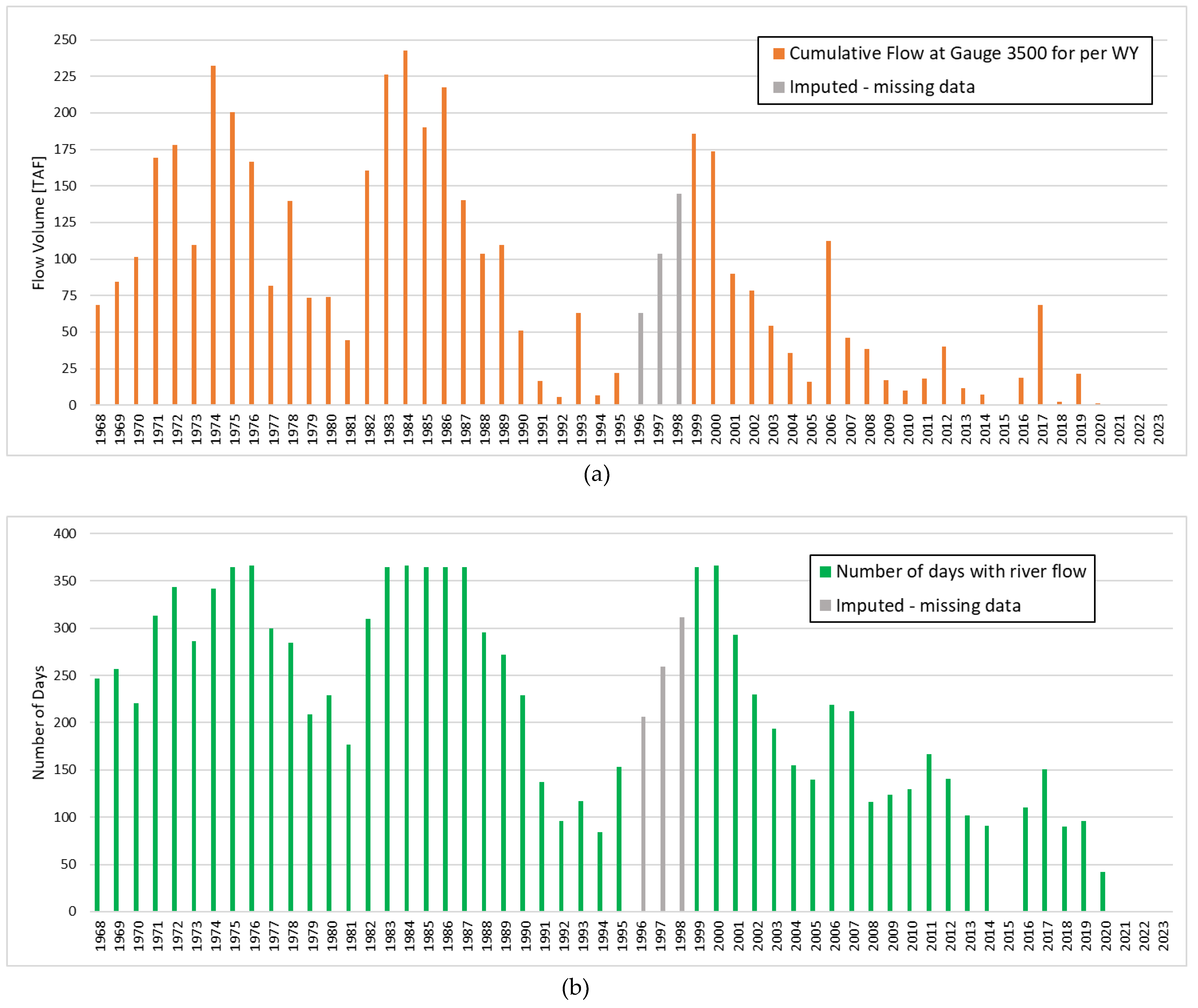
3.2. Streamflow Data

Flow in the Williamson River is measured at the US Geological Survey (USGS) streamflow gage number 11493500 (gage #3500), located at approximately 42.740° N, −121.834° W; it is 0.5 km (0.31 mi) south of the topographic high known as Kirk Reef (Figure 2, area C). Installed in 1954, the gage records discharge on a daily timestep in cubic feet/s (CFS). We used these data to compute cumulative annual flow volumes as thousands of acre-feet (TAF) per year, which is the measurement commonly used by irrigators and water managers in the western United States. One acre-ft is approximately 1233.5 m³, and one acre-ft per day is approximately 0.504 CFS (0.0143 m³/s).

Figure 5 shows the cumulative annual flow per year in TAF (Figure 5a) and the number of days per year of non-zero flow at gage #3500 (Figure 5b). The gage was deactivated on October 1995 and reactivated on September 1998, creating a 3-year gap in the data. For our analysis, we imputed streamflow values for this 3-year gap using linear interpolation to ensure that the missing values are not interpreted as zero flow in our analysis, since actual recorded zero flow values do occur in the record.

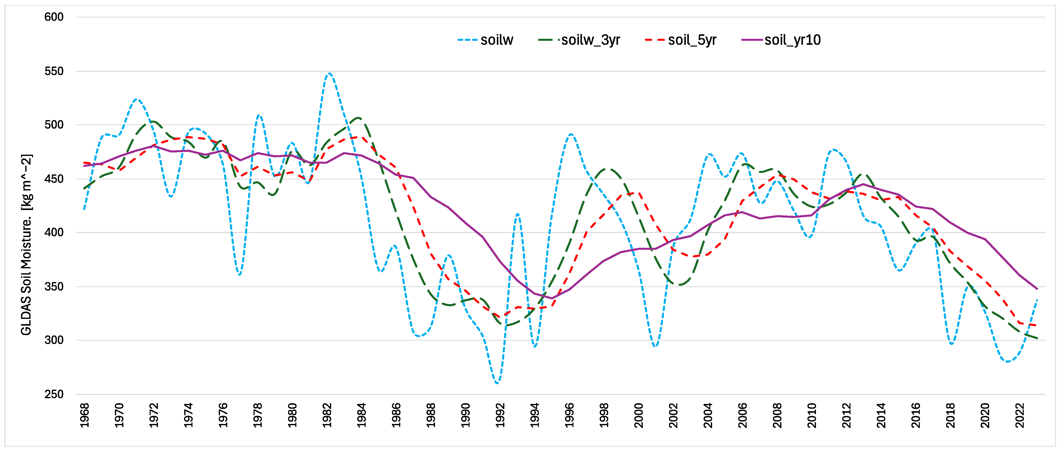
3.3. GLDAS Soil Moisture Data

To impute missing groundwater measurements at a selected well, the GWDM tools use the measured data at the well combined with the soil moisture dataset from the NASA Global Land Data Assimilation System (GLDAS), which is a global gridded dataset [60]. GLDAS consists of three separate land surface models: LSM, Noah, and VIC. We used the monthly averaged results from the Noah model, which has a resolution of 0.25 × 0.25 degrees. We downloaded these data from the Goddard Earth Sciences Data and Information Services Center (GES DISC) website [61].

3.4. Precipitation Data

We used precipitation data from the CHIRPS gridded data product developed by the Climate Hazards Center at UC Santa Barbara in collaboration with the USGS Earth Resources Observation and Science (EROS) Center [62]. The CHIRPS dataset is derived from a variety of NASA and NOAA Earth observation sources and aggregated to a high-resolution global grid (0.05°) covering a period from 1981 to the present. We obtained CHIRPS data for the Williamson Basin, from the NASA SERVER ClimateSERV website [63]. To download the data, we first uploaded a GEOJSON file, which defined the boundaries of the basin. The website then provided a time series of daily rainfall data consisting of the daily average precipitation of the CHIRPS grid cells in the interior of the basin. We elected to use the CHIRPS dataset over data from individual rain/snow gages in the basin because our objective was to perform a groundwater storage analysis in a manner that aggregates both in situ data and Earth observations of the entire basin. The CHIRPS data represent a basin-scale, gridded dataset that is consistent with our basin-scale groundwater analysis.

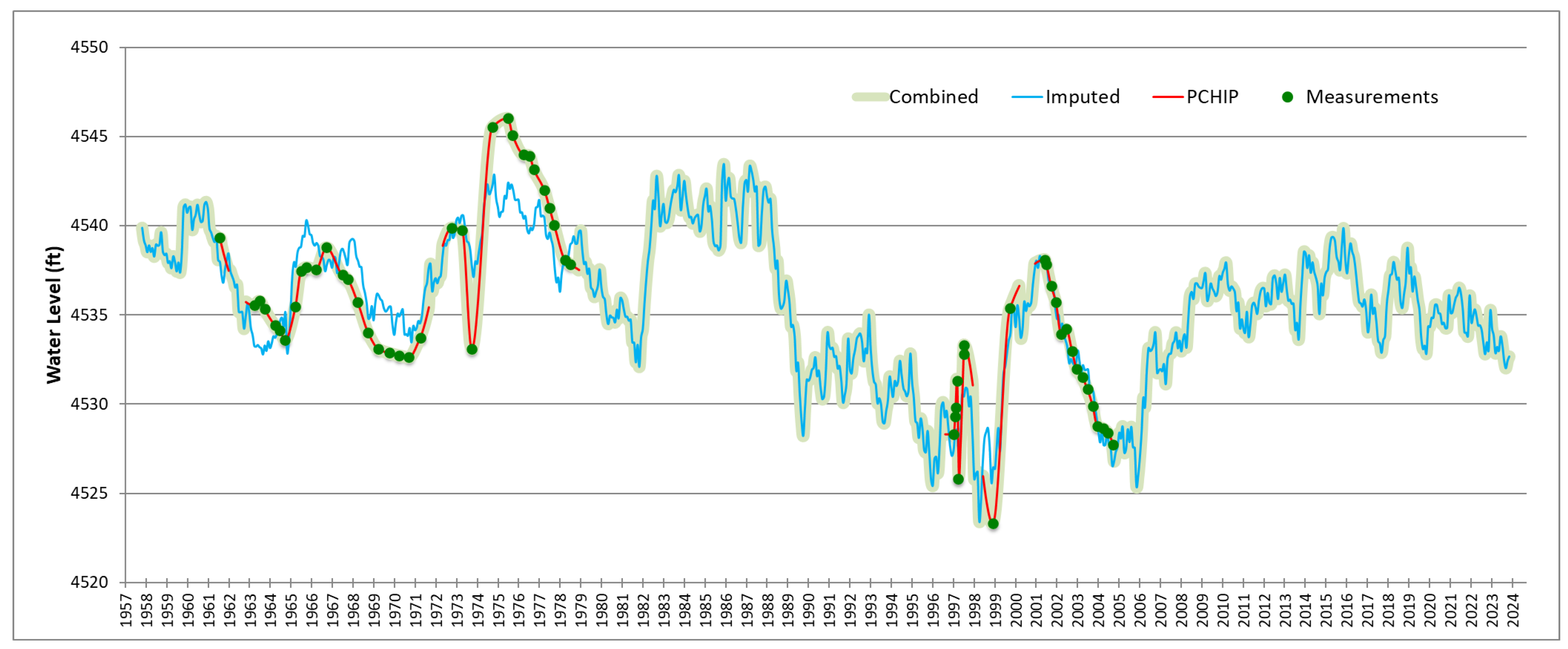
4. Interpolated Groundwater Level Data Using GWDM

We generated an estimate of the historical groundwater storage changes in the Williamson Basin using the tools available within the GWDM platform [49]. GWDM uses a combination of in situ water level data and Earth observations in a multi-step process to estimate aquifer storage changes [48,50,51]. In the first step, the user imports well locations and historical water levels that define a water level time series for each well. However, it is common to have significant gaps in historical water level records at a well, ranging from several months to several years. Since computing the aquifer storage change requires a relatively complete water level record at each well, GWDM uses a machine learning algorithm to impute missing data for each well over the study period. The theoretical basis for this algorithm is that groundwater levels are highly correlated with drought indicators such as soil moisture; see Figure 6. During a drought, there is less groundwater recharge, and groundwater is pumped at a higher rate to meet agricultural, municipal, and industrial demands. During wet periods, there is a higher rate of recharge and less pumping. As a result, groundwater levels drop during drought periods and rise during wet periods. The machine learning algorithm learns these relationships, often non-linear, and uses them to impute missing values. The complete well records are then sampled at regular intervals and spatially interpolated to a set of time-varying rasters that are used to compute groundwater storage change vs. time. The entire process is described in more detail in [49,50,51,64]. GWDM uses an Extreme Learning Machine (ELM) model, which performs a linear analytical fit on all the available data; thus, there is no testing or training split. The model features include GLDAS results such as soil moisture, the flux and lags of soil moisture anomalies, and smoothed soil moisture averages over a 10-year period. As the GWMD model, features, and accuracy assessment methods are well defined in the literature and are published as an open-source tool, we do not repeat them here [49,50,51,64].

After the initial imputation, GWDM refines the imputed data using correlations among the existing well data and imputed results. This reduces uncertainty and provides a check on the imputed data. The GWDM tools include a set of Python scripts for cleaning and formatting data and for performing the imputation and volumetric analysis [49]. The wells, water levels time series, interpolated water level rasters, and groundwater storage time series can be uploaded and visualized in a web application [48,65].

To apply this process to the Williamson Basin, we used the well locations and associated water level measurements and created a water level time series for each well. Next, we used piecewise cubic hermite interpolating polynomial (PCHIP) interpolation to impute data for all gaps in the monthly water level records for each well. We retained these imputed values for gaps less than two years. We then deleted the PCHIP-interpolated values for gaps greater than or equal to two years while retaining 180 days of PCHIP-imputed data at the beginning and end of each of these gaps. At the end of this step, we have imputed the small gaps in the water level time series at each well, but the large gaps remain, with imputed data at the beginning and the end within 180 days of measured values.

Next, we used the GWDM tools to build a separate machine learning model for each well using the Extreme Learning Machine (ELM) algorithm, which directly solves the linear optimization problem without iterative training [48]. The model features for each well are the monthly GLDAS soil moisture anomalies corresponding to the centroid of the basin and the three-, five-, and ten-year moving average of the soil moisture anomaly for the period from 1968 to 2023. The moving averages capture longer-term trends in the data. Additional model features are the year and one-hot encoded month indices to capture seasonality and non-stationary trends in the data. We fit a separate ELM model for each well using the observed water levels as the dependent variable.

We used the ELM models to impute missing data to generate a complete water level record for each well from 1968 to 2023. Finally, we combined the measured, PCHIP, and EML datasets into a single water level dataset where the priority was the measured data, then the PCHIP data (short gaps), and then the ELM-imputed data for the longer gaps. In other words, for all months where there was either a measurement or PCHIP-interpolated value, we used that value. If no measurement or PCHIP value was available, we used the EML-imputed data value.

We sampled the time series at each well on yearly intervals from 1968 to 2023. We spatially interpolated these data to a 150 × 150 grid, which we then clipped to the basin boundaries, resulting in a yearly groundwater elevation map for the basin over the study period. We calculated the volume between each subsequent pair of groundwater elevation rasters and then multiplied the value, which represents the water level change, by a representative unconfined storage coefficient for the basin (0.1) to generate annual groundwater volume changes; then, we integrated these values to generate a groundwater storage curve for the basin.

5. Results

5.1. Correlation Between Precipitation and Flow Data

Before exploring the relationship between groundwater and streamflow in the basin, we first examined the relationship between precipitation and streamflow. We interpolated the annual cumulative data to estimate values at the start of each month. Cumulative annual flow data for three years, 1996–1998, were not available because the gage was deactivated during this period, so data in this period are all linearly interpolated from the values on each side of the gap. We normalized both datasets using standard score (z-score) normalization and found that a weak correlation exists between precipitation and flow on a year-to-year basis (Figure 7a). The Pearson correlation coefficient (r) of annual cumulative rainfall to annual cumulative flow by year is r(n = 41) = 0.29, p = 0.06, which shows that the two series are only slightly correlated. Nevertheless, streamflow generally declines following dry periods and increases during wet periods, but the full impact of the precipitation on the streamflow is delayed by several years.

To better characterize the correlation between cumulative annual precipitation, we computed the Pearson correlation coefficient using monthly lags from −60 to +60 lags (±5 years) between the two series. We found that the highest correlation occurs at a lag of −32 months, with r = 0.525, p < 0.001 (Figure 8). The computed p-value is essentially zero but is based on the interpolated monthly values, so it is not representative of the data. Our analysis showed that there is not a sharp peak in the correlation values, but a relatively smooth transition. This indicates that the lag that produces the highest correlation probably changed over the 43-year study period. We would expect a longer lag at low groundwater levels and a shorter lag at high groundwater levels. Figure 7b shows cumulative annual precipitation data plotted with cumulative annual flow data lagged by 32 months. In general, these two datasets are visually correlated. The no-data period, from 1996 to 1998, is not as visually correlated, as the interpolated data do not follow precipitation.

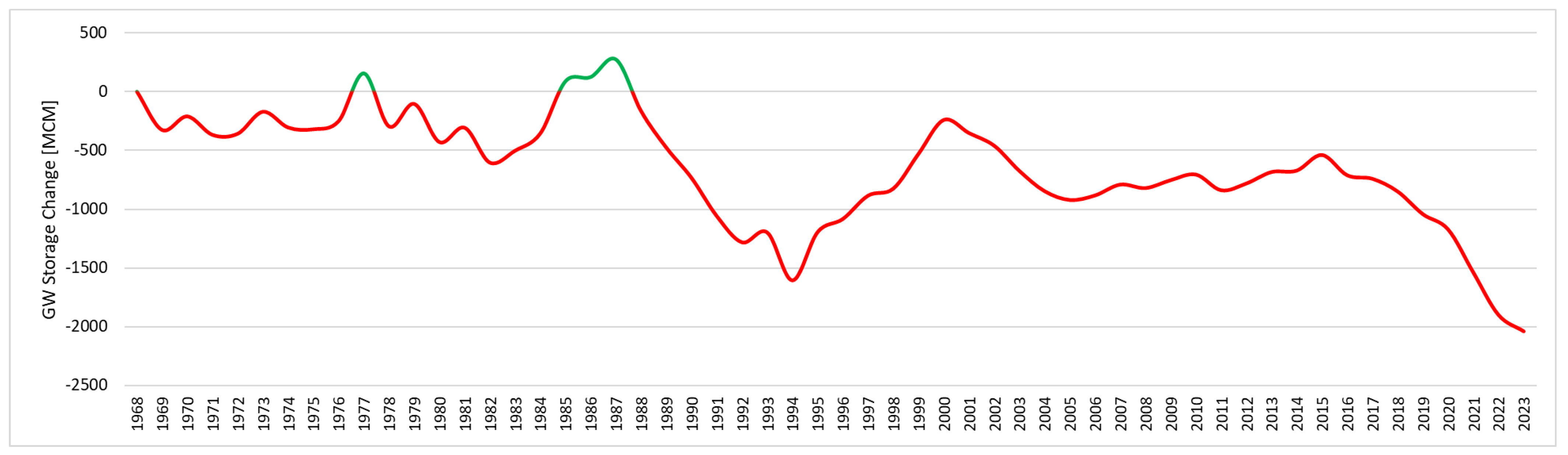
5.2. Groundwater Storage Change

To better understand the correlation between groundwater and streamflow, we derived the groundwater storage change using the GWDM tools. The monthly GLDAS soil moisture (soilw) dataset for the GLDAS grid cell containing the centroid of the Williamson Basin and the 3, 5, and 10 yr moving averages of the soil moisture are shown in Figure 9.

Using PCHIP interpolation and the ELM models for each well, we generated a complete set of water levels for each well. Figure 10 shows an example set of measured and imputed water level time series data for well KLAM0000496 in the Williamson Basin. The “combined” trace in the figure represents the data we used for this study.

We used the generated water level time series, for each well, to generate a groundwater storage curve for the basin as shown in Figure 11. The volumetric storage change values are relative to the starting value of zero in 1968. Figure 11 shows that groundwater storage was relatively constant from 1968 through 1987 and then dropped significantly for 7 years before partially rebounding from 1994 to 2000. This rebound was followed by a decline from 2000 to 2005 and then a steeper decline starting in 2015 that has continued through the end of 2023. These data show that the basin has lost approximately 2000 million m³ (1600 TAF) over the 55-year study period. Soil moisture shows a similar decline (Figure 9), indicating both processes are driven by climatic conditions.

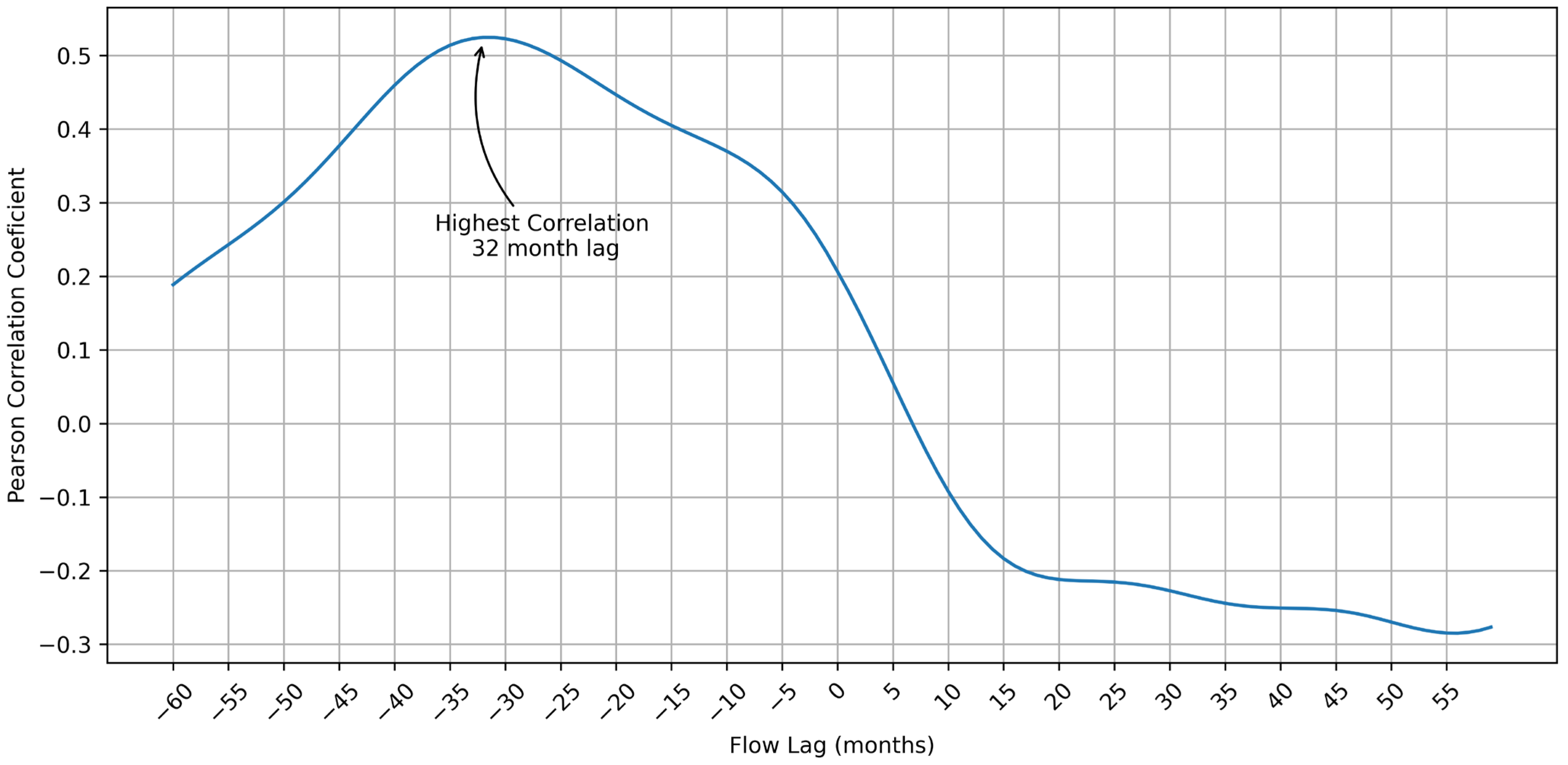
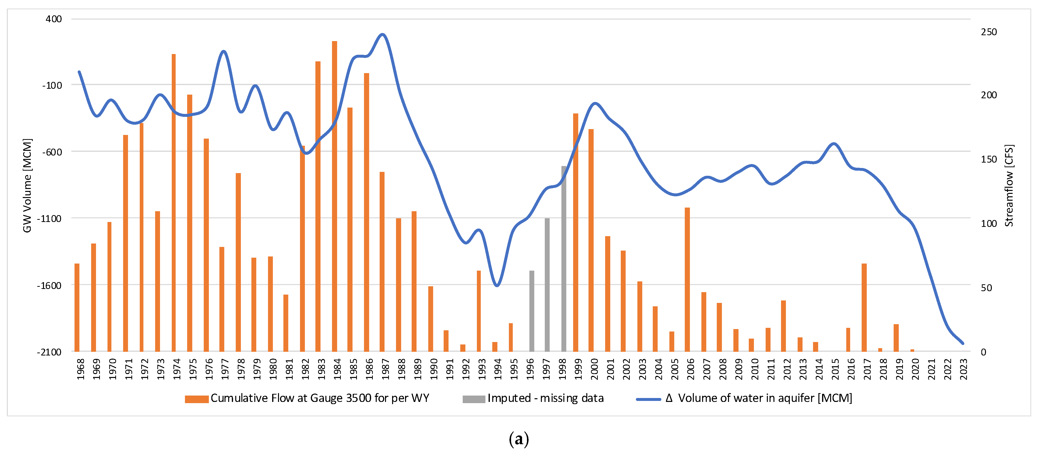
5.3. Groundwater–Streamflow Correlation

Figure 12a compares the groundwater storage curve to the cumulative streamflow data at gage 3500. Visually, there is a strong correlation between the decline in groundwater storage and declining streamflow from 1985 to 1995, followed by a rebound in both 1985 and 2000. After the rebound, both streamflow and storage declined through 2005, which was followed by a steeper decline in groundwater storage starting in 2015. This decline in groundwater storage is followed by a complete cessation of streamflow in 2021. The Pearson correlation coefficient between the groundwater storage and streamflow is r(n = 54) = 0.64, p < 0.01, relatively well correlated.

Figure 12b shows the groundwater storage and the days per year with non-zero streamflow. The same overall behavior is observed, but groundwater storage is even more strongly correlated with flow days, resulting in a Pearson correlation coefficient of r(n = 54) = 0.79, p < 0.01.

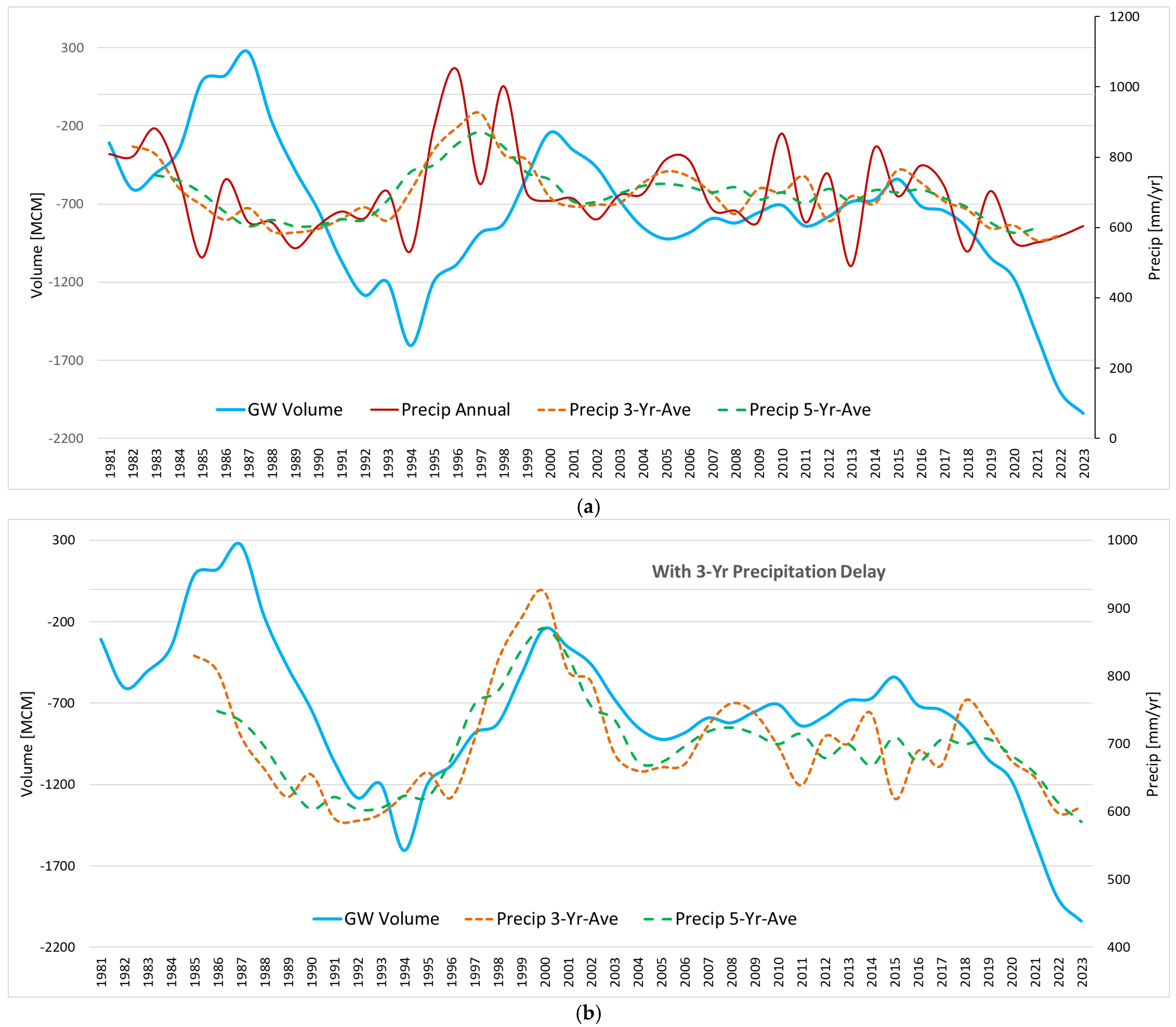
5.4. Groundwater Storage Change and Rainfall Correlation

Finally, we examined the relationship between groundwater storage change and precipitation. We started the comparison in 1981 as opposed to 1968, as the CHIRPS data were not available prior to 1981. Figure 13a shows groundwater storage change versus cumulative annual precipitation along with the 3- and 5-year moving average of the cumulative precipitation. The figure shows that long-term changes in groundwater storage mirror fluctuations in precipitation, particularly the 3 and 5 yr moving averages, but the peaks and valleys are offset. We evaluated different lags and found that, if we lag groundwater storage by 3 years, we achieved a high degree of correlation with both the 3 and 5 yr precipitation curves as shown in Figure 13b. This matches the lag we found between precipitation and streamflow in Section 5.1.

The Pearson correlation coefficient for lagged groundwater storage and 3 yr and 5 yr moving average precipitation are r(n = 37) = 0.60, p < 0.01, and r(n = 36) = 0.64, p < 0.01, respectively. This indicates that it takes approximately 3 years for precipitation to fully percolate through the vadose zones and flow into the basin to effectively recharge the groundwater in the basin aquifers. Even though the precipitation in the basin started to rebound in 2021, as shown by the solid red line in Figure 13a, the groundwater still has not started to rebound, as it is most closely correlated with the 3 and 5 yr moving average of precipitation with a 3 yr delay. Once groundwater in the basin has rebounded to a high enough level to feed the seeps and springs at the head of the Williamson River, we expect the flow to resume.

6. Discussion

Due to the geology of the Williamson Basin, river flow is uncoupled from a conventional rain–runoff relationship with little short-term relationship between precipitation and flow. Studies have shown that the headwaters of the Williamson River are at the Klamath Marsh and are related to groundwater rather than the tributaries that feed the marsh. Isotopic data have shown distinct differences in deuterium and oxygen isotope ratios in the surface and groundwater, along with distinguishable concentrations of magnesium, calcium, potassium, and sodium, supporting this conclusion [1,6]. These studies, combined with the lag between precipitation and streamflow demonstrated in Section 5.1, indicate that flow in the Williamson River is governed by groundwater. Lagged correlation with precipitation, streamflow, and groundwater storage indicates that precipitation in this basin recharges groundwater over about a 3-year time period. However, while precipitation and recharge are coupled and demonstrate a correlation in time, the correlation between groundwater and streamflow may be more complex. A simple analogy would be a bathtub; enough water must fill the tub before it can overflow, and in a similar manner, we propose that groundwater underneath the National Wildlife Refuge needs to reach a certain volume before it can discharge through the various springs and seeps. Groundwater levels below this level result in low-flow or no-flow conditions from this basin.

The general relationship between the groundwater storage volume and Williamson River flow has traditionally been known to hydrogeologists and those with local knowledge, but a detailed characterization of basin processes with a method to estimate long-term changes in groundwater storage was previously unavailable. This is because examining water levels at individual groundwater monitoring well locations does not capture the full behavior of the groundwater–surface water interaction, as individual wells may not provide insight into aquifer storage due to incomplete records and local behavior at a well.

The tools we used in this study provide methods to address these issues. The imputation of groundwater level data for each well using correlations between well data and Earth observations addresses sparse data at the wells. The spatial interpolation and mapping algorithm uses these individual well data and computes a time series of aquifer level maps that can be integrated to provide aquifer volume changes. Computing these storage changes and integrating them over time provides the basis for the analysis we presented in this paper. These tools provide insights that allow us to better characterize the relationship between precipitation, groundwater, and streamflow in the Klamath Basin and the effects of climate change on this area. This is a novel approach, as the majority of groundwater analysis tools do not compute groundwater changes on a yearly timestep [52]. Our tools allow us to use the available, but gap-filled, groundwater level data in the Klamath Basin along with precipitation records to characterize the precipitation–groundwater–streamflow interactions in a manner that was previously not possible. This hydrologic system description and understanding allows managers and others to evaluate and gage the impact of droughts and anthropogenic actions on the Klamath Basin.

Our analysis confirms that the overall volume of water within the aquifer is strongly correlated with streamflow leaving the watershed. As illustrated by the drought in the 1990s and the current drought, once the groundwater storage drops approximately 1800 MCM (1500 TAF) below the 1968 baseline, streamflow in the basin ceases completely. Due to the multi-year delay between precipitation and groundwater storage, even though precipitation has rebounded in the last three years, the groundwater has not yet responded, as the groundwater storage has not reached the critical level. Our analysis suggests that it should rebound soon. If precipitation continues at recent rates, we should expect streamflow to return in the next 3–5 years.

More concerning is the trend seen in the aquifer volume since 2001. Combined with the continuous decline in streamflow shown in Figure 12a, this indicates an overall drop in the total volume of groundwater within the basin. This trend is possibly anthropogenic. It coincides with actions taken by various federal agencies as part of a biological consultation. As a result of the National Marine Fisheries Service (NMFS)’s 2002 biological opinion on the endangered Chinook Salomon (Oncorhynchus tshawytscha), the Bureau of Reclamation reduced demand and stored extra water for the endangered species. The goal was to create a “water bank and water supply to provide flows to the Klamath River below Iron Gate Dam to improve coho salmon habitat” [67]. Designed to save water for habitat flows, up to 100 TAF of water was to be conserved in Upper Klamath Lake. Conservation was achieved through land idling, increased storage of surface water, and the encouragement of groundwater usage to supplement/replace diverted live flow or deliveries of project water [67,68]. These policies may have contributed to the depletion of groundwater storage.

Supporting this theory is the sharp drop in groundwater in 2020 and the resulting no-flow conditions at gage #3500. Using the CHIRPS data, we can roughly estimate that 3468 MCM of water (2811 TAF) entered this watershed between 2020 and 2023, with only 1.6 MCM (1.3 TAF) of outflow measured during the same 4-year period. This coincides with a severe drought and an increase in surface water restrictions, leading to increased groundwater consumption. Further research is needed to separate out anthropogenic pumping impacts on this watershed.

On a positive note, the groundwater storage increase from 1994 to 2000 illustrates that, with sufficient precipitation, the aquifer storage is capable of rebounding substantially. This understanding can and will assist in management decisions. This knowledge allows managers to properly manage a high water supply forecast from an above-normal snowpack, as water managers can adjust their forecast with awareness about aquifer recharge and storage. Biologists and natural resource managers, aware of the timeframe and water availability, can adjust management and conservation plans for aquatic species [6,66].

As with all imputation methodologies, the resulting data inherently possess a degree of error and uncertainty. The GWDM framework generates an initial model and imputes results for each individual well, iteratively refining these outputs by incorporating data from all wells within the aquifer system. This iterative process minimizes uncertainty and significantly reduces large deviations. Subsequently, spatial interpolation is applied to the groundwater elevation data at each temporal step, meaning that each well contributes only to the localized portion of the interpolated surface. Comparative studies of published GWDM results with established United States Geological Survey (USGS) models have demonstrated strong concordance between methodologies [49,50,51,64]. While the uncertainty associated with the imputed data in this study remains unquantified, the primary objective is to assess long-term trends and their correlation with processes such as precipitation and streamflow. Despite the inherent uncertainties, the long-term trends have reduced variability. Though unquantified uncertainty exists, our analysis of groundwater storage and how it is related to precipitation and stream flow is valid.

7. Conclusions

The primary objective of this research was to use a groundwater storage analysis tool to characterize the time history of groundwater storage in the Williamson Basin by supplementing sparse in situ data with Earth observations. The resulting groundwater storage data allowed us to gain new insights into the complex relationship between precipitation, groundwater, and streamflow in the basin. Using the data from this analysis, we have demonstrated that both streamflow quantities and the number of days per year with streamflow are highly correlated with the groundwater storage levels, and once the groundwater storage drops below 1800 MCM (1500 TAF) relative to the 1968 baseline, the streamflow in the basin completely ceases. We computed that there is a 3 yr lag between the 3 and 5 yr moving average precipitation in the basin and groundwater storage once this threshold is reached. This means that, even though precipitation has started to rebound in the basin, it will take several more years, more than the 3-year lag, of elevated precipitation before the streams begin to flow again. This is because the time required includes both the 3-year lag and the time required to recharge the aquifer to the critical level. The high level of correlation we found between precipitation, groundwater storage, and streamflow validates the use of the new groundwater storage tools that we applied. This approach represents a new technique that water managers can use in groundwater-dependent basins to better understand and more effectively manage precious water resources.

The methods and tools demonstrated in this study, particularly the GWDM tools, the associated framework, and the use of globally (and freely) available GLDAS data, have significant potential for application in other basins and locations. This approach is especially valuable for regions with sparse measured groundwater data, as it enables the integration of Earth observations to address gaps in data and refine groundwater storage estimations. By using publicly accessible resources and computational techniques, the framework can be adapted to analyze precipitation–groundwater–streamflow interactions in diverse hydrologic systems worldwide. Its ability to characterize and incorporate long-term trends and manage uncertainties makes it an effective tool for water managers and researchers dealing with groundwater-dependent basins, offering insights to improve resource management even in data-limited regions.

References

1. Ochoa, C.G.; Jarvis, W.T.; Hall, J. A Hydrogeologic Framework for Understanding Surface Water and Groundwater Interactions in a Watershed System in the Willamette Basin in Western Oregon, USA. Geosciences 2022, 12, 109. [Google Scholar] [CrossRef]
2. Conaway, J.S. Hydrogeology and Paleohydrology in the Williamson River Basin, Klamath County Oregon. Master’s Thesis, Portland State University, Portland, OR, USA, 2000. [Google Scholar]
3. Mayer, T.; Wurster, F.; Craver, D. Klamath Marsh Hydrology and Water Rights; USFWS: Washington, DC, USA, 2007; p. 22. [Google Scholar]
4. Leonard, A.R.; Harris, A.B. Ground Water in Selected Areas in the Klamath Basin, Oregon; Oregon Water Science Center: Portland, OR, USA, 1974; p. 104. [Google Scholar]
5. Melady, J. Hydrogeologic Investigation of the Klamath Marsh, Klamath County, Oregon. Master’s Thesis, Portland State University, Portland, OR, USA, 2002. [Google Scholar]
6. Gannett, M.W.; Lite, K.E., Jr.; Marche, J.L.L.; Fisher, B.J.; Polette, D.J. Ground-Water Hydrology of the Upper Klamath Basin, Oregon and California; Geological Survey (U.S.): Reston, VA, USA, 2007. [Google Scholar]
7. Cummings, M.L. Hydrogeology of the Williamson River Basin, Upper Klamath Basin, Klamath County, Oregon. Master’s Thesis, Portland State University, Portland, OR, USA, 2007; p. 70. [Google Scholar]
8. Stannard, D.I.; Gannett, M.W.; Polette, D.J.; Cameron, J.M.; Waibel, M.S.; Spears, J.M. Evapotranspiration from Wetland and Open-Water Sites at Upper Klamath Lake, Oregon, 2008–2010; USGS: Reston, VA, USA, 2013; p. 66. [Google Scholar]
9. Gannett, M.W.; Wagner, B.J.; Lite, K.E., Jr. Groundwater Simulation and Management Models for the Upper Klamath Basin, Oregon and California; U.S. Geological Survey: Reston, VA, USA, 2012. [Google Scholar]
10. Risley, J.C. Using the Precipitation-Runoff Modeling System to Predict Seasonal Water Availability in the Upper Klamath River Basin, Oregon and California; U.S. Geological Survey: Reston, VA, USA, 2019. [Google Scholar]
11. Markstrom, S.L.; Regan, R.S.; Hay, L.E.; Viger, R.J.; Webb, R.M.; Payn, R.A.; LaFontaine, J.H. PRMS-IV, the Precipitation-Runoff Modeling System, Version 4; U.S. Geological Survey: Reston, VA, USA, 2015. [Google Scholar]
12. Chang, H.; Jones, J. Climate Change and Freshwater Resources in Oregon. In Oregon Climate Assessment Report; Oregon Climate Change Research Institute: Portland, OR, USA, 2010. [Google Scholar]
13. Carroll, R.W.H.; Niswonger, R.G.; Ulrich, C.; Varadharajan, C.; Siirila-Woodburn, E.R.; Williams, K.H. Declining Groundwater Storage Expected to Amplify Mountain Streamflow Reductions in a Warmer World. Nat. Water 2024, 2, 419–433. [Google Scholar] [CrossRef]
14. Mayer, T.D.; Naman, S.W. Streamflow Response to Climate as Influenced by Geology and Elevation1. JAWRA J. Am. Water Resour. Assoc. 2011, 47, 724–738. [Google Scholar] [CrossRef]
15. Hess, G.W.; Stonewall, A.J. Comparison of Historical Streamflows to 2013 Streamflows in the Williamson, Sprague, and Wood Rivers, Upper Klamath Lake Basin, Oregon; U.S. Geological Survey: Reston, VA, USA, 2014. [Google Scholar]
16. Tague, C.; Grant, G.; Farrell, M.; Choate, J.; Jefferson, A. Deep Groundwater Mediates Streamflow Response to Climate Warming in the Oregon Cascades. Clim. Change 2008, 86, 189–210. [Google Scholar] [CrossRef]
17. Brutsaert, W. Long-Term Groundwater Storage Trends Estimated from Streamflow Records: Climatic Perspective. Water Resour. Res. 2008, 44. [Google Scholar] [CrossRef]
18. Dudley, R.W.; Hodgkins, G.A. Historical Groundwater Trends in Northern New England and Relations with Streamflow and Climatic Variables. JAWRA J. Am. Water Resour. Assoc. 2013, 49, 1198–1212. [Google Scholar] [CrossRef]
19. Huntington, J.L.; Niswonger, R.G. Role of Surface-Water and Groundwater Interactions on Projected Summertime Streamflow in Snow Dominated Regions: An Integrated Modeling Approach. Water Resour. Res. 2012, 48, W11524. [Google Scholar] [CrossRef]
20. Ayers, J.R.; Villarini, G.; Schilling, K.; Jones, C.; Brookfield, A.; Zipper, S.C.; Farmer, W.H. The Role of Climate in Monthly Baseflow Changes across the Continental United States. J. Hydrol. Eng. 2022, 27, 04022006. [Google Scholar] [CrossRef]
21. Arnold, J.G.; Allen, P.M. Automated Methods for Estimating Baseflow and Ground Water Recharge from Streamflow Records. JAWRA J. Am. Water Resour. Assoc. 1999, 35, 411–424. [Google Scholar] [CrossRef]
22. Winter, T.C. Ground Water and Surface Water: A Single Resource; Diane Publishing: Collingdale, PA, USA, 2000. [Google Scholar]
23. The NCAR WRF-Hydro® Modeling System Technical Description — WRF-Hydro Modeling System 5.4.0 Documentation. Available online: https://wrf-hydro.readthedocs.io/en/latest/ (accessed on 4 June 2025).
24. NOAA. The National Water Model. Available online: https://water.noaa.gov/about/nwm (accessed on 8 July 2024).
25. Zealand, C.M.; Burn, D.H.; Simonovic, S.P. Short Term Streamflow Forecasting Using Artificial Neural Networks. J. Hydrol. 1999, 214, 32–48. [Google Scholar] [CrossRef]
26. Day, G.N. Extended Streamflow Forecasting Using NWSRFS. J. Water Resour. Plan. Manag. 1985, 111, 157–170. [Google Scholar] [CrossRef]
27. Boyle, D.P.; Gupta, H.V.; Sorooshian, S.; Koren, V.; Zhang, Z.; Smith, M. Toward Improved Streamflow Forecasts: Value of Semidistributed Modeling. Water Resour. Res. 2001, 37, 2749–2759. [Google Scholar] [CrossRef]
28. Snow, A.D.; Christensen, S.D.; Swain, N.R.; Nelson, E.J.; Ames, D.P.; Jones, N.L.; Ding, D.; Noman, N.S.; David, C.H.; Pappenberger, F.; et al. A High-Resolution National-Scale Hydrologic Forecast System from a Global Ensemble Land Surface Model. JAWRA J. Am. Water Resour. Assoc. 2016, 52, 950–964. [Google Scholar] [CrossRef] [PubMed]
29. Hapuarachchi, H.A.P.; Wang, Q.J.; Pagano, T.C. A Review of Advances in Flash Flood Forecasting. Hydrol. Process. 2011, 25, 2771–2784. [Google Scholar] [CrossRef]
30. Markstrom, S.L.; Niswonger, R.G.; Regan, R.S.; Prudic, D.E.; Barlow, P.M. GSFLOW—Coupled Ground-Water and Surface-Water Flow Model Based on the Integration of the Precipitation-Runoff Modeling System (PRMS) and the Modular Ground-Water Flow Model (MODFLOW-2005). Available online: https://pubs.usgs.gov/tm/tm6d1/ (accessed on 8 July 2024).
31. Hunt, R.J.; Walker, J.F.; Selbig, W.R.; Westenbroek, S.M.; Regan, R.S. Simulation of Climate-Change Effects on Streamflow, Lake Water Budgets, and Stream Temperature Using GSFLOW and SNTEMP, Trout Lake Watershed, Wisconsin; U.S. Geological Survey: Reston, VA, USA, 2013. [Google Scholar]
32. Ntona, M.M.; Busico, G.; Mastrocicco, M.; Kazakis, N. Modeling Groundwater and Surface Water Interaction: An Overview of Current Status and Future Challenges. Sci. Total Environ. 2022, 846, 157355. [Google Scholar] [CrossRef]
33. Hughes, J.D.; Petrone, K.C.; Silberstein, R.P. Drought, Groundwater Storage and Stream Flow Decline in Southwestern Australia. Geophys. Res. Lett. 2012, 39. [Google Scholar] [CrossRef]
34. Zipper, S.; Brookfield, A.; Ajami, H.; Ayers, J.R.; Beightel, C.; Fienen, M.N.; Gleeson, T.; Hammond, J.; Hill, M.; Kendall, A.D.; et al. Streamflow Depletion Caused by Groundwater Pumping: Fundamental Research Priorities for Management-Relevant Science. Water Resour. Res. 2024, 60, e2023WR035727. [Google Scholar] [CrossRef]
35. Rodell, M.; Famiglietti, J.S. The Potential for Satellite-Based Monitoring of Groundwater Storage Changes Using GRACE: The High Plains Aquifer, Central US. J. Hydrol. 2002, 263, 245–256. [Google Scholar] [CrossRef]
36. NASA. JPL Monthly Mass Grids—Global Mascons (JPL RL06.1_v03) | Get Data. Available online: https://grace.jpl.nasa.gov/data/get-data/jpl_global_mascons (accessed on 9 January 2024).
37. NASA. Studying the Earth’s Gravity from Space: The Gravity Recovery and Climate Experiment (GRACE); NASA Facts—FS-2002-1-029-GSFC; NASA: Washington, DC, USA, 2002. [Google Scholar]
38. McStraw, T.C.; Pulla, S.T.; Jones, N.L.; Williams, G.P.; David, C.H.; Nelson, J.E.; Ames, D.P. An Open-Source Web Application for Regional Analysis of GRACE Groundwater Data and Engaging Stakeholders in Groundwater Management. JAWRA J. Am. Water Resour. Assoc. 2022, 58, 1002–1016. [Google Scholar] [CrossRef]
39. Scanlon, B.R.; Faunt, C.C.; Longuevergne, L.; Reedy, C.; Alley, W.M.; McGuire, V.L.; McMahon, B. Groundwater Depletion and Sustainability of Irrigation in the US High Plains and Central Valley. Proc. Natl. Acad. Sci. USA 2012, 109, 9320–9325. [Google Scholar] [CrossRef]
40. Chen, J.; Famigliett, J.S.; Scanlon, B.R.; Rodell, M. Groundwater Storage Changes: Present Status from GRACE Observations. Surv. Geophys. 2015, 37, 397–417. [Google Scholar] [CrossRef]
41. Rodell, M.; Velicogna, I.; Famiglietti, J.S. Satellite-Based Estimates of Groundwater Depletion in India. Nature 2009, 460, 999–1002. [Google Scholar] [CrossRef] [PubMed]
42. Reager, J.T.; Famiglietti, J.S. Characteristic Mega-Basin Water Storage Behavior Using GRACE. Water Resour. Res. 2013, 49, 3314–3329. [Google Scholar] [CrossRef] [PubMed]
43. Huang, Z.; Pan, Y.; Gong, H.; Yeh, J.-F.; Li, X.; Zhou, D.; Zhao, W. Subregional-Scale Groundwater Depletion Detected by GRACE for Both Shallow and Deep Aquifers in North China Plain. Geophys. Res. Lett. 2015, 42, 1791–1799. [Google Scholar] [CrossRef]
44. Alshehri, F.; Mohamed, A. Analysis of Groundwater Storage Fluctuations Using GRACE and Remote Sensing Data in Wadi As-Sirhan, Northern Saudi Arabia. Water 2023, 15, 282. [Google Scholar] [CrossRef]
45. Purdy, A.J.; David, C.H.; Sikder, M.S.; Reager, J.T.; Chandanpurkar, H.A.; Jones, N.L.; Matin, M.A. An Open-Source Tool to Facilitate the Processing of GRACE Observations and GLDAS Outputs: An Evaluation in Bangladesh. Front. Environ. Sci. 2019, 7, 155. [Google Scholar] [CrossRef]
46. Kuss, A.; Brandt, W.T.; Randall, J.; Floyd, B.; Bourai, A.; Newcomer, M.; Schmidt, C. Comparison of Changes in Groundwater Storage Using GRACE Data and a Hydrological Model in California’s Central Valley. In Proceedings of the ASPRS 2012 Annual Conference, Sacramento, CA, USA, 19–23 March 2012. [Google Scholar]
47. Zhang, X. Impacts of Water Resources Management on Land Water Storage in the Lower Lancang River Basin: Insights from Multi-Mission Earth Observations. Remote Sens. 2023, 15, 1747. [Google Scholar] [CrossRef]
48. Evans, S.W.; Jones, N.L.; Williams, G.P.; Ames, D.P.; Nelson, E.J. Groundwater Level Mapping Tool: An Open Source Web Application for Assessing Groundwater Sustainability. Environ. Model. Softw. 2020, 131, 104782. [Google Scholar] [CrossRef]
49. Jones, N.L. GWDM—Ground Water Data Mapper 2.0 Documentation. Available online: https://gwdm.readthedocs.io/en/latest/ (accessed on 22 March 2024).
50. Evans, S.; Williams, G.P.; Jones, N.L.; Ames, D.P.; Nelson, E.J. Exploiting Earth Observation Data to Impute Groundwater Level Measurements with an Extreme Learning Machine. Remote Sens. 2020, 12, 2044. [Google Scholar] [CrossRef]
51. Ramirez, S.G.; Williams, G.P.; Jones, N.L. Groundwater Level Data Imputation Using Machine Learning and Remote Earth Observations Using Inductive Bias. Remote Sens. 2022, 14, 5509. [Google Scholar] [CrossRef]
52. Tao, H.; Hameed, M.M.; Marhoon, H.A.; Zounemat-Kermani, M.; Heddam, S.; Kim, S.; Sulaiman, S.O.; Tan, M.L.; Sa’adi, Z.; Mehr, A.D.; et al. Groundwater Level Prediction Using Machine Learning Models: A Comprehensive Review. Neurocomputing 2022, 489, 271–308. [Google Scholar] [CrossRef]
53. Stevens, M.D.; Ramirez, S.G.; Martin, E.-M.H.; Jones, N.L.; Williams, G.P.; Adams, K.H.; Ames, D.P.; Pulla, S.T. Groundwater Storage Loss in the Central Valley Analysis Using a Novel Method Based on In Situ Data Compared to GRACE-Derived Data. Environ. Model. Softw. 2025, 186, 106368. [Google Scholar] [CrossRef]
54. Swenson, S.; Wahr, J. Methods for Inferring Regional Surface-Mass Anomalies from Gravity Recovery and Climate Experiment (GRACE) Measurements of Time-Variable Gravity. J. Geophys. Res. Solid Earth 2002, 107, ETG 3-1–ETG 3-13. [Google Scholar] [CrossRef]
55. Vasco, D.W.; Kim, K.H.; Farr, T.G.; Reager, J.T.; Bekaert, D.; Sangha, S.S.; Rutqvist, J.; Beaudoing, H.K. Using Sentinel-1 and GRACE Satellite Data to Monitor the Hydrological Variations within the Tulare Basin, California. Sci. Rep. 2022, 12, 3867. [Google Scholar] [CrossRef]
56. Famiglietti, J.; Lo, M.; Ho, S.; Bethune, J.; Anderson, K.; Syed, T.; Swenson, S.; De Linage, C.; Rodell, M. Satellites Measure Recent Rates of Groundwater Depletion in California’s Central Valley. Geophys. Res. Lett. 2011, 38. [Google Scholar] [CrossRef]
57. Newcomb, R.C.; Hart, D.H. Preliminary Report on the Ground-Water Resources of the Klamath River Basin, Oregon; U.S. Geological Survey: Reston, VA, USA, 1958. [Google Scholar]
58. Beck, H.E.; Zimmermann, N.E.; McVicar, T.R.; Vergopolan, N.; Berg, A.; Wood, E.F. Present and Future Köppen-Geiger Climate Classification Maps at 1-Km Resolution (With Publisher Correction). Sci. Data 2020, 7, 274. [Google Scholar] [CrossRef]
59. Jones, N.; Williams, G.; Daniel, S. 2024 Oregon Williamson Basin Groundwater Study Data. Available online: http://www.hydroshare.org/resource/1d9791b2ef74454d8b335aab72d9bc97 (accessed on 14 November 2024).
60. NASA. Global Land Data Assimilation System (GLSDAS). Available online: https://ldas.gsfc.nasa.gov/gldas (accessed on 10 July 2024).
61. NASA. Goddard Earth Sciences Data and Information Services Center (GES DISC). Available online: https://disc.gsfc.nasa.gov/ (accessed on 10 July 2024).
62. UCSB. CHIRPS: Rainfall Estimates from Rain Gauge and Satellite Observations | Climate Hazards Center—UC Santa Barbara. Available online: https://www.chc.ucsb.edu/data/chirps (accessed on 10 July 2024).
63. NASA. SERVIR ClimateSERV 2.0—Data and Tools for Sustainable Development. Available online: https://climateserv.servirglobal.net/ (accessed on 10 July 2024).
64. Ramirez, S.G.; Williams, G.P.; Jones, N.L.; Ames, D.P.; Radebaugh, J. Improving Groundwater Imputation through Iterative Refinement Using Spatial and Temporal Correlations from In Situ Data with Machine Learning. Water 2023, 15, 1236. [Google Scholar] [CrossRef]
65. Nelson, E.J.; Pulla, S.T.; Matin, M.A.; Shakya, K.; Jones, N.; Ames, D.P.; Ellenburg, W.L.; Markert, K.N.; David, C.H.; Zaitchik, B.F. Enabling Stakeholder Decision-Making with Earth Observation and Modeling Data Using Tethys Platform. Front. Environ. Sci. 2019, 7, 148. [Google Scholar] [CrossRef]
66. NOAA. Fisheries 2002 Klamath Project Biological Opinion | NOAA Fisheries. Available online: https://www.fisheries.noaa.gov/resource/document/2002-klamath-project-biological-opinion (accessed on 27 August 2024).
67. U.S. National Marine Fisheries Service. 2002 Klamath Project Biological Opinion; U.S. National Marine Fisheries Service: Silver Spring, MD, USA, 2002. [Google Scholar]
68. Gannet, M.W.; Lite, K.E., Jr.; la Marche, J.L.; Polette, D.J. Ground-Water Hydrology of the Upper Klamath Basin, Oregon and California: U.S. Geological Survey Scientific Investigations Reportentific Investigations Report; Scientific Investigations Report; Geological Survey (US): Reston, VA, USA, 2007; p. 84. [Google Scholar]
Figure 1. Location of the Williamson Basin as it relates to Upper Klamath Lake and the Klamath River. Klamath River Watershed in Northern California and Southern Oregon.
Hydrology 12 00140 g001
Figure 2. Unique geology of the Williamson Basin impacting the interactions between groundwater and streamflow. (A) Upper reaches of the Williamson River fed by springs and seeps. (B) Sediment-filled wetland complex (National Wildlife Refuge) where the river disappears. (C) Southern region where the river is measured using a USGS gage (Oregon Digital Elevation Model DEM, https://geohub.oregon.gov, accessed on 14 November 2024).
Hydrology 12 00140 g002
Figure 3. Cumulative flow at gage #3500 vs. cumulative precipitation by year, 1981–2023. Green values indicate above-average annual cumulative precipitation, and red values indicate below-average. Flow data for the years 1996–1998 are absent from the record due to deactivation of the gage; therefore, we show linearly imputed values as gray bars.
Hydrology 12 00140 g003
Figure 4. Locations of the various monitoring wells used in this study.
Hydrology 12 00140 g004
Figure 5. (a) Total annual flow volume and (b) number of days with measurable flow at gage #3500 per year from 1968 to 2023. Missing data were imputed using linear interpolation and are shown in gray.
Hydrology 12 00140 g005
Figure 6. Correlation between groundwater levels and GLDAS soil moisture for a monitoring well near Beryl, UT, USA. (a) Water table elevation from 2002 to 2017. (b) GLDAS soil moisture anomaly for the same period (blue = positive anomaly, red = negative anomaly). Adapted from Evans et al. [50].
Hydrology 12 00140 g006aHydrology 12 00140 g006b
Figure 7. (a) Cumulative annual precipitation and flow data normalized and interpolated to monthly values using standard score or z-score normalization to plot both datasets on the same scale. Data were normalized to the study period, not the long-term average and variance. (b) Cumulative annual precipitation compared to cumulative annual flow with a lag of 32 months. The period from 1996 to 1998 has no annual flow data; data in this period were interpolated.
Hydrology 12 00140 g007
Figure 8. Lagged correlation of cumulative annual precipitation and cumulative annual stream with lags from −60 to +60 months. The highest correlation, r = 0.525, occurred at lag = −32 months.
Hydrology 12 00140 g008
Figure 9. GLDAS soil moisture datasets for the Williamson Basin.
Hydrology 12 00140 g009
Figure 10. An example of actual water level measurements, short-term PCHIP-interpolated values, and ELM-imputed values to create a combined dataset for the KLAM0000496 well in the Williamson Basin. Each well in the dataset was put through the same analysis to create PCHIP-interpolated values and ELM imputed values to generate a full time series. Well KLAM0000496 is the Klamath volcanic aquifer and showcases high fluctuations in water levels. Fluctuations up to 3.6 m (12 ft) are common in wells near the Cascade Range [9].
Hydrology 12 00140 g010
Figure 11. Net groundwater storage change for the Williamson Basin from 1968 to 2023 with 1968 as the datum; green indicates values above the datum and red below. We hypothesize that groundwater pumping is the reason for the consistently lower volume of water in the aquifer when compared to the 1970s/80s. Pumping prevents the aquifer from fully recharging. Groundwater pumping began in the 2000s in response to the previous dry years along with mandates to reduce surface water usage [6,66]. However, the volume of water removed cannot be quantified at this time.
Hydrology 12 00140 g011
Figure 12. Groundwater storage change in the Williamson Basin vs. (a) measured annual volume of water at USGS gage #3500 and (b) number of days with measurable flow at gage #3500 per year from 1968 to 2023. Gray bars indicated interpolated data.
Hydrology 12 00140 g012aHydrology 12 00140 g012b
Figure 13. Groundwater storage change in the Williamson Basin from 1981 to 2023 vs. (a) cumulative annual precipitation and 3 and 5 yr moving average annual precipitation and (b) 3 and 5 yr moving average annual precipitation with a 3 yr lagged groundwater storage change.
Hydrology 12 00140 g013
Disclaimer/Publisher’s Note: The statements, opinions and data contained in all publications are solely those of the individual author(s) and contributor(s) and not of MDPI and/or the editor(s). MDPI and/or the editor(s) disclaim responsibility for any injury to people or property resulting from any ideas, methods, instructions or products referred to in the content.