Comparison of Flood Scenarios in the Cunas River Under the Influence of Climate Change

Abstract

Climate change has a significant impact on river flows, leading to overflows and floods that affect populations, especially in Andean regions. This study examines flood scenarios in the Cunas River Basin (Junín, Peru) through hydrological and hydraulic simulations under various climate projections. A Reliability Ensemble Averaging (REA) approach was employed using CMIP6 climate models. In this analysis, precipitation data were processed, basin parameters were calculated, and peak flows and the extent of flood-prone areas were estimated. HEC-HMS software was used to simulate peak flows corresponding to return periods of 25, 50, 100, 139, and 200 years, while HEC-RAS was employed to determine flood zones. Model calibration and validation relied on historical precipitation data from nearby stations. The results indicate a considerable increase in peak flows and flood-prone areas due to climate change. A 3.32% increase in peak flow, a 55.35% expansion in flood-prone areas, and a 34.12% rise in flood depth are observed. These findings highlight the importance of implementing riverine protection structures. This study provides key information for flood risk management in the Peruvian highlands, using widely accepted tools to understand the hydrological response to climate change.

1. Introduction

Floods are natural events that are occurring more frequently worldwide. These events manifest on different temporal and spatial scales, with a duration that can be minimal (hours) or extend for a longer period (weeks or months). When these floods affect human populations, they can become natural disasters, causing destruction and generating loss of human lives [1,2]. Floods not only negatively impact social and economic conditions, generating high levels of unemployment and worsening public health, but also damage the ecosystem [3]. It was estimated that, worldwide, floods comprised 43% of total natural disasters and 47% of total climate-related disasters, affecting 2.3 billion people between the years 1995 and 2015 [4] and causing economic losses exceeding USD 1 trillion between the years 1980 and 2013 globally [5].

Due to anthropogenic activities, greenhouse gas emission concentrations have significantly increased, causing the climate to undergo constant changes and alterations, negatively affecting river ecosystems [6,7]. In recent decades, both the magnitude and frequency of floods have notably increased worldwide [8,9,10]. This increase is largely related to climate change, which intensifies and raises the frequency of extreme meteorological events [11]. Climate change has a significant impact on the probability and intensity of these extreme events, including intense precipitation [12], which directly affects land use since they influence the terrain’s capacity to absorb and drain water, modifying river flow, and causing significant alterations in global hydrological regimes [13,14]. Extreme meteorological precipitation is especially problematic due to its unpredictable and destructive nature, potentially causing sudden and severe floods that overload infrastructure and cause significant material damage [15,16], therefore, to address these risks, it is crucial to conduct a complete analysis of extreme rainfall due to climate change and the impact it will generate in the future.

It is important to know that in the future, many countries around the world will be affected by more severe floods compared to those currently occurring, due to climate change [17,18,19], and this is the reason why many authorities, engineers, and researchers are focusing their attention on quantifying the influence of climate change on the hazards and risks of future floods, in order to prevent and develop strategies that serve as climate change adaptation and to propose mitigation strategies [20,21,22]. Nowadays, mathematical models, hydrological simulation, and runoff prediction have become more relevant for hazard management, risk assessment, and disaster mitigation caused by floods [23,24,25], becoming fundamental tools that contribute to research in modern hydrological engineering [26,27,28]. Currently, the use of hydrological models such as the Hydrologic Modeling System (HEC-HMS) and the River Analysis System (HEC-RAS), developed by the Hydrologic Engineering Center (HEC) of the U.S. Army Corps of Engineers, are widely used to simulate hydrological processes in watershed systems with multiple characteristics and hydraulic flows in rivers. The HEC-HMS hydrological model, in particular, has stood out as a crucial tool in this context, being one of the most widely used for simulating rainfall–runoff processes and analyzing hydrological responses in both urban and natural watersheds [29,30,31]. It is also important to mention that the HEC-RAS model is generally used following the HEC-HMS model, as these tools serve complementary functions in hydrological modeling, helping to calculate certain parameters such as water levels, velocities, and flow propagation in the hydraulic system [32,33]. Worldwide, various studies have used these models to determine river flow behaviors, conduct mappings, and perform modeling to identify flooded areas [34,35,36].

On the other hand, as previously mentioned, due to the various negative effects caused by climate change, the need has arisen to have climate models that better understand the climate system to prevent its future evolution; for this reason, the Working Group on Coupled Modelling (WGCM) of the World Climate Research Program (WCRP) developed the Coupled Model Intercomparison Project (CMIP) approximately 30 years ago [37]. Over the years, various coupled models have emerged, such as CMIP1, CMIP2, CMIP3, CMIP5, and, currently, CMIP6, whose evolution throughout these project phases has had significant importance in the provision of data and climate models that support the global reports prepared by the Intergovernmental Panel on Climate Change (IPCC) [38]. Currently, the latest CMIP6 model is available, and emphasis will be placed on it, as this model includes scenarios called Shared Socioeconomic Pathways (SSPs) with more advanced climate change projections and improved spatial and temporal resolutions, which allow for the simulation of extreme climate events [39]. Several global studies have used the CMIP6 model to predict future temperature and precipitation changes [40,41], as well as to evaluate the influence of climate change on precipitation patterns through various scenarios [42]; other studies have shown that, based on the CMIP6 model, incorporating the Multi-Model Ensemble (MME), it outperforms all individual models in precipitation projections [15,43].

Currently, there are various techniques and multiple assembly methods that average models to improve forecast accuracy and assess uncertainties [44,45]. For this research, the Reliability Ensemble Averaging (REA) method was used. The Reliability Ensemble Averaging (REA) method, developed by Giorgi and Mearns, is a flexible tool for estimating a probabilistic weighted mean of regional climate change from ensembles of model simulations for various studies assessing risks and costs [46,47]. The REA method also allows for evaluating the reliability of the projected weighted average of climate change and calculating an uncertainty. This method was employed in a study to produce average and probabilistic climate change projections in Australia and southern Africa [48]. Another study used this method to project temperature and precipitation changes for various CMIP6 climate models, based on their historical performance, in different subregions of China [49].

In a general context, based on the above, this research aims to determine projected flood-prone areas in the future under two conditions: the first under normal precipitation conditions and the second under extreme precipitation due to climate change. The issue addressed in this study arises from the large river floods (maximum flow events) that occur in Peru, caused by intense rainfall, which generates significant social, economic, and environmental consequences. In many parts of Peru, there is no contingency plan when these events occur, leading to river overflows and flooding. This situation raises greater concern due to the major impacts that will be generated in the future when, as a result of climate change, these events intensify. Moreover, unlike developed countries, Peru lacks many hydrological studies that consider CMIP6 model scenarios to assess the projection of extreme hydrological events caused by climate change. Focusing on a more local scope, and based on the exposed problem, this risk is present in the province of Huancayo, Junín region, due to the increase in the flow of the Cunas River during periods of intense rainfall, according to reports from the Instituto Nacional de Defensa Civil. These rains cause floods that pose a significant risk to many homes, fish farms, and agricultural crops, generating potentially catastrophic damage and threatening the safety of the community in the district of Pilcomayo [50]. At the beginning of 2024, the collapse of 12 homes was estimated, along with material damage and impacts on livelihoods (agriculture and fish farms), generating estimated losses of approximately USD 135 thousand [50].

Given this scenario, the present research aims to analyze how the HEC-HMS (v. 4.12) and HEC-RAS (v. 6.5) software can simulate the effects of climate change to strategically map flood-prone areas by comparing both conditions. Within this framework, the main objective is to evaluate the behavior of the Cunas River, estimating the maximum design discharge for different return periods (T = 50, 100, 139, 200 years) under baseline conditions and under the influence of climate change. To achieve this, 10 Global Climate Models (GCMs) from the SSP5-8.5 climate scenario of the CMIP6 model are used. Additionally, the study seeks to identify the maximum flood-prone areas under both conditions for a return period of T = 139 years. For climate change evaluation and prediction, the 10 climate models were adjusted for the region using bias correction and statistical downscaling, referenced with local data, including the RAIN4PE product for precipitation. Historical information was collected from the San Juan de Jarpa and Huayao pluviometric stations, corresponding to the period 1974–2023. This information was used to calculate the design discharge under both conditions using the HEC-HMS software. Subsequently, a water flow simulation was conducted in the study area using the HEC-RAS software to identify and compare risk areas in the event of a possible flood, both under baseline conditions and under the influence of climate change.

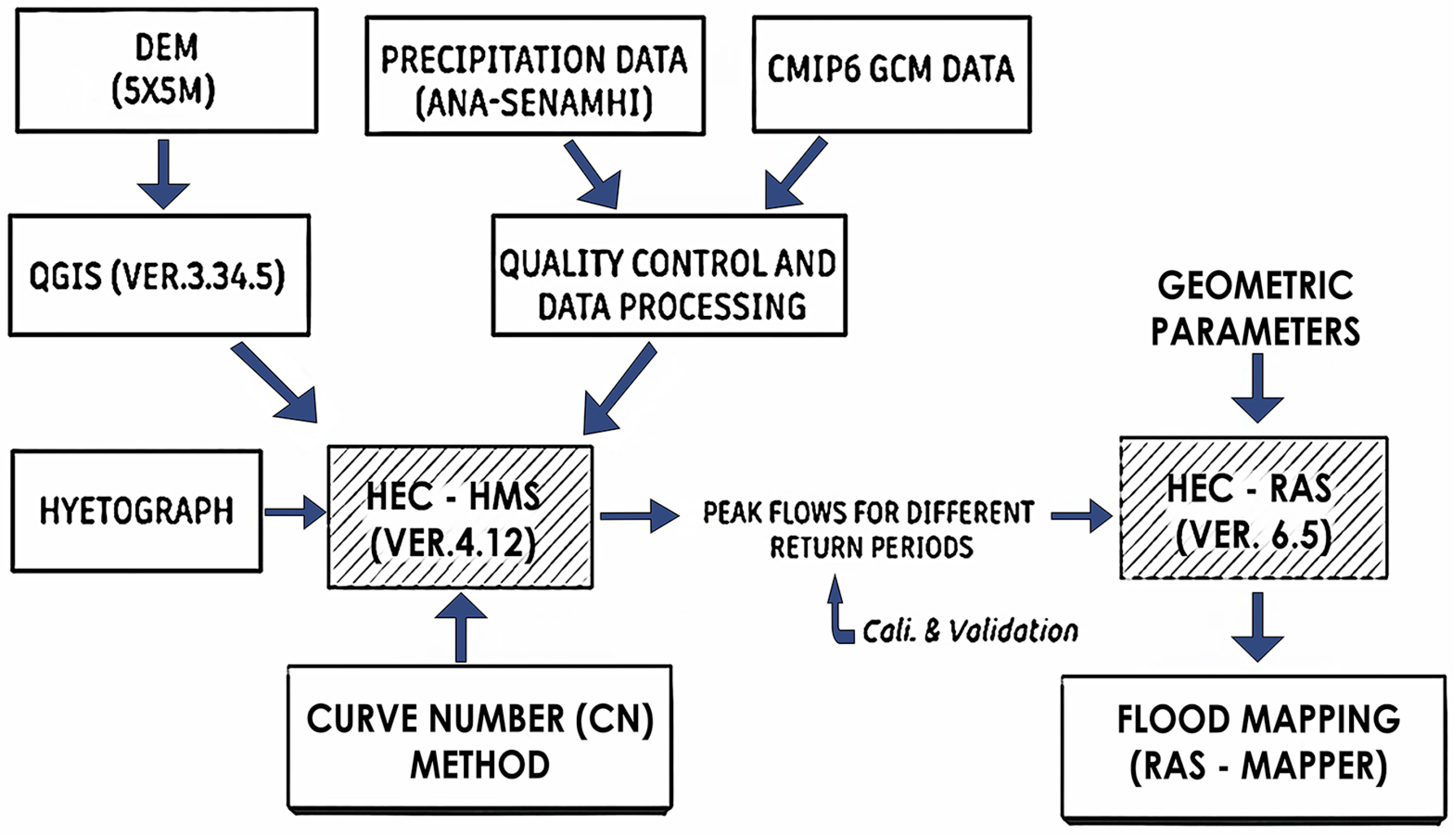
2. Materials and Methods

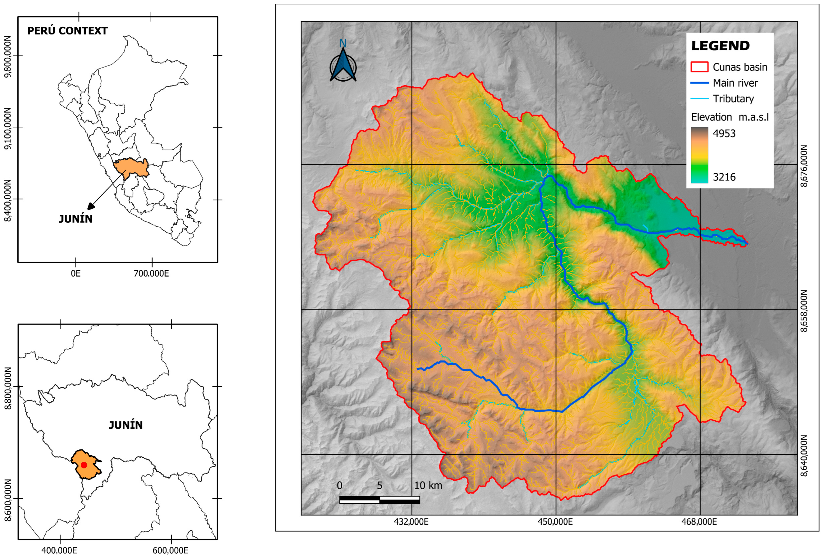
The methodological workflow followed in this study is summarized in Figure 1. Topographic data, obtained from a 5 × 5 m spatial resolution Digital Elevation Model (DEM), were downloaded from the EOSDA LandViewer platform (https://eos.com/find-satellite/, accessed on 15 October 2024), an advanced tool for satellite imagery observation and analysis. This platform enables the search, visualization, and processing of high-resolution Digital Terrain Models (DTMs), optimizing the extraction of relevant information through predefined indices and adjustments. The data were processed in QGIS (v. 3.34.5), while annual maximum daily precipitation data for baseline conditions and Global Climate Model (GCM) CMIP6 projections were obtained from meteorological stations near the study area, managed by the Autoridad Nacional del Agua (ANA) (https://snirh.ana.gob.pe/SNIRHPortal/, accessed on 7 March 2024) and the Servicio Nacional de Meteorología e Hidrología del Perú (SENAMHI) (https://www.gob.pe/senamhi, accessed on 7 March 2024). Subsequently, the data underwent quality control and processing before being integrated into the HEC-HMS model (v. 4.12). Using the Curve Number (CN) method, peak discharges for different return periods were simulated. The hydrological modeling results were then input into the HEC-RAS model (v. 6.5) to perform hydraulic simulations and identify flood-prone areas using RAS-Mapper, enabling a comprehensive assessment of flood hazard in the Cunas River Basin (CRB).

2.1. Study Area

The Cunas River Basin (CRB) is situated in the Junín department (central Peru), approximately between the following coordinates: latitude 11°53′24″–12°25′48″ S and longitude 75°10′12″–75°37′48″ W (WGS 84). It originates in the Cordillera Occidental at 4953 m above sea level (masl), crosses the provinces of Chupaca, Concepción, and Huancayo, and flows into the Mantaro River at approximately 3216 masl. The basin covers an area of 1700.25 km², and its main channel extends 93.79 km in length. The Cunas River is a major tributary of the Mantaro River, which in turn forms part of the Amazon Basin [51].

Precipitation displays a marked seasonal behavior divided into several periods: the wet season features maximum rainfall in December, January, and February, accumulating approximately 346 to 450 mm; from March to May, rainfall decreases moderately, with precipitation recorded between 196 and 281 mm; the dry season occurs between June and August, with minimal precipitation of 37 to 56 mm; from September to November, rainfall increases slightly, reaching values between 185 and 230 mm, indicating a transition toward the wet season [52]. Annually, 83% of precipitation occurs between October and April, with 48% distributed almost equally across January, February, and March [53]. Interannual precipitation variability is approximately 18.65% relative to the mean. Extreme events include a wet period in 1981 (annual precipitation: 920 mm) and a dry period in 1992 (annual precipitation: 400–500 mm) [53].

To obtain topographic information and integrate topographic data derived from 5 m spatial resolution Digital Elevation Models (DEMs), QGIS (v. 3.34.5) software (https://qgis.org/, accessed on 27 March 2024) was used. The drainage network (main channels and tributaries), basin boundaries (precise basin delineation), and altimetry were delineated (Figure 2), and the morphometric properties of the basin were calculated (

Table 1. Main morphometric characteristics of the Cunas River Basin.

Cunas River Basin (CRB)	Indicator	Unit	Value
Morphometric Basin Properties	Area	[km2]	1700.25
	Perimeter	[km]	279.62
	Length	[km]	54.37
	Width	[km]	31.27
	Mean slope	[%]	23.73
	Maximum elevation	[masl]	4953.00
	Minimum elevation	[masl]	3216.00
	Mean elevation	[masl]	4203.82
Main Channel Properties	Length	[km]	93.79
	Length to watershed divide	[km]	98.50
	Highest elevation	[masl]	4532
	Lowest elevation	[masl]	3221
	Mean slope	[%]	1.40%
Drainage Basin Properties	Total drainage length	[km]	2839.16
	Drainage density	[km/km2]	1.67
	Stream order	[-]	5°
	Runoff coefficient	[-]	0.59
Shape Index	Compactness coefficient, Kc	[-]	1.90
	Shape factor, Kf	[-]	0.19

).

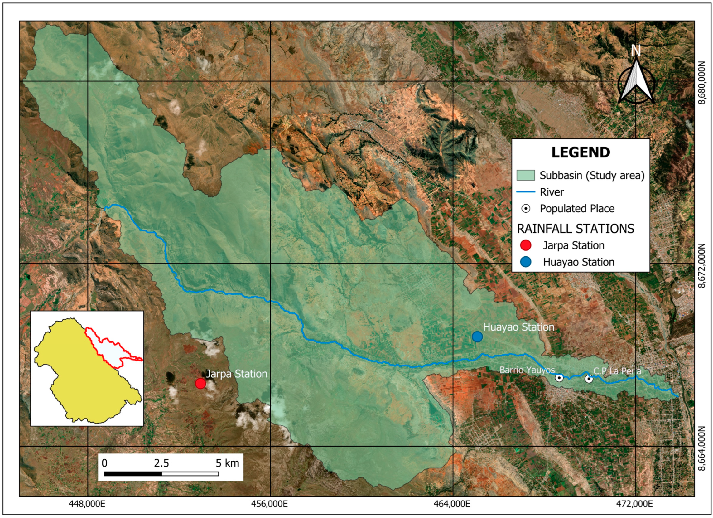
2.2. Micro-Watershed Area

The micro-watershed analyzed in this study is located in the northeast of the study basin. It covers an area of 186.07 km², with a river channel length of 33.31 km and a slope of 1%. The area has two rainfall stations responsible for measuring and recording precipitation amounts, expressed in millimeters (mm). The first is the San Juan de Jarpa station, located at 12°7′28.3″ S latitude, 75°25′54.4″ W longitude, and an altitude of 3660 masl. The second is the Huayao station, located at 12°2′24.7″ S latitude, 75°19′13.8″ W longitude, and an altitude of 3321 masl (Figure 3). Due to the absence of rain gauge stations within the study micro-watershed, a nearby station such as San Juan de Jarpa is used. Although it is located outside the micro-watershed boundaries, its inclusion is based on its proximity to the micro-watershed limit, and its records influence the study area due to the homogeneous climatic conditions present in that part of the micro-watershed. This area of influence will be validated later.

2.3. Hydrological Study Under Baseline Conditions

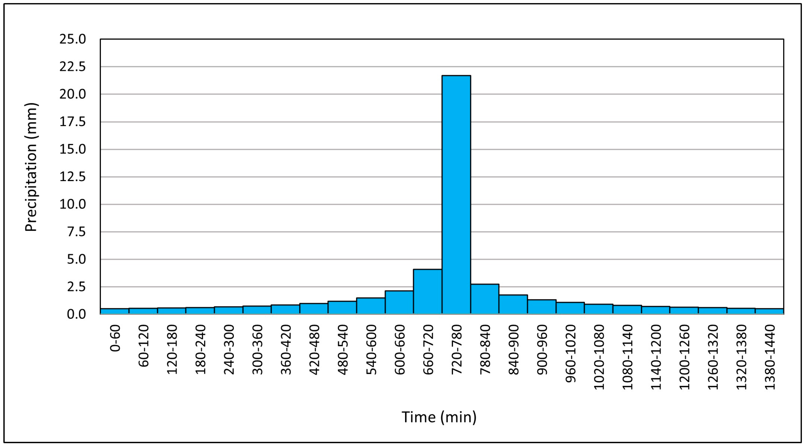
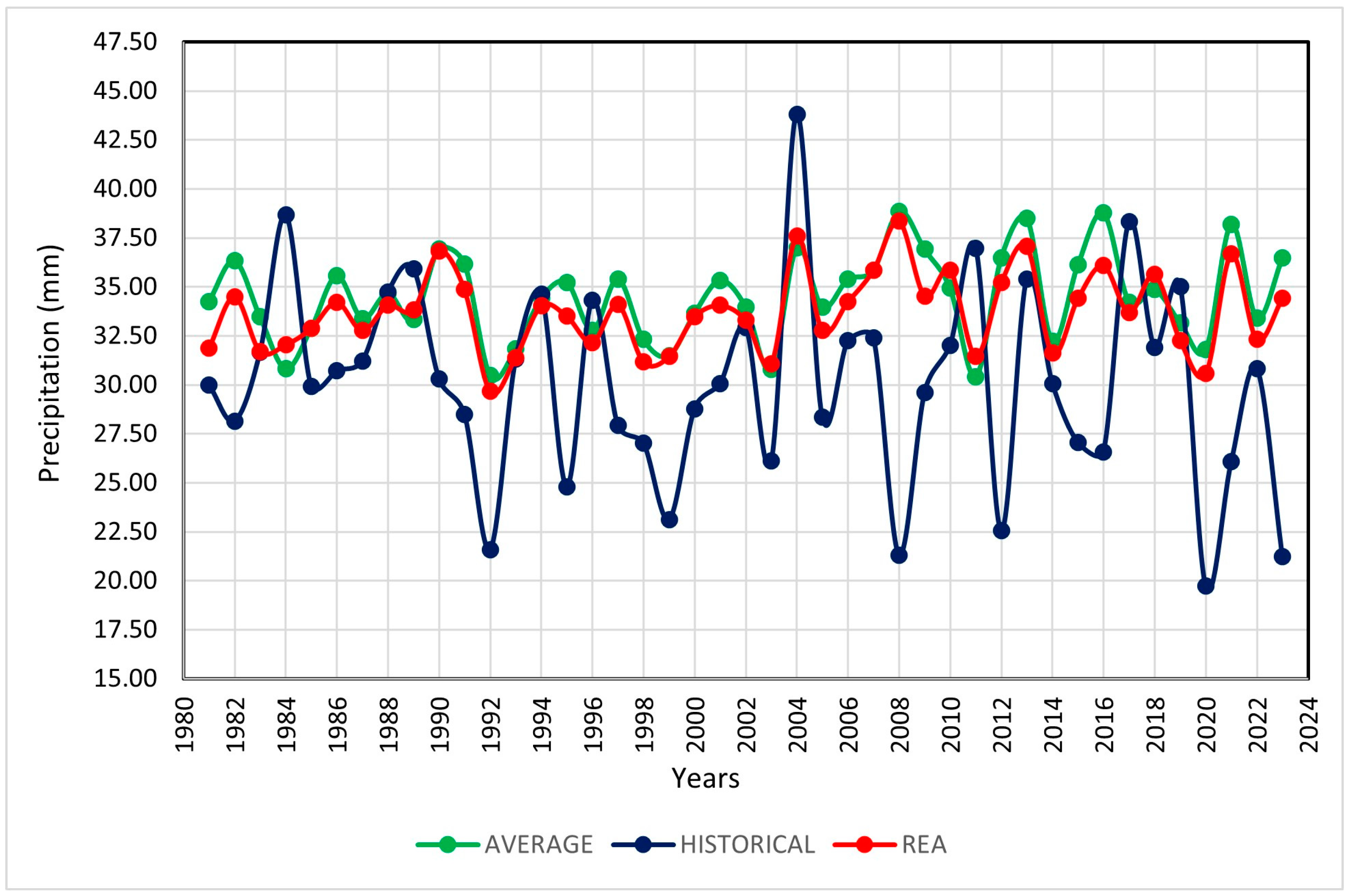
2.3.1. Precipitation Influence and Analysis

As previously mentioned, rainfall measurements and records were obtained from the San Juan de Jarpa and Huayao stations. This data were provided by the Servicio Nacional de Meteorología e Hidrología del Perú (SENAMHI) (https://www.gob.pe/senamhi, accessed on 7 March 2024) and the Autoridad Nacional del Agua (ANA) (https://snirh.ana.gob.pe/SNIRHPortal/, accessed on 7 March 2024), two key Peruvian agencies responsible for delivering reliable and accessible meteorological, hydrological, and climatic information. Historical daily maximum precipitation data from 1974 to 2023 were considered.

To spatially distribute maximum and average precipitation across the basin equitably, the Thiessen polygon method was applied. This method constructs polygons—formed by perpendicular bisectors between pairs of adjacent stations—to represent the influence area of each station [54]. The influence area of the Huayao Station in the micro-watershed is 108.02 km², while that of the San Juan de Jarpa Station is 77.45 km². The corresponding coefficients, expressed as percentages using Equation (1), are 41.62% and 58.38%, respectively.

$$P_p=\sum _{i=1}^n{P}_{i}x{\displaystyle \frac{A_i}{A_t}}$$

(1)

where $P_p$ is the weighted or mean precipitation in the basin (in mm), $A_i$ is the area of the polygon corresponding to station $i$ (in km²), $A_t$ is the total area (in km²), $P_i$ is the precipitation measured at the station (in mm), and $n$ is the total number of stations.

An adjustment of outliers in precipitation data was performed using the Water Resources Council (WRC) method, which identifies data points that deviate significantly from the trend of the remaining dataset [55]. According to this statistical outlier analysis, with a significance level of 10% for a normal distribution, the precipitation data fall within the trend range, establishing a more robust distribution of the historical records [56].

To assess temporal trends in annual maximum daily precipitation, the Mann–Kendall (MK) test [57,58,59] was applied, which is based on the sequential comparison of the values in a time series, considering the hypothesis of series stability. According to the analysis performed with the free software TREND (v. 1.0.2) [60], no statistically significant trend was observed in the precipitation series of the CRB.

Through the Kolmogorov–Smirnov goodness-of-fit tests [61], it was determined that the Pearson Type III distribution provides the best fit (99.63%) for calculating annual maximum precipitation values for return periods of 2, 5, 10, 25, 50, 100, 139, 200, and 500 years. Additionally, a fixed interval factor of 1.13 was applied to the maximum precipitation values for each of the specified return periods to correct and adjust these values, improving their representativeness in the hydrological analysis [62].

Subsequently, IDF curves were calculated using the Dyck–Peschke model [63], which, through multiple regression analysis, derived rainfall intensities for the aforementioned return periods (Figure 4). This enabled the development of a hyetograph via the Alternating Block Method, used to analyze the temporal distribution of rainfall across different return periods [64]. The hyetograph displays rainfall intensity at specific 60-min time intervals, providing critical input for hydrological modeling. Likewise, a total duration of 1440 min was considered, aiming to comprehensively capture the temporal distribution of extreme precipitation events characteristic of the study region. This methodological decision is based on the approach proposed by the Manual de Diseño de Obras de Drenaje of the Ministerio de Transportes y Comunicaciones del Perú (MTC) [65], which includes the use of this duration in the analysis of design storms for hydraulic structures, and is also aligned with the hydrological procedures recommended by SENAMHI. This approach allowed us to accurately estimate both the intensity and total volume of the event, which is crucial for the design of drainage infrastructure, flood control, and territorial planning. Below, the design precipitation hyetograph for a 139-year return period is shown (Figure 5).

It is important to emphasize that this study primarily focuses on a 139-year return period, as the provided data are intended to serve as the basis for designing riverbank defense structures, in accordance with the guidelines established by the Ministerio de Transportes y Comunicaciones (MTC) [65]. This return period is critical to ensure that such infrastructure, designed for future resilience, can effectively mitigate flooding risks based on extreme events with a specific probability of occurrence [65].

2.3.2. Estimation of Maximum Discharge (Qm) Using HEC-HMS

To estimate maximum discharge under baseline conditions for different return periods, HEC-HMS software (v. 4.12) (https://www.hec.usace.army.mil/software/hec-hms/, accessed on 28 March 2024) was employed. The Soil Conservation Service (SCS) Curve Number (CN) method calculates rainfall excess as a function of cumulative precipitation, land cover, land use, and antecedent soil moisture [66]. This method was selected for its simplicity, predictability, stability, and reliance on a single variable, CN, to predict the rainfall–runoff relationship, as well as its responsiveness to key basin properties influencing runoff, such as soil type, land use, surface condition, and antecedent moisture condition [67]. Furthermore, it provides a rapid method to estimate changes in runoff resulting from land use modifications [68]. CN values range from 0 to 100, where higher values indicate greater runoff and reduced infiltration. For calculating the Curve Number (CN), data from thematic CN maps developed by the Autoridad Nacional del Agua (ANA) (https://snirh.ana.gob.pe/onrh/, accessed on 7 March 2024) were used. These data were processed in QGIS to delineate the specific boundaries of our sub-basin. Equation (2) was applied to compute the CN, yielding a value of 92, which serves as a key input for the hydrological model.

$$CN={\displaystyle \frac{\sum {CN}_{i}x{A}_i}{\sum A_i}}$$

(2)

where $CN$ is the average curve number of the basin, ${CN}_i$ is the curve number of each area or sub-basin $i$, $A_i$ is the area corresponding to each ${CN}_i$ (in km²), and $\sum A_i$ is the total area of the basin (in km²).

The time of concentration (Tc) is the time required for the entire watershed to contribute to runoff at the point of interest for hydraulic design. It is calculated as the time it takes for runoff to flow from the hydraulically most remote point of the drainage area to the watershed outlet [69]. The procedures used to estimate Tc depend on several factors, including watershed characteristics (particularly drainage area) and available morphometric parameters [70]. Different established methods for calculating Tc were compared, ultimately highlighting and applying only three of them, whose variability (Min. Var. and Max. Var.) within the acceptable range (5.50 to 8.64) was considered valid. While it is true that the methods used were originally developed and calibrated for specific regions in other countries, such as Giandotti (Italy), Kirpich (United States), and California Culverts Practice (United States), the manual of the Ministerio de Transportes y Comunicaciones (MTC) allows the use of these methods [65]. Moreover, the decision to use and average these methods was made because each considers different factors, and applying them allows for a better representation of the watershed’s hydrological characteristics, such as topography, climate, roughness, and slopes, thereby reducing the inherent bias of each one [71,72]. The average Tc value calculated for the studied hydrological unit is 6.22 h (

Table 2. Analysis of methods for calculating the time of concentration (Tc).

Method Used	Calculated Tc (h)	Min. Var. (h)	Max. Var. (h)	Accepted	Valid Tc (h)
Giandotti	7.11	5.50	8.64	Yes	7.11
Kirpich	5.77	5.50	8.64	Yes	5.77
California Culvers Practice	5.78	5.50	8.64	Yes	5.78
Average calculated Tc for the studied hydrological unit					6.22

).

Similarly to the time of concentration (Tc), the MTC recommends using a 0.6 factor to determine the lag time (Tp) [65], which, in this case, is 3.73 h. This method has been adopted due to the complex characteristics of Andean basins in Peru, allowing the SCS model to be adapted more practically without requiring specific calibrations.

2.3.3. Simulation of the Cunas River Behavior Using HEC-RAS

The HEC-RAS model, developed by the U.S. Army Corps of Engineers (USACE), employs mass and momentum conservation equations to analyze flow dynamics and assess flood risks. HEC-RAS (v. 6.7) was used to simulate the behavior of the Cunas River, enabling the prediction and evaluation of flood magnitude and impact in the study area under both baseline conditions and a future climate change scenario.

The Cunas River geometry was imported in ESRI Shapefile format. The channel line was traced following the axis of the natural channel and was used to define the cross-sections. Bank Lines demarcated the main channel, while flow paths on the floodplain delineated overflow boundaries. Cross-sections were drawn perpendicular to the water flow direction and extended beyond the flow lines’ limits. A first simulation was performed, where 23 cross-sections were created, each 600 m wide and spaced 300 m apart, where the overflow of the river under the influence of climate change demonstrated the need for a wider limitation. Consequently, through multiple simulations with adjusted dimensions, a new overflow boundary was implemented to encompass greater flood-prone areas. The cross-sections were strategically repositioned in zones exhibiting more severe flooding, maintaining an average 300-m spacing along the Cunas River channel to ensure uniform distribution, a critical factor for accurate topographic representation. For HEC-RAS computations, flow data incorporating maximum discharge values calculated for a 139-year return period were input.

Manning’s roughness coefficients, selected through field observations and accounting for the characteristics of the main channel and both banks (right and left), were input based on the tables proposed by Ven T. Chow [73] (

Table 3. Manning’s roughness coefficients selected for each reach of the main channel.

Reach (m)	Channel Type and Description	n
6899.7–6599	Sparse shrubs and trees	0.055
6599–6300.3	Sparse shrubs and trees	0.055
6300.3–5999	Sparse shrubs and trees	0.055
5999–5701	Sparse shrubs and trees	0.055
5701–5399	Sparse shrubs and trees	0.055
5399–5100.2	Grasslands, no shrubs, short grass	0.030
5100.2–4799	Scattered shrubs, dense undergrowth	0.050
4799–4500	Cleared land with trees and abundant saplings	0.060
4500–4199.9	Mature row crops	0.035
4199.9–3903	Mature row crops	0.035
3903–3600	Scattered shrubs, dense undergrowth	0.050
3600–3300	Grasslands, no shrubs, short grass	0.030
3300–2998	Mature row crops	0.035
2998–2697	Clear, straight stream with rock mounds and vegetation	0.035
2697–2397	Clear, straight stream with rock mounds and vegetation	0.035
2397–2099	Mature row crops	0.035
2099–1799	Clear, straight stream with rock mounds and vegetation	0.035
1799–1498	Clear, straight stream with rock mounds and vegetation	0.035
1498–1201	Clear, straight stream without mounds or deep pools	0.030
1201–899	Clear, straight stream without mounds or deep pools	0.030
899–598	Mature row crops	0.035
598–298	Clear, straight stream with rock mounds and vegetation	0.035

). The calculated coefficients vary across river reaches, as illustrated in Figure 6. The downstream slope was derived from longitudinal profile data, with an elevation difference of 64.80 m between upstream and downstream reaches and a reach length of 6590.33 m, yielding an approximate slope of 1% from morphometric parameter calculations. Following geometry definition, the data were imported into HEC-RAS.

2.4. Hydrological Study Under Climate Change Conditions

2.4.1. Global Climate Models (GCMs) from CMIP6

The simulated climate data from Global Climate Models (GCMs) of CMIP6 were analyzed using the VECC (Visor Escenarios de Cambio Climático) tool from the Mantaro Basin Observatory, provided by the Autoridad Nacional del Agua (ANA) (https://observatoriomantaro.ana.gob.pe/es-es, accessed on 15 March 2024). VECC is a decision-support tool for addressing climate change impacts in this region, designed to integrate climatic, hydrological, and socioeconomic information while enabling visualization of climate data simulated by CMIP6 Global Climate Models (GCMs) that contributed to the latest IPCC report.

For assessing future precipitation trends, this study utilized 10 GCMs from CMIP6 (CanESM5, CNRM-CM6-1, CNRM-ESM2-1, GFDL-ESM4, IPSL-CM6A-LR, MIROC6, MPI-ESM1-2-HR, MRI-ESM2-0, UKESM1-0-LL y ACCESS-ESM1-5) (

Table 4. List of the 10 CMIP6 GCMs used in this study.

N°	GCM Name	Institution	Country	Spatial Resolution
M1	CanESM5	Canadian Centre for Climate Modelling and Analysis (CCCma)	Canada	2.81° × 2.81°
M2	CNRM-CM6-1	Centre National de Recherches Météorologiques (CNRM)	France	1.4° × 1.4°
M3	CNRM-ESM2-1	Centre National de Recherches Météorologiques (CNRM)	France	2.8° × 2.8°
M4	GFDL-ESM4	Geophysical Fluid Dynamics Laboratory (GFDL)	USA	1° × 1°
M5	IPSL-CM6A-LR	Institut Pierre-Simon Laplace (IPSL)	France	2.5° × 2.5°
M6	MIROC6	Modeling and Information Research on Climate (MIROC), University of Tokyo, National Institute for Environmental Studies, and Japan Agency for Marine-Earth Science and Technology	Japan	1.4° × 1.4°
M7	MPI-ESM1-2-HR	Max Planck Institute for Meteorology (MPI-M)	Germany	0.94° × 0.94°
M8	MRI-ESM2-0	Meteorological Research Institute (MRI)	Japan	1.4° × 1.4°
M9	UKESM1-0-LL	UK Met Office Hadley Centre	UK	1.25° × 1.25
M10	ACCESS-ESM1-5	Australian Community Climate and Earth-System Simulator (ACCESS), Commonwealth Scientific and Industrial Research Organisation (CSIRO), Bureau of Meteorology	Australia	1.875° × 1.25°

), under the SSP5-8.5 scenario for the period 2023–2100.

This study adopts the SSP5-8.5 scenario from the Coupled Model Intercomparison Project Phase 6 (CMIP6) to assess climate change impacts in the study basin. This scenario represents a high-emission pathway characterized by rapid fossil fuel-driven economic growth and accelerated technological development, resulting in sustained increases in greenhouse gas emissions [74], projecting an additional radiative forcing of 8.5 W/m² by the year 2100, potentially increasing global temperatures by 2.42–5.64 °C with significant implications for flood risk [75].

2.4.2. RAIN4PE Product

The historical and projected precipitation data from the 10 GCMs were specifically adjusted for the region and study area through a bias correction and statistical downscaling process, using local data as a reference, including the RAIN4PE product for precipitation.

RAIN4PE is a novel gridded daily precipitation dataset for Peru and Ecuador, developed by merging precipitation data from multiple sources: the Climate Hazards Group’s Infrared Precipitation with Satellites (CHIRPS) [76], ERA5 reanalysis [77], and ground-level precipitation adjusted for terrain elevation using random forest regression; additionally, the dataset incorporates hydrological correction using streamflow data in basins where precipitation is underestimated, applying inverse hydrology [78]. Therefore, RAIN4PE serves as a valuable tool for hydrometeorological applications in the region, including hydrological modeling and assessment of hydroclimatic extremes such as droughts and floods (Figure 7).

Figure 7 presents the workflow diagram of the RAIN4PE product, whose methodology was structured into three complementary stages. First, a multi-source precipitation data fusion was performed using the Random Forest (RF) algorithm, incorporating point observations and covariate variables (CHIRP, ERA5, elevation, and local databases), which allowed for the generation of a corrected daily dataset known as RAIN4PE. Subsequently, a hydrological adjustment of the daily precipitation data was applied using the SWAT model, calibrated with observed streamflow records. In this stage, a hydrological correction factor (BCF) was introduced and applied to the precipitation dataset (Pg × BCF), enabling improved streamflow (Q) simulation until objective fit criteria (OFs) were met. Finally, the hydrological performance of the calibrated model was evaluated during the calibration and validation periods by calculating goodness-of-fit metrics (GOFs), in order to validate the consistency and applicability of the corrected dataset for hydrological modeling purposes [78]. The RAIN4PE dataset covers the land surface between 19° S–2° N and 82–67° W with a daily spatial resolution of 0.1°, spanning the period from 1981 to 2015 [78].

2.4.3. Reliability Ensemble Averaging (REA)

REA (Reliability Ensemble Averaging) is a method used to calculate the mean, uncertainty range, and a reliability measure of simulated climate changes at subcontinental scales from ensembles of different atmosphere–ocean General Circulation Model (AOGCM) simulations [46]. This method employs a weighted average of simulations, where each model’s contribution to the forecast results is determined by its assigned weight. These weights are derived from two key criteria: the model’s performance in historical simulations, and its convergence with other models in future projections [79]. The REA method, widely employed in previous studies under various approaches [80,81], enhances the accuracy of climate projections by integrating results from different CMIP6 models under the SSP5-8.5 climate scenario. To apply the REA method, each model projection $i$ from the ensemble of 10 GCMs is assigned a reliability factor $R_i$ calculated using Equation (3).

$$R_i=R_{B,i}\times R_{D,i}=\left({\displaystyle \frac{\epsilon }{\left|B_i\right|}}\right)\times \left({\displaystyle \frac{\epsilon }{\left|D_i\right|}}\right)$$

(3)

where $B_i$ and $D_i$ represent the performance and convergence measures, respectively, for model $i$. The parameter $\epsilon$ denotes the observational variability, expressed as the difference between maximum and minimum values. The performance factor $R_{B,i}$ ranges from 0 (for a low-performance model) to 1, if $\left|B_i\right|$ is less than $\epsilon$. Similarly, the convergence factor $R_{D,i}$ ranges from 0 (for outlier projections) to 1, if $\left|D_i\right|$ (the difference between the projection and the REA mean) is less than $\epsilon$.

The advantage of using the REA method lies in its simultaneous consideration of both performance (based on a model’s prediction quality) and convergence (determined by its position within an ensemble of projections) [82]. Therefore, when applying this method, the primary objective is to assign a weight to each of the 10 GCMs and combine the projections through weighted averaging, thereby maximizing precision, reducing uncertainty, and enhancing reliability in precipitation projections for the region [46]. Figure 8 presents an analysis with uniform weighting for each model, where validity and predictive capacity are equal across all models. It further illustrates the variability in weights obtained through REA method application, demonstrating that certain models are more capable of improving future climate conditions and discarding the idea that assigning the same weight to each model (averaging) is better. Figure 9 compares a time series of annual maximum precipitation, presenting historical precipitation data, the mean values from the 10 GCMs, and the REA-adjusted values. The results highlight the REA method’s performance in combining and correcting modeled values by closely tracking the historical trend while smoothing extreme fluctuations.

2.4.4. Performance Evaluation Methods

The hydrological model performance in the CRB for hydrological simulation is determined using the Nash–Sutcliffe Efficiency (NSE) [83]. The NSE ranges from −∞ to 1, where values approaching 1 indicate excellent model fit, Equation (4). The absolute fit differences are quantified using the Mean Absolute Error (MAE, Equation (5)) and Root Mean Square Error (RMSE, Equation (6)), where a value of 0 indicates perfect agreement. The correlation coefficient (R²) determines the degree of correlation between simulated and measured data, ranging from −1 to 1, where values closer to 1 indicate a better fit, Equation (7). The Percent Bias (PBIAS) measures the model’s overestimation or underestimation, Equation (8).

$$NSE=1-{\displaystyle \frac{{\sum }_{i=1}^n{(O_i-S_i)}^2}{{\sum }_{i=1}^n{(O_i-\overline{O})}^2}}$$

(4)

$$MAE={\sum }_{i=1}^n{\displaystyle \frac{\left|O_i-S_i\right|}{n}}$$

(5)

$$RMSE=\sqrt{{\sum }_{i=1}^n{\displaystyle \frac{{(O_i-S_i)}^2}{n}}}$$

(6)

$$R^2={\left({\displaystyle \frac{{\sum }_{i=1}^n\left(O_i-\overline{O}\right)\left(S_i-\overline{S}\right)}{\sqrt{{\sum }_{i=1}^n{\left(O_i-\overline{O}\right)}^2}\sqrt{{\sum }_{i=1}^n{\left(S_i-\overline{S}\right)}^2}}}\right)}^2$$

(7)

$$PBIAS=\left[{\displaystyle \frac{{\sum }_{i=1}^n(O_i-S_i)}{{\sum }_{i=1}^n{O}_i}}\right]\times 100$$

(8)

where $O_i$ represents the observed discharge (m³/s), $S_i$ is the simulated discharge (m³/s), $\overline{O}$ is the mean observed discharge (m³/s), $\overline{S}$ is the mean simulated discharge (m³/s), and $n$ is the number of observations.

For model calibration, observed discharge data from the Angasmayo hydrometric station were used, while validation was performed using observed discharge data from the Pilcomayo hydrometric station, both covering the period from 1984 to 2023. The objective was to adjust the model parameters until achieving a satisfactory agreement between observed and simulated discharge values [84,85].

3. Results

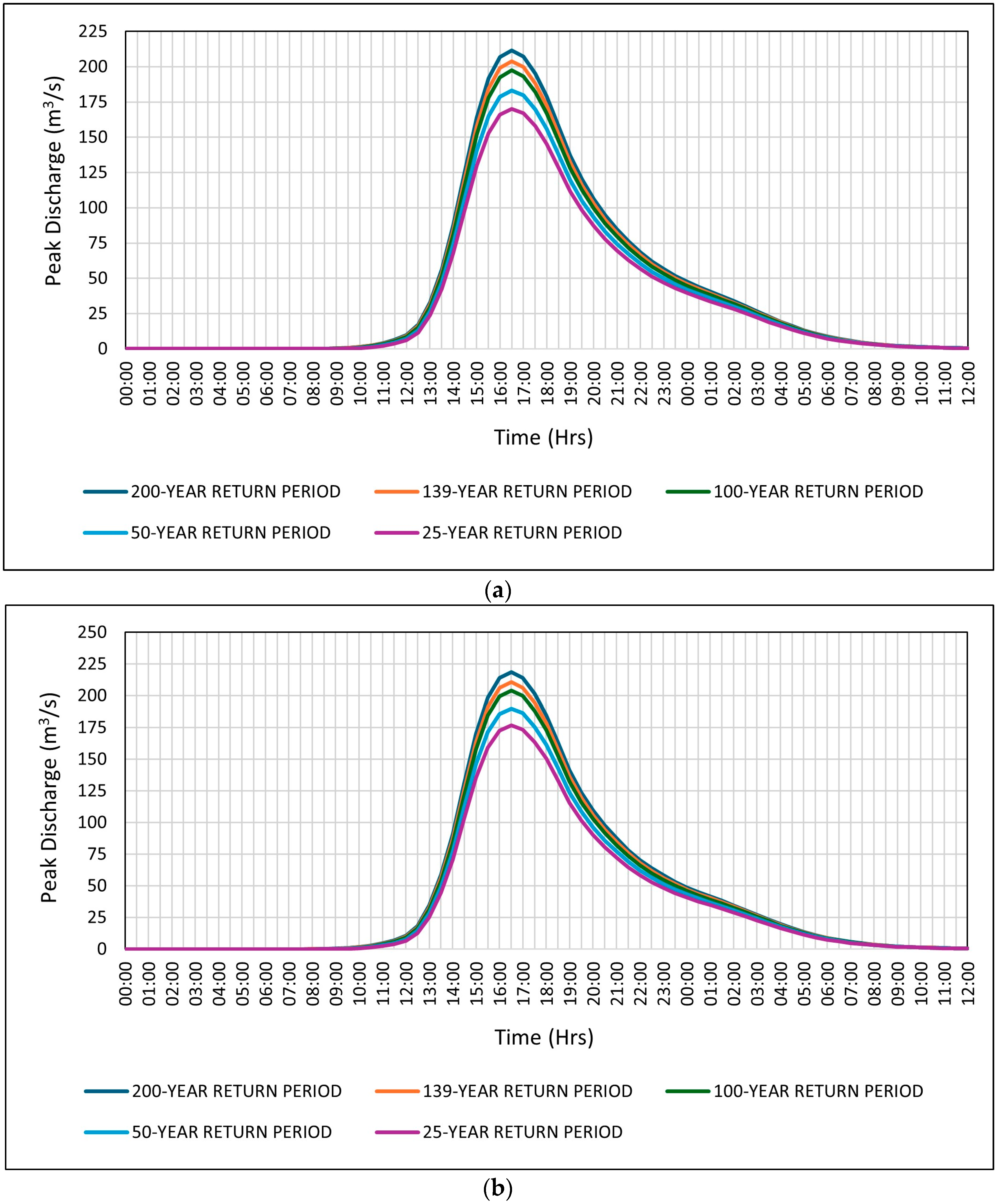
3.1. Calculation of Maximum Design Discharge Using HEC-HMS

Following the hydrological analysis of the Cunas River using the HEC-HMS model, discharge values were obtained for the two analyzed scenarios (baseline conditions and under climate change influence) for return periods of 25, 50, 100, 139, and 200 years. The main result of the analysis focused on the 139-year return period, due to the approach the study presented.

Table 5. Comparison of peak discharges under the two analyzed conditions.

Return Period (Years)	Peak Discharge (m3/s)
	Baseline Conditions	Climate Change Conditions
25	170.20	176.80
50	183.20	190.00
100	197.70	204.00
139	203.90	210.90
200	211.60	218.70
500	232.20	239.40

shows that the peak discharge for a 139-year return period under normal conditions was 203.90 m³/s, while under climate change conditions, it reached 210.90 m³/s, indicating a 3.32% flow increase attributable to climate change effects. This rise in peak discharges underscores the growing influence of the climate scenarios applied in our analysis, highlighting the critical importance of considering climate change as a key variable when planning preventive measures against hydrological risks such as flooding.

On the other hand, to better manage and extend the scope of the obtained results, hydrographs (flow rate–time) were obtained. These graphically represent the variation in the flow rate of the Cunas River as a function of time, given in hours, in response to the previously analyzed precipitation events. These hydrographs were the result of analyses conducted in HEC-HMS, where, after processing the data, the graphs were generated independently for each return period, with time measured in hours. Subsequently, after adjusting the information, the hydrographs shown in Figure 10 were obtained for return periods of 25, 50, 100, 139, and 200 years. These hydrographs are presented under two conditions: normal conditions (Figure 10a) and with the presence of climate change (Figure 10b), where the color variation refers to each return period. While it is true that these hydrographs arise together with the flow rates obtained in Table 5, the importance of these graphs lies in providing a better understanding of the hydraulic process as a function of time.

Figure 10 displays the hydrographs of peak discharge (m³/s) versus time at half-hour intervals for the two conditions studied and for the previously established return periods.

Figure 10a shows the hydrograph under baseline conditions, where the peak discharge for the 139-year return period reaches 203.90 m³/s, occurring at 16:30 h. On the other hand, Figure 10b presents the hydrograph under climate change conditions, where the temporal flow distributions exhibit higher peaks compared to baseline conditions. For the 139-year return period, the peak discharge reaches 210.90 m³/s, also at 16:30 h, representing a 3.32% increase in discharge.

This indicates that, in both cases, during this time interval, sufficient water has accumulated to generate the highest flow of the event at this specific hour, and the previously determined time of concentration is a contributing factor to this result.

3.2. Hydrological Model Calibration and Validation

The hydrological model was calibrated and validated using historical observed discharge data from the Angasmayo (calibration) and Pilcomayo (validation) hydrometric stations for the 1984–2023 period. Performance metrics are detailed in

Table 6. Model calibration and validation.

Type	Period Event	NSE	MAE	RMSE	R2	PBIAS
Calibration	1984–2023	0.939	−0.129	5.418	0.998	−0.001
Validation	1984–2023	0.921	−3.337	6.095	0.998	0.015

.

The coefficient of determination (R²) reached a value of 0.998 for both calibration and validation, indicating a strong linear correlation between observed and simulated discharges. This high R² suggests that the model effectively captures the overall trend of the data across the evaluated period.

The Percent Bias (PBIAS) exhibited very low values: −0.001 for calibration and 0.015 for validation. These near-zero values reflect the model’s absence of systematic bias (i.e., no consistent overestimation or underestimation of discharges), demonstrating its capacity to simulate the water balance accurately and reliably.

These positive performance metrics confirm the hydrological model’s effectiveness in representing the average flow behavior of the Cunas River Basin (CRB), providing a robust foundation for subsequent analyses.

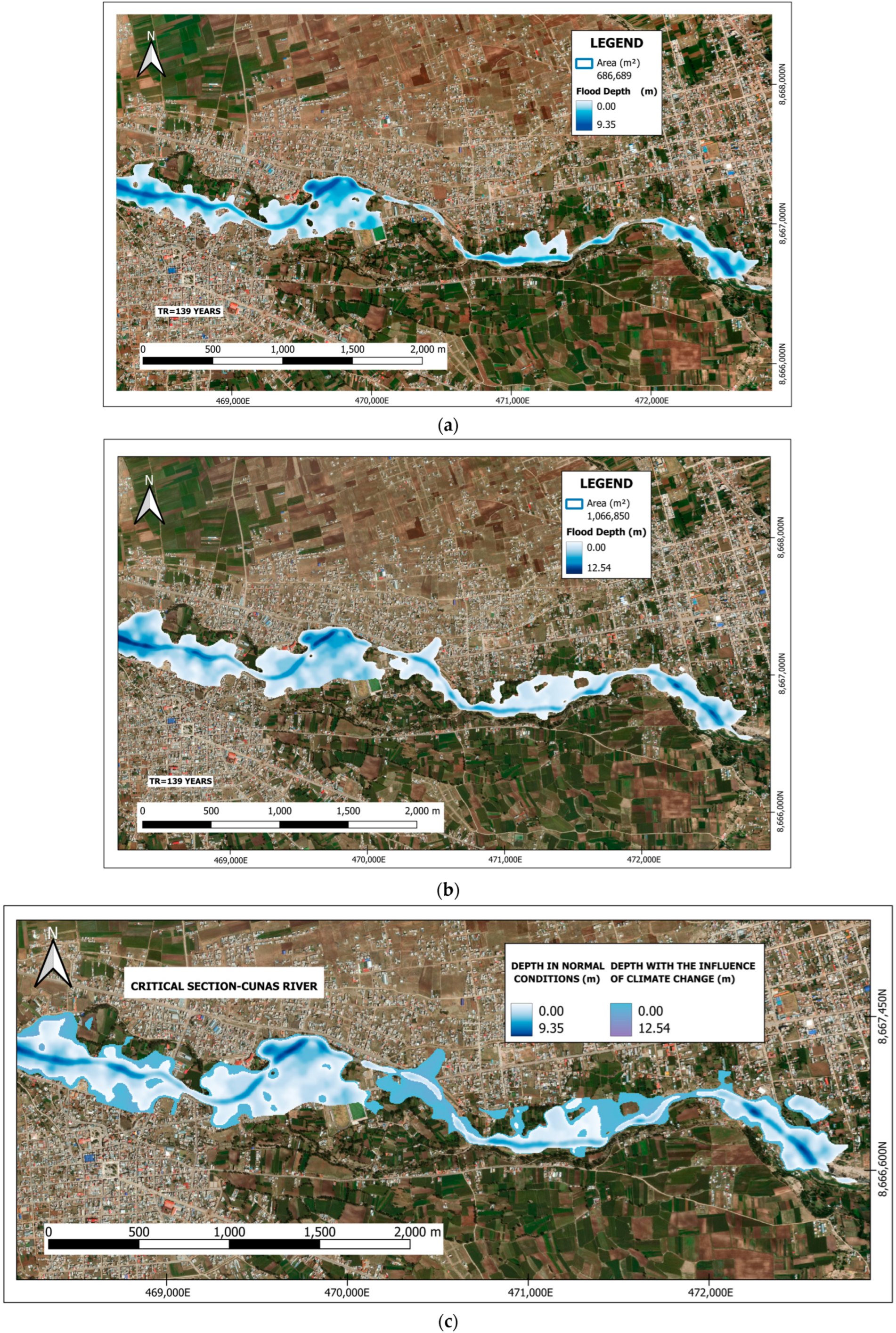
3.3. Flood Simulation (Flooded Areas and Sections)

Using the previously obtained hydrological data and the HEC-RAS software, the simulation of flooded areas and sections of the Cunas River was conducted for a 139-year return period (Figure 11), under baseline conditions (Figure 11a) and with climate change influence (Figure 11b). Additionally, these two simulations were overlaid into a single map to provide a better perspective between both conditions (Figure 11c).

To delineate flood-prone areas in the Cunas River basin, specific hydraulic thresholds were applied in HEC-RAS. Flood discharges were simulated for return periods of 25, 50, 100, 139, and 200 years, derived from hydrological modeling in HEC-HMS under CMIP6 climate projections. The 139-year return period was selected for flood simulations under both baseline conditions and climate change scenarios. As a classification criterion, areas with water depths equal to or exceeding 0.1 m were considered flooded, in accordance with standard risk assessment practices. Upstream boundary conditions were defined based on peak discharges generated by HEC-HMS for the 139-year return period.

This approach enabled a detailed characterization of flood-susceptible zones, integrating both hydrological variables and established technical criteria.

Figure 11a displays the flood model under baseline conditions, with a total inundated area of 686,689 m². The simulation identified approximately 324 households at risk, of which 76 households were classified as directly highly vulnerable and 248 as less vulnerable, primarily in the Centro Poblado La Perla and part of Barrio Yauyos, located in the province of Chupaca. Additionally, 115 agricultural plots along both banks of the Cunas River would be impacted. These lands, dedicated to crop production (potatoes, corn, barley, wheat, quinoa) and livestock rearing (cows, pigs, sheep, chickens, hens), cover a total area of 183,892 m², representing 26.78% of the total flooded zone. Critical infrastructure at risk includes educational institutions, public facilities, recreational areas, the Chupaca General Cemetery, the Chupaca Municipal Stadium, and key transportation routes such as Eternidad Road, which provides direct access to the province of Chupaca.

Figure 11b displays the flood model under climate change influence, with a total inundated area of 1,066,850 m². The simulation identified approximately 462 households at risk, of which 105 households were classified as directly highly vulnerable and 357 as less vulnerable, primarily in Centro Poblado La Perla and Barrio Yauyos, located in the province of Chupaca. Additionally, 147 agricultural plots along both banks of the Cunas River would be impacted. These lands, dedicated to crop production (potatoes, corn, barley, wheat, quinoa) and livestock rearing (cows, pigs, sheep, chickens, hens), cover a total area of 255,620 m², representing 23.96% of the total flooded zone. Critical infrastructure at risk includes educational institutions, public facilities, recreational areas, the Chupaca General Cemetery, the Chupaca Municipal Stadium, and tourist and rural recreational sites. Urban areas such as Raymondi and Los Ángeles would also be significantly affected, along with key transportation routes like Eternidad Road (providing direct access to Chupaca province) and the main road connecting to Yauyos.

Figure 11c displays the overlaid flood extents from both scenarios, revealing a 35.63% increase in inundated area under climate change influence compared to baseline conditions. This expansion is most pronounced in peripheral zones of Centro Poblado La Perla and Barrio Yauyos, where flat topography facilitates water flow propagation. The figure also illustrates flood depth levels in critical zones for both scenarios, with color intensity corresponding to depth. The maximum flood depth reaches 9.35 m under baseline conditions and 12.54 m under climate change influence.

When comparing both events, there is a significant variation in the extent of the flooded areas. On one hand, when simulating under baseline conditions, there are less vulnerable flooded zones with a moderate impact on urban areas. On the other hand, when including the effect of climate change, a considerable increase in flooded areas is observed, also affecting main roads such as those providing access to the province of Chupaca, with more severe future projections. These projections would imply that the floods affect, on one hand, many more homes in the Centro Poblado La Perla and the Barrio Yauyos, and on the other hand, the main road called Coronel Parra, located on the left bank of the Cunas River, which provides access to the province of Chupaca and the district of Huáchac.

The simulation conducted with HEC-RAS also enabled the visualization of cross-sectional profiles along the entire length of the Cunas River. This provided detailed insights into the river’s geometry and elevation variations across defined reaches, as well as the water flow behavior at varying widths and depths.

Figure 12 primarily displays the most critical cross-sections (C.S. 5100.2) within the analyzed reach of the Cunas River for a 139-year return period under two scenarios: baseline conditions (Figure 12a) and climate change influence (Figure 12b). In both cases, the river at this cross-section exhibits a U-shape, with the left bank significantly higher than the right bank, reflecting the Cunas River’s distinct topographic characteristics.

Figure 12a shows that the riverbank elevation is 3236.72 masl, while under baseline conditions, flooding reached 3238.65 masl, indicating a water level rise of 1.93 m.

Figure 12b, under the influence of climate change and with the same riverbank elevation (3236.72 masl), shows that flooding reached 3241.50 masl, corresponding to a water level rise of 4.78 m.

The flood height increase under climate change influence is 2.85 m compared to baseline conditions.

This simulation also reflects the progressive flood capacity buildup over time, driven by turbulent mass-removal flows and laminar flows with significant potential to erode accumulated materials along the channel banks and deposit sediments on the riverbed along its course. These processes cause the river channel margins to expand progressively over time. Furthermore, the absence of preventive and mitigation measures—such as riverbank defense structures (levees, gabions, retaining walls, etc.)—renders the adjacent population increasingly vulnerable to such events.

4. Discussion

Following the assessment of climate change under the 10 GCMs from CMIP6, the model initially projects a 3.32% increase in discharge when incorporating climate change, which is directly attributed to extreme precipitation events. These findings align with a study [19] which evaluated the response under the RCP 8.5 climate change scenario and reported projections of an 8.14% increase in precipitation and a 12.6% rise in streamflow for a high-Andean basin in Peru. Furthermore, projected streamflows under the RCP 8.5 scenario exhibit a significant increase, particularly during the wet season (November to April) [86].

The selection of HEC-HMS for flood risk assessment in data-scarce Andean environments was based on three key considerations: first, its specialized capacity for modeling extreme events (return periods of 25–200 years) and optimal integration with HEC-RAS; second, its operational efficiency, requiring only basic meteorological and topographic inputs (5 m DEM), unlike SWAT (which needs detailed soil data) or MIKE11 (requiring bathymetric surveys), while maintaining robustness with CMIP6 projections through the REA approach; and third, its methodological synergy, preventing interoperability errors through seamless coupling with HEC-RAS. As mentioned in [87,88], although SWAT and MIKE11 offer advantages in long-term water balances and detailed hydrodynamics, respectively, HEC-HMS demonstrated the optimal balance between precision and computational feasibility for our specific objectives under climate change scenarios, justifying its selection despite the alternative capabilities of other models in different contexts.

The results obtained from the calibration and adjustment of peak flows in the hydrological model demonstrate notable performance, with NSE values of 0.939 in calibration and 0.921 in validation, R² of 0.998 in both cases, and PBIAS close to zero (−0.001% in calibration and 0.015% in validation). These metrics, along with low MAE and RMSE, indicate that the values fall within an acceptable range, reflecting the model’s high capability to simulate streamflow in the Cunas River Basin. However, the effectiveness of this calibration may depend on specific local conditions such as topography, vegetation cover, and precipitation patterns, which modulate runoff behavior. Since these conditions vary across basins, there is a need to assess the model’s transferability to other hydrological contexts to ensure its accuracy and applicability beyond the studied basin. In this regard, Merz and Blöschl [85] emphasize that the transferability of hydrological models largely depends on the similarities in the physical characteristics of the basins, suggesting that differences in topography and land cover may require model parameter adjustments to maintain performance in new areas.

It is also essential to highlight that the RAIN4PE product represents the most comprehensive and accurate precipitation dataset for hydrological modeling in the study region. This is because it is the only gridded precipitation product available for Peru and Ecuador, benefiting from an extensive in situ observation network, multiple precipitation data sources, environmental variables such as elevation, and integration with streamflow data to correct precipitation underestimation [78]. Due to these features, RAIN4PE captures regional precipitation patterns more accurately than other available datasets.

On the other hand, although the REA method adequately captures regional climate trends, more advanced approaches exist that can better characterize the spatiotemporal variability of precipitation across different locations and time periods. These methods improve the reliability of climate projections by assigning weights to each climate model within a multi-model ensemble and optimizing the overall robustness of the results [81,89].

While HEC-RAS is a widely accepted tool, this study acknowledges certain limitations. As noted by [90], the accuracy of flood simulations depends on the resolution of the employed digital elevation model (DEM), introducing uncertainties in areas with low-resolution topographic data. Although Manning’s roughness coefficients ‘n’ were calibrated, uncertainties persist in ungauged river reaches, affecting velocity and depth estimates. Furthermore, despite using REA-weighted CMIP6 ensembles, biases in precipitation data propagate to the hydraulic boundary conditions, influencing model outcomes.

We clarify that this study employed static parameters based on fundamental considerations: first, the analysis specifically focused on isolating climate impacts by maintaining controlled variables when evaluating rainfall–runoff relationships under CMIP6 scenarios; second, parameters were calibrated using historical events, though it should be noted that the 55.35% expansion in flood-prone areas may vary with future land use/land cover (LULC) changes, likely further increasing runoff coefficients.

Finally, the model did not account for temporary obstructions (e.g., sedimentation, vegetation debris) during extreme events, which could alter flood dynamics in real-world scenarios. Although this study provides a comprehensive assessment of flood risks in the Cunas River Basin, it is important to acknowledge two additional key limitations. First, the modeling did not explicitly incorporate channel meander migration dynamics due to the lack of high-resolution historical data on geomorphological changes. Previous studies [91] have demonstrated that meander migration can significantly alter concentration times (Tc) and floodable areas. Second, land-use/land-cover (LULC) change projections were based on regional trends, without considering detailed localized scenarios. A recent study in Xiamen, China [92], found that models using static land-use data can underestimate runoff by up to 5.7%, suggesting that not accounting for detailed local changes in land use may lead to underestimations in runoff projections under extreme climate scenarios.

While this approach effectively isolates climatic impacts, we recommend that future studies incorporate coupled geomorphological models [93] to capture the natural evolution of the channel, including meander migration.

To these limitations we must add that while the SSP5-8.5 scenarios represent relevant emission ranges for the Andes, they constitute only a subset of possible climate futures, and other model ensembles could yield different results. Furthermore, our analysis employed bias-corrected GCM data rather than applying dynamic downscaling. Although this approach is consistent with regional studies in data-scarce areas, we acknowledge that higher-resolution regional climate models could more accurately capture orographic effects on precipitation.

As clearly demonstrated in Figure 10a, the results of this study show that the flooded area determined under baseline conditions aligns with the zone identified in [94], validating the model’s accuracy for this region. Furthermore, when considering CMIP6 climate models, the simulation results clearly reveal a significant increase in flooded areas [95] as peak discharges rise [96], with an expansion of 35.63%. Vulnerability analysis of these inundation zones indicates that while both residential areas and agricultural lands are at risk, agricultural sectors would bear the greatest impact, representing 26.78% of affected areas under baseline conditions and 23.96% under climate change scenarios. Notably, other studies estimate agricultural lands may comprise up to 90% of total flooded areas [97]; this is because agricultural territories are located outside the urban area due to the large extensions they need and for the use of water, which represents 70% of the extractions [98], since agriculture is considered essential due to the constant pressure exerted by the population increase and the total consumption of food [99].

It has been shown that the extent of flooded areas exceeds river levels [100], reaching heights of approximately 1.93 m under baseline conditions and increasing by 2.85 m with the presence of climate change, reaching 4.78 m in total height. This increase has severe consequences, as it causes the river to breach its natural boundaries in previously unaffected areas, significantly expanding both the flood extent and severity. From a risk management perspective, the increased flood depths necessitate comprehensive planning that incorporates adaptation of existing infrastructure, implementation of early warning systems, and flood mitigation strategies (as outlined in [101]). Given that climate change will continue to alter precipitation patterns and streamflow dynamics, periodic risk assessments and model adjustments based on updated projections are essential.

In particular, the area of the critical section (C.S. 5100.2) requires priority attention in future interventions, as its geographical characteristics and current vulnerability could prove disastrous under future climate scenarios. This study reaffirms such findings by demonstrating that even shorter return periods already reflect higher discharges than those estimated under baseline conditions. Furthermore, this phenomenon increases the frequency of severe hydrological events, consistent with observations by [102], who highlight that flood events once considered improbable over short timescales now occur with greater likelihood.

These findings confirm that even marginal increases in streamflow can lead to disproportionately greater impacts on the river’s hydraulic capacity and floodplain inundation dynamics. Climate change has been shown to disrupt hydrological regimes, amplifying extreme events, including intense rainfall, and consequently increasing peak river discharges [103]. The significance of these findings lies in their direct implications for risk management planning and climate change adaptation strategies. The simulation results demonstrating more extensive flooding under climate scenarios underscore the critical need to integrate these projections into disaster mitigation frameworks.

Within the context of climate change, it is essential to consider not only shifts in mean climatic conditions but also the frequency and intensity of extreme precipitation events [104]. These events, characterized by intense, low-frequency rainfall, can significantly impact the Cunas River Basin by increasing the risk of severe flash flooding. Climate projections indicate that these events may intensify, underscoring the need for robust risk management planning. Furthermore, future studies should adopt multivariate bias correction approaches that simultaneously adjust multiple climate variables (e.g., precipitation and temperature), unlike univariate methods [105]. This approach enables better capture of complex variable interactions, thereby enhancing the accuracy of hydrological projections. Incorporating these methods would yield more reliable estimates, supporting the development of effective mitigation strategies while strengthening basin resilience under adverse climatic conditions.

A critical point analysis for potential disaster risk mitigation interventions in the Cunas River Basin should focus on areas with high flood susceptibility, exacerbated by climate change impacts. Based on hydrological and hydraulic modeling conducted with HEC-HMS and HEC-RAS, the following priority zones were identified: First are confluence areas and low floodplains, particularly in reaches with reduced channel capacity and gentle slopes. These zones exhibit greater flood depths, requiring structural measures such as levees, retention ponds, or bank reinforcement to control overflow events. Second are headwater areas, where the observed 3.32% increase in peak discharges necessitates upstream interventions including reforestation, check dams, and soil conservation practices to regulate runoff, thereby reducing sediment transport and downstream flood peaks. Finally, exposed (urban and agricultural) areas within the alluvial plain of the sub-basin contain populated and cultivated zones vulnerable to projected 139-year return period flows. Territorial planning, early warning systems, and channel dredging are recommended to minimize socioeconomic impacts.

5. Conclusions

Hydrological and hydraulic analysis under baseline conditions determined a peak discharge of 203.90 m³/s and a flood-prone area of 686,689 m² in the study area (Cunas River). However, when incorporating climate change effects using 10 Global Climate Models (GCMs) from CMIP6, a significant increase in these values was observed. The peak discharge rose to 210.90 m³/s, representing a 3.32% increase, while the flood-prone area expanded to 1,066,850 m², a 35.63% increase.

This study highlights that climate variability and projected increases in streamflow under climate change scenarios lead to substantial rises in both flood severity and spatial extent. Compared to baseline conditions, the flood-prone area expanded by 35.63%, which would primarily affect populations, dwellings, public institutions, agricultural lands, cemeteries, tourist recreation areas, and roadways—particularly in the Cento Poblado La Perla and Barrio Yauyos.

Under baseline conditions, the analysis determined that 324 dwellings and approximately 115 agricultural plots—totaling 183,892 m² of land dedicated to crops and livestock—would be affected. In contrast, under climate change scenarios, the number of impacted dwellings would rise to 462, and agricultural plots to 147, encompassing a total area of 255,620 m².

Furthermore, the simulation performed with HEC-RAS software revealed flood heights of 1.93 m under baseline conditions and 4.78 m under climate change, representing an increase of 2.85 m.

This research underscores the urgent need to integrate climate change scenarios into risk management plans, highlighting the importance of adopting more flexible and adaptive strategies to mitigate disaster impacts. Incorporating these findings into urban and rural development planning will be critical to safeguarding vulnerable communities, reducing both structural damage risks and potential economic losses from future extreme events.

The methodological framework (HEC-HMS/HEC-RAS with CMIP6 projections) is transferable to other Andean basins with similar climatic and data-scarce contexts, provided that key parameters (e.g., Curve Number, Manning’s coefficients) are locally calibrated, high-resolution topographic data (e.g., DEM < 30 m) are available, and regional climate datasets (e.g., RAIN4PE, CHIRPS) replace global products where necessary. While optimized for steep terrains, their application in flat or arid regions would require coupling with 2D hydraulic models or groundwater dynamics tools (e.g., MODFLOW).

Although our integrated HEC-HMS/HEC-RAS modeling framework using 5 m resolution DEM data and CMIP6 projections has provided valuable insights into flood risk under climate change scenarios in the Cunas River basin, we must acknowledge its limitations. The one-dimensional approach of HEC-RAS, despite employing high-resolution topographic data, may not fully capture the complex flow dynamics in river floodplains, particularly in areas with significant lateral flow components.

Our climate impact assessment, while utilizing REA-weighted CMIP6 ensembles, remains subject to the inherent uncertainties of global climate models at regional scales. The hydrological modeling assumes static land-use conditions, potentially overlooking future land cover changes that could alter runoff patterns.

This study provides a robust scientific foundation for the design of riverine defense structures, considering a return period of 139 years. The findings can serve as a benchmark for planning and constructing infrastructure to mitigate extreme event impacts across the basin.

Furthermore, this study establishes several critical research directions to enhance flood risk management in Andean basins under climate change scenarios: first, the integration of advanced technologies (drones, LiDAR) to acquire higher-resolution topographic data for precise delineation of risk zones, particularly around critical infrastructure; second, conducting rigorous cost-benefit analyses of protection measures; finally, evaluating nature-based solutions and adaptive land-use planning strategies.

We strongly recommend establishing long-term monitoring networks to overcome current data limitations and enable more accurate model validation. These methodological improvements, combined with replicating and refining this study using advanced techniques, will establish the foundation for more robust flood management strategies in climate change contexts.

References

1. Kundzewicz, Z.W.; Su, B.; Wang, Y.; Wang, G.; Wang, G.; Huang, J.; Jiang, T. Flood risk in a range of spatial perspectives—From global to local scales. Nat. Hazard Earth Sys. 2019, 19, 1319–1328. [Google Scholar] [CrossRef]
2. Stamos, I.; Diakakis, M. Mapping Flood Impacts on Mortality at European Territories of the Mediterranean Region within the Sustainable Development Goals (SDGs) Framework. Water 2024, 16, 2470. [Google Scholar] [CrossRef]
3. Allaire, M. Socio-economic impacts of flooding: A review of the empirical literature. Water Secur. 2018, 3, 18–26. [Google Scholar] [CrossRef]
4. UNISDR—The United Nations Office for Disaster Risk Reduction: The Human Cost of Weather-Related Disasters 1995–2015. Available online: https://www.undrr.org/publication/human-cost-weather-related-disasters-1995-2015 (accessed on 22 April 2024).
5. Winsemius, H.C.; Aerts, J.C.; van Beek, L.P.; Bierkens, M.F.; Bouwman, A.; Jongman, B.; Kwadijk, J.C.; Ligtvoet, W.; Lucas, P.L.; Van Vuuren, D.P. Global drivers of future river flood risk. Nat. Clim. Change 2016, 6, 381. [Google Scholar] [CrossRef]
6. Ruddiman, W.F. The Anthropogenic Greenhouse Era Began Thousands of Years Ago. Clim. Change 2003, 61, 261–293. [Google Scholar] [CrossRef]
7. Papadaki, C.; Dimitriou, E. River Flow Alterations Caused by Intense Anthropogenic Uses and Future Climate Variability Implications in the Balkans. Hydrology 2021, 8, 7. [Google Scholar] [CrossRef]
8. Ghazali, D.; Guericolas, M.; Thys, F.; Sarasin, F.; Arcos González, P.; Casalino, E. Climate Change Impacts on Disaster and Emergency Medicine Focusing on Mitigation Disruptive Effects: An International Perspective. Int. J. Environ. Res. Public Health 2018, 15, 1379. [Google Scholar] [CrossRef]
9. Janizadeh, S.; Pal, S.C.; Saha, A.; Chowdhuri, I.; Ahmadi, K.; Mirzaei, S.; Mosavi, A.H.; Tiefenbacher, J.P. Mapping the spatial and temporal variability of flood hazard affected by climate and land-use changes in the future. J. Environ. Manag. 2021, 298, 113551. [Google Scholar] [CrossRef]
10. Sun, X.; Zhang, G.; Wang, J.; Li, C.; Wu, S.; Li, Y. Spatiotemporal variation of flash floods in the Hengduan Mountains region affected by rainfall properties and land use. Nat. Hazards 2021, 111, 465–488. [Google Scholar] [CrossRef]
11. IPCC. Climate Change 2013—The Physical Science Basis. Contribution of Group I to the Fifth Assessment Report of the Intergovernmental Panel on Climate Change; Stocker, T., Plattner, G., Tignor, M., Allen, S., Boschung, J., Nauels, A., Xia, Y., Bex, V., Midgley, P., Eds.; Cambridge University Press: Cambridge, UK; New York, NY, USA, 2013; Available online: https://www.ipcc.ch/report/ar5/wg1/ (accessed on 11 May 2024).
12. Quintero, F.; Mantilla, R.; Anderson, C.; Claman, D.; Krajewski, W. Assessment of Changes in Flood Frequency Due to the Effects of Climate Change: Implications for Engineering Design. Hydrology 2018, 5, 19. [Google Scholar] [CrossRef]
13. Iliadis, C.; Galiatsatou, P.; Glenis, V.; Prinos, P.; Kilsby, C. Urban Flood Modelling under Extreme Rainfall Conditions for Building-Level Flood Exposure Analysis. Hydrology 2023, 10, 172. [Google Scholar] [CrossRef]
14. Gruss, Ł.; Wiatkowski, M.; Połomski, M.; Szewczyk, Ł.; Tomczyk, P. Analysis of Changes in Water Flow after Passing through the Planned Dam Reservoir Using a Mixture Distribution in the Face of Climate Change: A Case Study of the Nysa Kłodzka River, Poland. Hydrology 2023, 10, 226. [Google Scholar] [CrossRef]
15. Huo, L.; Sha, J.; Wang, B.; Li, G.; Ma, Q.; Ding, Y. Revelation and Projection of Historic and Future Precipitation Characteristics in the Haihe River Basin, China. Water 2023, 15, 3245. [Google Scholar] [CrossRef]
16. Coumou, D.; Rahmstorf, S. A decade of weather extremes. Nat. Clim. Change 2012, 2, 491–496. [Google Scholar] [CrossRef]
17. Janizadeh, S.; Kim, D.; Jun, C.; Bateni, S.M.; Pandey, M.; Mishra, V.N. Impact of climate change on future flood susceptibility projections under shared socioeconomic pathway scenarios in South Asia using artificial intelligence algorithms. J. Environ. Manag. 2024, 366, 121764. [Google Scholar] [CrossRef]
18. Tabari, H. Climate change impact on flood and extreme precipitation increases with water availability. Sci. Rep. 2020, 10, 13768. [Google Scholar] [CrossRef]
19. del Aguila, S.; Espinoza-Montes, F. Impact of Climate Change on Future Discharges from a High Andean Basin in Peru to 2100. Tecnol. Cienc. Agua 2024, 15, 111–155. [Google Scholar] [CrossRef]
20. Jenkins, K.; Surminski, S.; Hall, J.; Crick, F. Assessing Surface Water Flood Risk and Management Strategies under Future Climate Change: Insights from an Agent-Based Model. Sci. Total Environ. 2017, 595, 159–168. [Google Scholar] [CrossRef]
21. Lawrence, J.; Reisinger, A.; Mullan, B.; Jackson, B. Exploring climate change uncertainties to support adaptive management of changing flood-risk. Environ. Sci. Policy 2013, 33, 133–142. [Google Scholar] [CrossRef]
22. Farinaz, G.; Yue, L.; Junlong, Z.; Alireza, N. Quantifying Future Climate Change’s Impact on Flood Susceptibility: An Integration of CMIP6 Models, Machine Learning, and Remote Sensing. J. Water Res. Plan. Manag. 2024, 150. [Google Scholar] [CrossRef]
23. Chathuranika, I.M.; Gunathilake, M.B.; Azamathulla, H.M.; Rathnayake, U. Evaluation of Future Streamflow in the Upper Part of the Nilwala River Basin (Sri Lanka) under Climate Change. Hydrology 2022, 9, 48. [Google Scholar] [CrossRef]
24. Hossain, M.M.; Anwar, A.H.M.F.; Garg, N.; Prakash, M.; Bari, M. Monthly Rainfall Prediction at Catchment Level with the Facebook Prophet Model Using Observed and CMIP5 Decadal Data. Hydrology 2022, 9, 111. [Google Scholar] [CrossRef]
25. Shuaibu, A.; Mujahid Muhammad, M.; Bello, A.-A.D.; Sulaiman, K.; Kalin, R.M. Flood Estimation and Control in a Micro-Watershed Using GIS-Based Integrated Approach. Water 2023, 15, 4201. [Google Scholar] [CrossRef]
26. Brookfield, A.; Ajami, H.; Carroll, R.; Tague, C.; Sullivan, P.; Condon, L. Recent Advances in Integrated Hydrologic Models: Integration of New Domains. J. Hydrol. 2023, 620, 129515. [Google Scholar] [CrossRef]
27. Bruno, L.S.; Mattos, T.S.; Oliveira, P.T.S.; Almagro, A.; Rodrigues, D.B.B. Hydrological and Hydraulic Modeling Applied to Flash Flood Events in a Small Urban Stream. Hydrology 2022, 9, 223. [Google Scholar] [CrossRef]
28. Serikbay, N.T.; Tillakarim, T.A.; Rodrigo-Ilarri, J.; Rodrigo-Clavero, M.-E.; Duskayev, K.K. Evaluation of Reservoir Inflows Using Semi-Distributed Hydrological Modeling Techniques: Application to the Esil and Moildy Rivers’ Catchments in Kazakhstan. Water 2023, 15, 2967. [Google Scholar] [CrossRef]
29. Chiang, S.; Chang, C.-H.; Chen, W.-B. Comparison of Rainfall-Runoff Simulation between Support Vector Regression and HEC-HMS for a Rural Watershed in Taiwan. Water 2022, 14, 191. [Google Scholar] [CrossRef]
30. Jerjera, U.G.; Ayatullah, S.M. Hydrological modeling using HEC-HMS model, case of Tikur Wuha River Basin, Rift Valley River Basin, Ethiopia. Environ. Chall. 2024, 17, 101017. [Google Scholar] [CrossRef]
31. Hamdan, A.N.A.; Almuktar, S.; Scholz, M. Rainfall-Runoff Modeling Using the HEC-HMS Model for the Al-Adhaim River Catchment, Northern Iraq. Hydrology 2021, 8, 58. [Google Scholar] [CrossRef]
32. Minywach, L.; Lohani, T.; Ayalew, A. Inundation Mapping and Flood Frequency Analysis using HEC-RAS Hydraulic Model and EasyFit Software. J. Water Manag. Model. 2024, 10. [Google Scholar] [CrossRef]
33. Ogras, S.; Onen, F. Flood Analysis with HEC-RAS: A Case Study of Tigris River. Adv. Civ. Eng. 2020, 2020, 6131982. [Google Scholar] [CrossRef]
34. Wijaya, T.; Wijayanti, Y. Flood Mapping Using HEC-RAS and HEC-HMS: A Case Study of Upper Citarum River at Dayeuhkolot District, Bandung Regency, West Java. IOP Conf. Ser. Earth Environ. Sci. 2024, 1324, 012103. [Google Scholar] [CrossRef]
35. Natarajan, S.; Radhakrishnan, N. An Integrated Hydrologic and Hydraulic Flood Modeling Study for a Medium-Sized Ungauged Urban Catchment Area: A Case Study of Tiruchirappalli City Using HEC-HMS and HEC-RAS. J. Inst. Eng. Ser. A 2020, 101, 381–398. [Google Scholar] [CrossRef]
36. Abdessamed, D.; Abderrazak, B. Coupling HEC-RAS and HEC-HMS in rainfall–runoff modeling and evaluating floodplain inundation maps in arid environments: Case study of Ain Sefra city, Ksour Mountain. SW of Algeria. Environ. Earth Sci. 2019, 78, 586. [Google Scholar] [CrossRef]
37. Eyring, V.; Bony, S.; Meehl, G.A.; Senior, C.A.; Stevens, B.; Stouffer, R.J.; Taylor, K.E. Overview of the Coupled Model Intercomparison Project Phase 6 (CMIP6) Experimental Design and Organization. Geosci. Model Dev. 2016, 9, 1937–1958. [Google Scholar] [CrossRef]
38. Touzé-Peiffer, L.; Barberousse, A.; Le Treut, H. The Coupled Model Intercomparison Project-History, Uses, and Structural Effects on Climate Research. WIREs Clim. Change 2020, 11, e648. [Google Scholar] [CrossRef]
39. O’Neill, B.C.; Tebaldi, C.; van Vuuren, D.P.; Eyring, V.; Friedlingstein, P.; Hurtt, G.; Knutti, R.; Kriegler, E.; Lamarque, J.-F.; Lowe, J.; et al. The Scenario Model Intercomparison Project (ScenarioMIP) for CMIP6. Geosci. Model Dev. 2016, 9, 3461–3482. [Google Scholar] [CrossRef]
40. Li, C.; Zwiers, F.; Zhang, X.; Li, G.; Sun, Y.; Wehner, M. Changes in Annual Extremes of Daily Temperature and Precipitation in CMIP6 Models. J. Clim. 2021, 34, 3441–3460. [Google Scholar] [CrossRef]
41. Chen, Z.; Zhou, T.; Zhang, L.; Chen, X.; Zhang, W.; Jiang, J. Global Land Monsoon Precipitation Changes in CMIP6 Projections. Geophys. Res. Lett. 2020, 47, e2019GL086902. [Google Scholar] [CrossRef]
42. Afsari, R.; Nazari-Sharabian, M.; Hosseini, A.; Karakouzian, M. Projected Climate Change Impacts on the Number of Dry and Very Heavy Precipitation Days by Century’s End: A Case Study of Iran’s Metropolises. Water 2024, 16, 2226. [Google Scholar] [CrossRef]
43. Moradian, S.; Torabi Haghighi, A.; Asadi, M.; Mirbagheri, S.A. Future changes in precipitation over northern urope based on a multi-model ensemble from CMIP6: Focus on Tana River Basin. Water Resour. Manag. 2023, 37, 2447–2463. [Google Scholar] [CrossRef]
44. Diks, C.G.; Vrugt, J.A. Comparison of point forecast accuracy of model averaging methods in hydrologic applications. Stoch. Environ. Res. Risk Assess. 2010, 24, 809–820. [Google Scholar] [CrossRef]
45. Rojpratak, S.; Supharatid, S. Regional Extreme Precipitation Index: Evaluations and Projections from the Multi-Model Ensemble CMIP5 over Thailand. Weather. Clim. Extrem. 2022, 37, 100475. [Google Scholar] [CrossRef]
46. Giorgi, F.; Mearns, L.O. Calculation of average, uncertainty range, and reliability of regional climate changes from AOGCM simulations via the “Reliability Ensemble Averaging” (REA) method. J. Clim. 2002, 15, 1141–1158. [Google Scholar] [CrossRef]
47. Giorgi, F.; Mearns, L.O. Probability of regional climate change based on the Reliability Ensemble Averaging (REA) method. Geophys. Res. Lett. 2003, 30, 1629. [Google Scholar] [CrossRef]
48. Moise, A.F.; Hudson, D.A. Probabilistic predictions of climate change for Australia and southern Africa using the reliability ensemble average of IPCC CMIP3 model simulations. J. Geophys. Res. 2008, 113, D15113. [Google Scholar] [CrossRef]
49. Gao, Y.; Yu, Z.; Zhou, M.; Ju, Q.; Wen, L.; Huang, T. Optimal reliability ensemble averaging approach for robust climate projections over China. Int. J. Climatol. 2024, 44, 2852–2875. [Google Scholar] [CrossRef]
50. Instituto Nacional de Defensa Civil (INDECI). Reporte de Inundaciones en Huancayo. Available online: https://portal.indeci.gob.pe/emergencias/reporte-preliminar-n-2372-28-11-2023-coen-indeci-1030-horas-lluvias-intensas-en-la-provincia-de-huancayo-junin/ (accessed on 25 January 2024).
51. Yuli-Posadas, R.; García-Rivero, A.E.; Olivera Acosta, J.; Bulege-Gutierrez, W.; Miravet-Sánchez, B.L.; Neira Huamani, E. Determinación de escenarios de inundaciones en la subcuenca del río Cunas, Junín, Perú. Ing. Hidrául. Ambient. 2023, 44, 74–83. Available online: https://riha.cujae.edu.cu/index.php/riha/article/view/622 (accessed on 4 March 2024).
52. Servicio Nacional de Meteorología e Hidrología—SENAMHI. Escenarios de Cambio Climático en la Cuenca del río Mantaro para el año 2100. Primera edición. Proyecto Regional Andino de Adaptación—PRAA, Auspiciado por el GEF a Través del Banco Mundial y Coordinado por el CONAM. SENAMHI, Centro de Predicción Numérica. 2007. Available online: https://www.senamhi.gob.pe/usr/cmn/pdf/PRAA_est_fin_cuenca_MANTARO.pdf (accessed on 17 April 2024).
53. Instituto Geofísico del Perú (IGP). Atlas Climático de Precipitación y Temperatura del aire de la Cuenca del Río Mantaro; Consejo Nacional del Ambiente (CONAM): Lima, Peru, 2005. Available online: https://sinia.minam.gob.pe/sites/default/files/sinia/archivos/public/docs/207.pdf (accessed on 15 December 2024).
54. Thiessen, A.H. Precipitation Averages for Large Areas. Mon. Wea. Rev. 1911, 39, 1082–1084. [Google Scholar] [CrossRef]
55. U.S. Water Resources Council (USWRC). Guidelines for Determining Flood Flow Frequency; Bulletin No. 17B of the Hydrology Subcommittee; 1981; pp. 15–19. Available online: https://water.usgs.gov/osw/bulletin17b/dl_flow.pdf (accessed on 5 May 2024).
56. Heidarpour, B.; Saghafian, B.; Golian, S. The Effect of Involving Exceptional Outlier Data on Design Flood Magnitude. Curr. World Environ. 2015, 10, 698–706. [Google Scholar] [CrossRef]
57. Mann, H.B. Nonparametric Tests Against Trend. Econometrica 1945, 13, 245. [Google Scholar] [CrossRef]
58. Kendall, M.G. Rank Correlation Methods, 4th ed.; 2d Impression; Griffin London: London, UK, 1975; Available online: https://psycnet.apa.org/record/1948-15040-000 (accessed on 8 July 2024).
59. Xavier Júnior, S.F.A.; Jale, J.d.S.; Stosic, T.; dos Santos, C.A.C.; Singh, V.P. Precipitation Trends Analysis by Mann-Kendall Test: A Case Study of Paraíba, Brazil. Rev. Bras. Meteorol. 2020, 35, 187–196. [Google Scholar] [CrossRef]
60. Chiew, F.; Siriwardena, L.; Arene, S.; Rahman, J. TREND. 2005. Available online: https://toolkit.ewater.org.au/Tools/TREND (accessed on 12 December 2024).
61. Stedinger, J.; Vogel, R.; Foufoula-Georgia, E. Frequency Analysis of Extreme Events. In Handbook of Hydrology; Maidment, D.R., Ed.; McGraw Hill: New York, NY, USA, 1993; Chapter 18; pp. 18.1–18.66. Available online: https://sites.tufts.edu/richardvogel/files/2019/04/frequencyAnalysis.pdf (accessed on 5 December 2024).
62. Hershfield, D.M. Rainfall Frequency Atlas of the United States for Durations from 30 Minutes to 24 Hours and Return Periods from 1 to 100 Years: Technical Paper No. 40; Weather Bureau, U.S. Department of Commerce: Washington, DC, USA, 1961. Available online: https://www.weather.gov/media/owp/oh/hdsc/docs/TechnicalPaper_No40.pdf (accessed on 1 November 2024).
63. Guevara, E.; Cartaya, H. Hidrología: Una Introducción a la Ciencia Hidrológica Aplicada; Gueca Ediciones; Universidad de Carabobo: Valencia, Venezuela, 1991; p. 358. Available online: https://books.google.com.pe/books?id=SKbljwEACAAJ (accessed on 13 September 2024).
64. Chow, V.; Maidment, D.R.; Mays, L.W. Applied Hydrology; McGraw-Hill: New York, NY, USA, 1988; ISBN 978-0-07-100174-8. Available online: https://ponce.sdsu.edu/Applied_Hydrology_Chow_1988.pdf (accessed on 1 November 2024).
65. Ministerio de Transportes y Comunicaciones (MTC). Manual de Hidrología, Hidráulica y Drenaje; MTC: Lima, Peru, 2011; pp. 1–221. Available online: https://www.gob.pe/institucion/mtc/normas-legales/4443017-20-2011-mtc-14 (accessed on 1 October 2024).
66. U.S. Army Corps of Engineers. HEC-HMS Technical Reference Manual: Canopy, Surface, Infiltration, and Runoff Volume—SCS Curve Number Loss Model. 2024. Available online: https://www.hec.usace.army.mil/confluence/hmsdocs/hmstrm/canopy-surface-infiltration-and-runoff-volume/infiltration/scs-curve-number-loss-model (accessed on 2 December 2024).
67. Ponce, V.M.; Hawkins, R.H. Runoff curve number:has it reached maturity? J. Hydrol. Eng. 1996, 1, 11–19. [Google Scholar] [CrossRef]
68. Shrestha, M.N. Spatially Distributed Hydrological Modeling Considering Land-Use Changes Using Remote Sensing and GIS. Map Asia Conference. 2003. Available online: https://www.researchgate.net/publication/238115140_Spatially_Distributed_Hydrological_Modelling_considering_Land-use_changes_using_Remote_Sensing_and_GIS (accessed on 2 December 2024).
69. Mark, A.; Marek, P.E. Hydraulic Design Manual. Austin, Texas Department of Transportation. 2021. Available online: https://onlinemanuals.txdot.gov/TxDOTOnlineManuals/TxDOTManuals/hyd/hyd_mn_archive.pdf (accessed on 15 November 2024).
70. Welle, P.I.; Woodward, D. Engineering Hydrology-Time of Concentration; Technical Note 4; US Department of Agriculture, Soil Conservation Service, NENTC: Chester, PA, USA, 1986.
71. Vélez, J.; Botero, A. Estimación del tiempo de concentración y tiempo de rezago en la cuenca experimental urbana de la quebrada San Luis, Manizales. Dyna 2011, 78, 58–71. Available online: http://www.redalyc.org/articulo.oa?id=49622372006 (accessed on 8 March 2024).
72. Almeida, I.; Kaufmann-Almeida, A.; Anache, J.; Steffen, J.; Alves-Sobrinho, T. Estimation on Time of Concentration of Overland Flow in Watersheds: A Review. Geociencias 2015, 33, 661–671. Available online: https://www.revistageociencias.com.br/geociencias-arquivos/33/volume33_4_files/33-4-artigo-9.pdf (accessed on 12 March 2024).
73. Chow, V.T. Open Channel Hydraulics; McGraw-Hill: New York, USA, 1959; pp. 108–111. Available online: https://ostad.nit.ac.ir/payaidea/ospic/file674.pdf (accessed on 20 December 2024).
74. Meinshausen, M.; Nicholls, Z.R.J.; Lewis, J.; Gidden, M.J.; Vogel, E.; Freund, M.; Beyerle, U.; Gessner, C.; Nauels, A.; Bauer, N.; et al. The shared socio-economic pathway (SSP) greenhouse gas concentrations and their extensions to 2500. Geosci. Model Dev. 2020, 13, 3571–3605. [Google Scholar] [CrossRef]
75. Noh, S.J.; Lee, G.; Kim, B.; Lee, S.; Jo, J.; Woo, D.K. Climate Change Impact Assessment on Water Resources Management Using a Combined Multi-Model Approach in South Korea. J. Hydrol. Reg. Stud. 2024, 53, 101842. [Google Scholar] [CrossRef]
76. Funk, C.; Peterson, P.; Landsfeld, M.; Pedreros, D.; Verdin, J.; Shukla, S.; Husak, G.; Rowland, J.; Harrison, L.; Hoell, A.; et al. The climate hazards infrared precipitation with stations—A new environmental record for monitoring extremes. Sci. Data 2015, 2, 150066. [Google Scholar] [CrossRef]
77. Hersbach, H.; Bell, B.; Berrisford, P.; Hirahara, S.; Horányi, A.; Muñoz-Sabater, J.; Nicolas, J.; Peubey, C.; Radu, R.; Schepers, D.; et al. The ERA5 global reanalysis. Q. J. R. Meteorol. Soc. 2020, 146, 1999–2049. [Google Scholar] [CrossRef]
78. Fernandez-Palomino, C.A.; Hattermann, F.F.; Krysanova, V.; Lobanova, A.; Vega-Jacome, F.; Lavado, W.; Santini, W.; Aybar, C.; Bronstert, A. A Novel Highresolution Gridded Precipitation Dataset For Peruvian and Ecuadorian Watersheds: Development and Hydrological Evaluation. J. Hydrometeorol. 2022, 23, 309–336. [Google Scholar] [CrossRef]
79. Zheng-Tai, Z.; Chang-Ai, X. Reliability ensemble averaging reduces surface wind speed projection uncertainties in the 21st century over China. Adv. Clim. Change Res. 2024, 15, 222–229. [Google Scholar] [CrossRef]
80. Tegegne, G.; Kim, Y.O.; Lee, J.K. Spatiotemporal reliability ensemble averaging of multimodel simulations. Geophys. Res. Lett. 2019, 46, 12321–12330. [Google Scholar] [CrossRef]
81. Exbrayat, J.F.; Bloom, A.A.; Falloon, P.; Ito, A.; Smallman, T.L.; Williams, M. Reliability ensemble averaging of 21st century projections of terrestrial net primary productivity reduces global and regional uncertainties. Earth Syst. Dynam. 2018, 9, 153–165. [Google Scholar] [CrossRef]
82. Multsch, S.; Exbrayat, J.F.; Kirby, M.; Viney, N.R.; Frede, H.G.; Breuer, L. Reduction of predictive uncertainty in estimating irrigation water requirement through multi-model ensembles and ensemble averaging. Geosci. Model Dev. 2015, 8, 1233–1244. [Google Scholar] [CrossRef]
83. Nash, J.E.; Sutcliffe, J.V. River flow forecasting through conceptual models part I—A discussion of principles. J. Hydrol. 1970, 10, 282–290. [Google Scholar] [CrossRef]
84. Moriasi, D.N.; Arnold, J.G.; Van-Liew, M.W.; Bingner, R.L.; Harmel, R.D.; Veith, T.L. Model evaluation guidelines for systematic quantification of accuracy in watershed simulations. Trans. ASABE 2007, 50, 885–900. [Google Scholar] [CrossRef]
85. Merz, R.; Blöschl, G. Regionalisation of catchment model parameters. J. Hydrol. 2004, 287, 95–123. [Google Scholar] [CrossRef]
86. Olsson, T.; Kämäräinen, M.; Santos, D.; Seitola, T.; Tuomenvirta, H.; Haavisto, R.; Lavado-Casimiro, W. Downscaling climate projections for the Peruvian coastal Chancay-Huaral Basin to support river discharge modeling with WEAP. J. Hydrol. 2017, 13, 26–42. [Google Scholar] [CrossRef]
87. Prakash, C.; Ahirwar, A.; Kumar, A.; Prasad, H. Comparative analysis of HEC-HMS and SWAT hydrological models for simulating the streamflow in sub-humid tropical region in India. Environ. Sci. Pollut. Res. 2024, 31, 41182–41196. [Google Scholar] [CrossRef]
88. Alaghmand, S.; Bin, R.; Abustan, I.; Eslamian, S. Comparison between capabilities of HEC-RAS and MIKE11 hydraulic models in river flood risk modelling (a case study of Sungai Kayu Ara River basin, Malaysia). Int. J. Hydrol. Sci. Technol. 2012, 2, 270. [Google Scholar] [CrossRef]
89. Xu, Y.; Gao, X.; Giorgi, F. Upgrades to the reliability ensemble averaging method for producing probabilistic climate-change projections. Clim. Res. 2010, 41, 61–81. [Google Scholar] [CrossRef]
90. Jiang, W.; Yu, J.; Wang, Q.; Yue, Q. Understanding the effects of digital elevation model resolution and building treatment for urban flood modelling. Reg. Stud. 2022, 42, 101122. [Google Scholar] [CrossRef]
91. Constantine, J.A.; Dunne, T.; Piégay, H.; Kondolf, G.M. Sediment supply as a driver of river meandering and floodplain evolution in the Amazon Basin. Nat. Geosci. 2014, 7, 899–903. [Google Scholar] [CrossRef]
92. Li, Q.; Chen, Y.; Shen, Y.; Li, Y. Impact of Land Use Change Due to Urbanisation on Surface Runoff Using GIS-Based SCS–CN Method: A Case Study of Xiamen City, China. Land 2021, 10, 839. [Google Scholar] [CrossRef]
93. Hu, J.; Deng, C.; Chang, X.; Pang, A. Urban Flood Risk analysis using the SWAGU-coupled model and a cloud-enhanced fuzzy comprehensive evaluation method. Environ. Model. Softw. 2025, 189, 106461. [Google Scholar] [CrossRef]
94. Yuli-Posadas, R.A.; García-Rivero, A.E.; Acosta, J.O.; Bulege-Gutierrez, W.; Miravet-Sánchez, B.L.; Huamani, E.N. Determination of flood scenarios in the cunas river sub-basin, Junín, Peru. Ing. Hidráu. Ambient. 2023, 44, 73–82. Available online: http://scielo.sld.cu/scielo.php?script=sci_arttext&pid=S1680-03382023000100073&lng=es&nrm=iso (accessed on 21 July 2024).
95. Oyelakin, R.; Yang, W.; Krebs, P. Analysing Urban Flooding Risk with CMIP5 and CMIP6 Climate Projections. Water 2024, 16, 474. [Google Scholar] [CrossRef]
96. Syldon, P.; Shrestha, B.B.; Miyamoto, M.; Tamakawa, K.; Nakamura, S. Assessing the Impact of Climate Change on Flood Inundation and Agriculture in the Himalayan Mountainous Region of Bhutan. J. Hydrol. Reg. Stud. 2024, 52, 101687. [Google Scholar] [CrossRef]
97. AL-Hussein, A.A.M.; Khan, S.; Ncibi, K.; Hamdi, N.; Hamed, Y. Flood Analysis Using HEC-RAS and HEC-HMS: A Case Study of Khazir River (Middle East—Northern Iraq). Water 2022, 14, 3779. [Google Scholar] [CrossRef]
98. Molden, D.; Oweis, T.Y.; Pasquale, S.; Kijne, J.W.; Hanjra, M.A.; Bindraban, P.S.; Bouman, B.A.M.; Cook, S.; Erenstein, O.; Farahani, H.; et al. Pathways for increasing agricultural water productivity. In Water for Food, Water for Life. A Comprehensive Assessment of Water Management in Agriculture; Molden, D., Ed.; Earthscan-International Water Management Institute: London, UK, 2007; pp. 279–310. Available online: https://hdl.handle.net/10568/36882 (accessed on 19 February 2025).
99. Zisopoulou, K.; Panagoulia, D. An In-Depth Analysis of Physical Blue and Green Water Scarcity in Agriculture in Terms of Causes and Events and Perceived Amenability to Economic Interpretation. Water 2021, 13, 1693. [Google Scholar] [CrossRef]
100. Amoussou, E.; Amoussou, F.T.; Bossa, A.Y.; Kodja, D.J.; Totin-Vodounon, H.S.; Houndénou, C.; Borrell-Estupina, V.; Paturel, J.E.; Mahé, G.; Cudennec, C.; et al. Use of the HEC RAS model for the analysis of exceptional floods in the Ouémé basin. Proc. IAHS 2024, 385, 141–146. [Google Scholar] [CrossRef]
101. Pino-Vargas, E.; Chávarri-Velarde, E.; Ingol-Blanco, E.; Mejía, F.; Cruz, A.; Vera, A. Impacts of Climate Change and Variability on Precipitation and Maximum Flows in Devil’s Creek, Tacna, Peru. Hydrology 2022, 9, 10. [Google Scholar] [CrossRef]
102. Benito, G.; Beneyto, C.; Aranda, J.Á.; Machado, M.J.; Francés, F.; Sánchez-Moya, Y. Inundaciones y Cambio Climático: Certezas e Incertidumbres en el Camino a la Adaptación. Cuad. Geogr. Univ. València 2022, 107, 191–216. [Google Scholar] [CrossRef]
103. Alfieri, L.; Bisselink, B.; Dottori, F.; Naumann, G.; de Roo, A.; Salamon, P.; Wyser, K.; Feyen, L. Global Projections of River Flood Risk in a Warmer World. Earth’s Future 2017, 5, 171–182. [Google Scholar] [CrossRef]
104. IPCC. Climate Change 2021: The Physical Science Basis. In Contribution of Working Group I to the Sixth Assessment Report of the Intergovernmental Panel on Climate Change; Cambridge University Press: Cambridge, UK, 2021; Available online: https://www.ipcc.ch/report/ar6/wg1/ (accessed on 17 March 2025).
105. Cannon, A.J. Multivariate quantile mapping bias correction: An N-dimensional probability density function transform for climate model simulations of multiple variables. Clim. Dyn. 2018, 50, 31–49. [Google Scholar] [CrossRef]
Figure 1. Flowchart illustrating the hydrological process using HEC-HMS and the hydraulic analysis and modeling using HEC-RAS.
Hydrology 12 00117 g001
Figure 2. Location and delineation of the Cunas River Basin.
Hydrology 12 00117 g002
Figure 3. Delineation and surface extent of the micro-watershed (analysis zone).
Hydrology 12 00117 g003
Figure 4. The IDF curve of the CRB.
Hydrology 12 00117 g004
Figure 5. Precipitation hyetograph for a 139-year return period under baseline conditions.
Hydrology 12 00117 g005
Figure 6. River channel delineation, flood simulation boundary, and cross-sectional profiles.
Hydrology 12 00117 g006
Figure 7. Flowchart for (i) the generation of gridded precipitation dataset, (ii) hydrological model calibration and adjustment of precipitation datasets, and (iii) hydrological evaluation [78].
Hydrology 12 00117 g007
Figure 8. Weights derived from the REA method assigned to the 10 GCMs.
Hydrology 12 00117 g008
Figure 9. Comparison between historical, ensemble-mean, and REA-adjusted annual maximum daily precipitation.
Hydrology 12 00117 g009
Figure 10. Peak discharge–time hydrographs for different return periods: (a) under baseline conditions and (b) with climate change influence.
Hydrology 12 00117 g010
Figure 11. Flooded area and depth for a 139-year return period: (a) under baseline conditions, (b) with climate change influence, and (c) overlay of both conditions.
Hydrology 12 00117 g011
Figure 12. Critical flood cross-sections for a 139-year return period: (a) under baseline conditions and (b) with climate change influence.
Hydrology 12 00117 g012