Comparing Depth-Integrated Models to Compute Overland Flow in Steep-Sloped Watersheds

Abstract

On steep-sloped watersheds, high-intensity, short-duration rainfall events are the leading causes of flash floods. Typical overland flow analysis assumes sheet-like flow with a shallow water depth. However, the natural creek beds in steep watersheds produce complex and intense flows with a shallow depth and high velocity. According to the hydrodynamical modeling processes for open channel turbulent flow, calculating rainfall-induced overland flow becomes a complex task. Steep topography requires a highly refined numerical mesh, which demands a more complex simulation process. Depth-integrated models with distributed parameters provide useful methods to capture the behavior of steep watersheds. This study investigates the watershed’s overland flow behavior by varying turbulent flow parameters and monitoring possible model errors. The refined modeling places a heavy demand on numerical solvers used for simulating the overland flow motion. This paper examines different depth-integrated model solvers applied to artificial watersheds and compares results produced by the different solver types. This study found that the Shallow Water Equation solutions produced the most consistent and stable results, with the Local Inertia Approximation solutions performing adequately. Adding Large Eddy Simulation to these solutions tended to overcomplicate Shallow Water solutions but generally improved Large Eddy solutions. The Diffuse Wave Equation solutions produced erratic results, losing stability and accuracy as watershed slopes steepened and flow paths became complex.

1. Introduction

Rainfall on small, steep watersheds can generate significant overland flow, leading to flash floods. These events may cause extensive damage to the environment and inhabitants within and beyond the watershed. Modeling the overland flow process in the watershed presents a challenge due to its extraordinary spatial and temporal variability. The lack of stream and local rainfall gauges further hamper efforts to validate computational solutions.

This study examines the predictive capacity of depth-integrated numerical models, namely, three variants of the Shallow Water Equation (SWE) provided in the HEC-RAS (Ver. 6.6) software package [1]. The steep terrain, the significant influence of rainfall, and often abrupt changes in topography push these models to their computational limits. This study examines the numerical stability of the three solutions by comparing outflow hydrographs, water depth distributions, and Froude and Reynolds numbers on three hypothetical watersheds with increasing steepness and added obstructions.

Hydrological modelers commonly choose one of two primary models: lumped parameter or distributed parameter models. The lumped models average the watershed parameters across the area and calculate the flow, employing various formulas [2]. When using event-based models, unit hydrograph methods are often employed [3]. However, these models are limited because they only evaluate the flow at the outflow boundaries and lack detailed insight into the internal flow mechanisms. Therefore, distributed parameter models that employ different depth-integrated computational methods could capture the complexities of flow dynamics.

Depth-integrated numerical models are valuable for tracking overland flow motion over forested [4] and grassland [5] terrains. Models based on Reynolds-averaged Navier-Stokes (RANS) equations must solve complex Riemann problems, where the accuracy heavily depends on the numerical solver used, such as central difference [6,7] or upwind estimation [8]. Larger-scale models typically employ simplified methods due to their stability and reduced computation times for extended-areal overland flow [9], as well as for systems [10] with data gaps [11]. Models based on dynamic wave or kinematic wave equations and simplified Shallow Water Equations [11], such as diffusion wave solvers [6,8], produce reliable results in extensive watersheds [12] where they balance stability with relatively straightforward solving methods [9].

However, turbulent flow behavior requires more complex modeling methods in natural watersheds characterized by changing slopes and distributed natural beds. RANS-based methods calculate turbulent flow accurately [13], with options to include additional losses [14]. The overland flow calculation [15] and the losses calculation [16] can require longer computation times for proper modeling. Large Eddy Simulation (LES) techniques can be incorporated into these models to enhance simulation accuracy [17]. In gravitational turbulent flow, the Smagorinsky formula is a widely used method [18,19]. The LES can calculate sediment transport accurately [20].

The complex structure of natural watersheds requires complex methods to address problems caused by turbulent flow. Modelers may employ different model structures and apply appropriate numerical methods to achieve computational stability [20]. This study examines a unified model structure using different solver methods to capture the turbulent flow behavior [21] on finite volume calculations [22]. However, these methods may introduce errors that are often difficult to detect solely based on the model’s computational stability. Given that many smaller, steeply sloped watersheds lack gauged data, limited tools are available to assess the accuracy of the results. Therefore, this study examines two artificial watersheds and performs multiple modeling scenarios with different numerical schemes and parameters.

Due to the scarcity of prior research in this area, this study posits that a stable model with balanced complexity (detail vs. solution time) provides a reliable benchmark for comparing the results with other solvers. The existing studies have primarily focused on large-scale watersheds using simplified methods, like the diffusion wave equation (DWE) [8,23,24,25] or kinematic wave formulas [9,23], to capture the characteristics of a watershed [10]. Rainfall conditions can influence the accuracy and stability of different modeling methods [1].

This study focuses on smaller watersheds with steep slopes and a high flash flood risk, typical of natural environments featuring sudden slope changes and meandering beds. Although overland flow turbulence may be relatively low due to shallow or sheet flow, significant turbulence can arise near abrupt slope changes, obstacles, and creek beds. This turbulence, driven by vorticity around natural features and sudden shifts in slope, creates chaotic flow patterns. Thus, a robust solver is essential for accurately modeling flow behavior. Additionally, numerical errors can appear during the calculation because of the solver formulation [21], sensitivity to rainfall intensity [7], or land cover distribution [1]. The possible errors increase as the watershed’s average slope steepens.

This study used different depth-integrated finite volume models to compare solver methods. The models are part of the HEC-RAS software package that models various hydraulic flow phenomena and conditions. The analysis models employed the same mesh type across identical artificial watersheds, maintaining consistent plan-view layouts but with varying slopes. The shape and placement of obstacles also followed identical patterns across all watersheds, with only the longitudinal and cross-sectional slopes varying between models. The solvers included the Diffusion Wave Equation (DWE), Full Shallow Water Equations (SWEs), and a modified version of the Shallow Water Equations, known as the Local Inertia Approximation (LIA). A Large Eddy Simulation (LES) component, specifically the Smagorinsky–Lilly method, was incorporated for the open-surface flow [1,18]. Given the lack of gauged data for validation, this study relied on a baseline computation using SWEs. A stable solution of the optimal complexity can provide a reliable benchmark for comparing the different solvers’ accuracy and usefulness in overland flow modeling on steep slopes.

As slope steepness increased, maintaining computational stability became more challenging. Thus, stability was prioritized over computation time to ensure reliable comparisons. Using stable solutions, we analyzed several parameters: outflow time series (to identify differences in peak flow timing and magnitude), numerical errors within the time series, hydraulic depth throughout the watershed, the distribution of values indicative of turbulent behavior (such as Froude (Fr)and Reynolds (Re) numbers), and the overall volume error.

2. Hydrodynamic Models

Hydrological models that use distributed parametrization on a mesh begin with simplifications applied to the SWEs. The simplifications result from solving the depth-integrated RANS equations when the horizontal length scale is much greater than the vertical. The conservation of mass implies that the vertical velocity scale for the fluid is small compared to the horizontal. Also, the momentum equation leads to vertical pressure gradients that are nearly hydrostatic, and horizontal pressure gradients result from displacements of the pressure surface, implying that the horizontal velocity field is constant throughout the depth of the fluid. The SWEs apply to many situations in fluid dynamics. They may include Coriolis forces in atmospheric and oceanic modeling, simplifying the canonical equations for atmospheric flow.

Vertically integrating removes the vertical velocity term from the equations. One form is

$${\displaystyle \frac{\partial V}{\partial t}}+\left(V·\nabla \right)V+f_{c}k\times V=-g\nabla z_s+{\displaystyle \frac{1}{h}}\nabla ·\left(v_{t}h\nabla V\right)-{\displaystyle \frac{{\tau }_b}{\rho R}}+{\displaystyle \frac{{\tau }_s}{\rho h}}$$

(1)

where V [m/s] = velocity in x–y directions, $\nabla =\left({\displaystyle \frac{\partial }{\partial x}},{\displaystyle \frac{\partial }{\partial y}}\right)$ = the gradient operator, f_c = the Coriolis parameter, k = the unit vector in the vertical direction, g [m/s²] = gravity, z_s [m, mBf] = the elevation of water surface, h [m] = the water depth, v_t [m²/s] = the horizontal eddy coefficient, τ_b [N/m²] = the bed shear stress, ρ [kg/m³] = the water density, R [m] = the hydraulic radius, and τ_sy [N/m²] = the wind shear stress on the water surface. While a vertical velocity term is not present in the Shallow Water Equations, it does not preclude vertical movement. It is an important distinction because, for example, the vertical velocity cannot be zero when the channel bottom changes elevation. However, where the mean state is sufficiently simple, the formulation separates vertical variations from the horizontal, and several sets of Shallow Water Equations can describe the state.

The SWEs may further simplify or allow additional effects [1]. These include the following:

• The DWEs approximate the flow and achieve an increased solution speed but sacrifice the ability to capture detailed turbulent flow.

$${\displaystyle \frac{g{n}^2}{R^{\frac{4}{3}}}}\left|V\right|V=-g\nabla z_s-{\displaystyle \frac{1}{\rho }}\nabla p_a+{\displaystyle \frac{{\tau }_s}{\rho h}}$$

(2)

where p_a [N/m²] = the atmospheric pressure and n [s/m^1/3] = the Manning’s roughness coefficient.

2.

The LIA model simplifies the momentum equation by ignoring nonlinear advection, diffusion, and Coriolis terms. The simplifications provide more numerical stability [1,26]:

$${\displaystyle \frac{\partial V}{\partial t}}+\left(V·\nabla \right)V=-g\nabla z_s-{\displaystyle \frac{{\tau }_b}{\rho R}}+{\displaystyle \frac{{\tau }_s}{\rho h}}$$

(3)

3.

LES accounts for eddy viscosity using the Smagorinsky–Lilly model [1,26,27].

$$v_s=D{u}_{*}h+{\left(C_s∆\right)}^2\left|\underset{\_}{S}\right|$$

(4)

where $v_S$ [m²/s] = eddy viscosity, D = the matrix of dispersion coefficients, $u_{*}$ [m/s] = the averaged velocity around the stream bed, h [m] = the water depth in a cell, C_s = the Smagorinsky coefficient (~0.05–0.2), Δ [m] = the filter length (equal to the cell side length), S [1/s] = the temporal deformation vector. While LES significantly enhances turbulence representation, it can only be used with the SWE and LIA solvers in HEC-RAS, not with the simpler DWE. The SWE model with the LES term is as follows [1]:

$${\displaystyle \frac{\partial V}{\partial t}}+\left(V·\nabla \right)V+f_{c}k\times V=-g\nabla z_s+{\displaystyle \frac{1}{h}}\nabla ·\left(v_{t}h\nabla V\right)-{\displaystyle \frac{{\tau }_b}{\rho R}}+\nabla ·\left({\vartheta }_S·\nabla V\right)$$

(5)

And for LIA

$${\displaystyle \frac{\partial V}{\partial t}}+\left(V·\nabla \right)V=-g\nabla z_s-{\displaystyle \frac{{\tau }_b}{\rho R}}+{\displaystyle \frac{{\tau }_s}{\rho h}}+\nabla ·\left({\vartheta }_S·\nabla V\right)$$

(6)

The HEC-RAS modeling environment provides a variety of simplified formulas to simulate the depth-integrated flow. The complete SWE method may become unstable when encountering sharp slope changes or shallow depths, even when using reduced time steps. In such cases, the DWE or the LIA may serve as substitutes to maintain stability at the cost of some precision.

The full SWE with the added LES (Equation (5)) offers the most accurate results. However, this complexity can overcomplicate the numerics and become unstable. This study chose SWEs without LES as the reference method for comparison to avoid potential stability issues.

3. Methods

This study created three watersheds with increasing slopes subjected to rainfall-induced overland flow to simulate and compare wave equations ((Equations (1)–(3), (5), and (6)). The slopes induced increasing flow velocities and were designed to investigate how different computational solutions respond to changes in terrain steepness and flow behavior. A uniform roughness value was applied across the entire area of each watershed. Natural basins often contain obstacles, such as rocks, vegetation, and uneven terrain, influencing overland flow. Small weirs were strategically placed across the watersheds to mimic these effects. The simulations were driven by a rainfall event uniformly distributed across each watershed. Friction slopes were applied at the outflow boundaries. A consistent mesh structure was used across all simulations to maintain uniformity.

3.1. Hypothetical Watershed

3.1.1. Model Geometry

The simulations consisted of three watersheds, each covering an area of 1 km by 2 km. The cross-sectional shape of each watershed is trapezoidal, with varying longitudinal and cross-sectional slopes, as shown in Figure 1. The longitudinal and cross-sectional slopes are equal in each watershed. The central section of each watershed, spanning a width of 150 m at the base, has only a longitudinal slope, while the side slopes extend 425 m on each side.

3.1.2. Roughness

The Manning’s n-value remained uniform across each watershed to ensure consistency throughout the simulation. A roughness value n = 0.1 was applied to every cell to simulate the flow on a rough surface while maintaining stability and capturing the effects of gravity and shear stress. This value is representative of the roughness typically found in a forested watershed [28].

3.1.3. Obstructions

In natural watersheds, obstacles, such as rock formations, canopy cover, or rugged surfaces, often disrupt the flow, whether in a creek bed or along steep slopes. Small weirs generated chaotic and turbulent flow throughout the simulation models. Their strategic placement simulated the effect of natural obstacles. Their height prevented overflow. The arrangement of these obstacles appears in Figure 2.

3.1.4. Mesh Distribution

The mesh on every solution followed the same structure: the cell sizes measured 2 × 2 m (or 1 × 1) with break lines where the slope changed (Figure 3). Also shown for comparison in Figure 3 are typical graphical outputs from HEC-RAS representing the Reynolds number for each element. The graphical results show a refinement of each element to a 4 × 4-pixel mesh.

The obstacles represented natural objects in the flow path on a watershed. They were defined as weirs in HEC-RAS (internal connections integrated into the mesh) with a 40 to 100 m width. The weir heights exceeded the maximal water surface level since the simulations focused on flow around, rather than over, objects.

3.1.5. Boundary Conditions

Every simulation applied the same 60 mm rainfall event, distributed uniformly over the watershed. The event lasted 1 h, with a triangular intensity distribution, peaking at 37.5% of the total duration. Figure 4 presents the cumulative rainfall depth curve.

At the outflow boundary, the friction slope was equal to the longitudinal slope values: 5%, 10%, and 20%. Given the shallow flow conditions, the solutions assumed that the surface slope could approximate the slope of the energy grade, requiring a constant slope downstream.

3.2. Modeling Scenarios

Eleven simulations were conducted on the three watersheds (W1, W2, and W3) using an overland flow model, initialized by rainfall with no infiltration, to investigate three key aspects of hydrodynamic behavior.

• Basic: solutions 1, 2, and 3 examined the impact of the different governing equations on overland flow outputs, comparing the DWE (Equation (2)), SWE (Equation (1)), and LIA (Equation (3)).
• LES and Cell Size: solutions 4, 5, 6, and 7 investigated how using Large Eddy Simulation (SWE+LES, Equation (5); LIA+LES Equation (6)) affected the flow simulations across different grid sizes (2 × 2 m and 1 × 1 m).
• Obstacles: the third analysis (solutions 8, 9, 10, and 11) focused on the role of physical obstacles on overland flow behavior, with or without turbulence.

Table 1. Summary of applied solvers, obstacles, and approximate number of cells. Green are Basic scenarios, orange are LES and Cell Scale scenarios, and blue are Obstacle scenarios.

Group	Scenario	Solvers	Options	Cell Size (m)
Basic	1	DWE	-	2 × 2
	2	SWE	-	2 × 2
	3	LIA	-	2 × 2
LES and Scale	4	SWE-LES	LES	2 × 2
	5	LIA-LES	LES	2 × 2
	6	SWE1-LES	LES	1 × 1
	7	LIA1-LES	LES	1 × 1
Obstacles	8	SWEO	Obstacles	2 × 2
	9	LIAO	Obstacles	2 × 2
	10	SWEO-LES	LES + Obstacles	2 × 2
	11	LIAO-LES	LES + Obstacles	2 × 2

Green = Basic scenarios, Orange = LES and Scale, Blue = Obstacles.

summarizes each solution’s key attributes, including the solver type, LES inclusion, obstacle presence, and mesh size. The LES performance varies with cell dimensions (in Equation (4), the Δ value represents the length through a cell). Both the SWE and LIA solutions employed 2 × 2 m and 1 × 1 m cells to assess their effect on the accuracy of their predictions. Consequently, the total grid size increased from 500,000 to 2,000,000 cells. According to [27], LES inclusion can cause overcomplexity due to the nonlinear part of the SWE equations and result in less stable and accurate predictions. Overcomplexity may cause oscillations in the outflow predictions and erratic patterns in the Froude and Reynolds number distributions. Table 1 summarizes the scenarios for the different solvers.

3.3. Time Steps and Conditions for Stability

In each solution, program options allowed for adaptive time steps to ensure the stability and accuracy of the simulations. The initial baseline time step was set to 0.1 s, with adjustments made dynamically based on the Courant number (Cn), defined as follows:

$$\mathit{C}\mathit{n}=V·{\displaystyle \frac{∆t}{∆x}}$$

(7)

where V is the velocity through the face of a cell, Δt is the time step, and Δx is the distance from cell to cell. The Courant number must remain below 1 for numerical stability. This study adjusted time steps to maintain Cn values between 0.2 and 0.9, the ideal range for preventing instability without oversimplification. Therefore, the time steps dynamically ranged from 0.025 to 0.4 s.

Although this time interval might seem overly conservative, this study’s main objective was to assess the precision of various methods for hydrodynamic overland flow simulations without introducing distortions caused by numerical instability. The approach prioritized accuracy over computational efficiency. While this study focused on finding the most reliable solver method, optimizing the computation time could be addressed in future practical applications after evaluating solver precision and stability.

3.4. Critical Parameters for Flow and Error Determination

This study selected key flow parameters to evaluate and compare the equation performance, including:

• Outflow time series along the lower boundary at 1 min intervals.
• Water depth over the entire watershed at 1 min intervals, totaling 180.
• Froude number maximum value during flow period.
• Turbulence as maximum Reynolds number during flow period
• Overall outflow volume error based on outflow time series

These metrics provided a common means to assess the reliability of each equation under several conditions, guiding the selection of the appropriate modeling techniques for specific scenarios.

3.4.1. Outflow Time Series

Outflow time series parameters help quantify overland flow and flash floods. A sudden jump or depression in the hydrograph that does not correlate with the rainfall characteristics and the behavior of the watershed can indicate a numerical error. Oscillations around the peak can suggest numerical errors and reduced reliability, as would changes in time to the peak flow, for a given slope.

3.4.2. Water Depth

The second important quantity is water depth distribution throughout the watershed over time. Since distributed parameter modeling produces 2D maps of the water surface, knowledge of the water’s areal distribution provides valuable insight. The software stores this information as water elevation, since its primary purpose is to assess flood inundation along river systems. However, the software optionally provides additional information, such as hydraulic depth and water volume, for every cell at the requested time intervals. For this study, over 500,000 (or 2,000,000) cells were processed at 181 time intervals (0–180 min). Due to their shallow depths (sometimes centimeters), the HEC-RAS visualization software (RAS-Mapper) could not adequately visualize the data. The authors verified the problem with the HEC-RAS developers, who confirmed the difficulty. Alternatively, the third-party software extracted the water elevation data from the HEC-RAS HD5 data files, reprocessed it, and imported it into the ParaView (Ver. 5.10.0) software [29]. The software produced detailed bitmaps of the depth data for all the time steps and analysis cases. The cell water volumes provided an additional check for volume errors.

3.4.3. Froude Number

The HEC-RAS software records maximum Fr distributions for the 2D unsteady flow event. This study explored the connection between solution performance, equation accuracy, and the areal distribution of the Fr. According to Almeida and Bates [30], the accuracy of the LIA model can be closely linked to the Fr, which characterizes the flow regime. The flow is subcritical when the Froude number is less than 1 (Fr < 1). At Fr = 1, the flow is at a critical depth, and when Fr > 1, the flow is supercritical, moving faster than the wave propagation speed. Most of this study’s simulations expected supercritical flow (Fr > 1). The critical questions regarding the Froude number in this study were as follows:

• How do the three equations behave with different Fr distributions?
• If a solution produced a less accurate outflow time series, would it also produce less accurate Fr distributions?
• How does the LIA solution perform under various flow regimes, and does LES refine the results?

The following formula for each cell calculates the Froude number:

$$\mathit{F}\mathit{r}={\displaystyle \frac{V}{\sqrt{gh}}}$$

(8)

where h [m] is the depth of the water in a cell, g is the acceleration due to gravity, and V is the flow velocity in the cell.

3.4.4. Reynolds Number for Shallow Flow

The Reynolds number is a crucial indicator of the turbulence level in the fluid flow. In shallow, overland flow, the Reynolds number tends to be low, typically less than 500, due to the limited depth of the water, especially in sheet flow conditions in narrow, natural channels [31] with rough beds [32]. During overland flow [33], where the vegetation is forested areas and grasslands [34], the Reynolds number suddenly changes from small, laminar values to a highly turbulent state. The generation of turbulence [32] can appear in different forms, depending on the shear stress of the vegetation [35] or rough ground surface [36]. However, obstacles, such as rocks or weirs in a natural, steep-sloped watershed or creek bed, drastically increase turbulence, causing significant growth in the Reynolds number. These sudden shifts in turbulence are characteristics of the flow in natural environments, where obstacles and steep slopes create complex flow dynamics. Despite the importance of turbulence in such environments, studies focusing specifically on the Reynolds number in natural watersheds are rare, as pointed out by previous authors [37].

Given its more detailed handling of flow dynamics, the SWE method was hypothesized to offer the best representation of turbulence. However, including LES, intended to refine the turbulence representation, also introduces a risk of overcomplexity, meaning that the results of the LES-enhanced simulations might not always be better.

In steep-sloped watersheds, shallow overland flow often resembles a film-like flow, where the water depth decreases as the slope increases. The flow depth was shallow in every region of the watersheds. The calculation was depth-integrated. Therefore, the Reynolds number in each cell could be calculated with the depth-averaged flow velocity:

$$\mathit{R}\mathit{e}={\int }_0^h{\displaystyle \frac{V}{\vartheta }}dh={\displaystyle \frac{Vh}{\vartheta }}$$

(9)

where Re is the Reynolds number, V is the flow velocity, h is the water depth, and ϑ [m²/s] is the water’s kinematic viscosity with the value of 10⁻⁶. The Reynolds number distributions across different simulation methods highlighted the similarities and differences, quantifying the regions of turbulence.

3.4.5. Volume Error

All solutions in this study had to remain stable throughout the simulation process. Each simulation ran without iterative correction steps, as iterations could introduce unnecessary errors. Reduced time steps helped to prevent volume errors or inaccuracies in the water surface levels that might otherwise arise from computational instability. By avoiding iteration, the primary focus ensured that any volume errors in the results were solely due to the calculation method rather than the simulation process. This strict control over time steps allowed this study to evaluate the performance of each solver method without concerns about external distortions, making the comparison between methods more reliable and accurate.

3.4.6. Errors, Computation Speed, and Solution Reliability

This study represents an intermediate step between acknowledging that a lumped parameter analysis could not accurately predict a steep-sloped watershed outflow hydrograph, while a 2D SWE analysis may do so. Rather than forcing predicted results to agree with measured behavior immediately, this study examines the fundamental behavior of depth-integrated, distributed parameter flow modeling under unique conditions. The predicted behavior may vary considerably based on the choice of the solution methodology and the input parameters. By working through this process and recording computational time and effort, later analyses will benefit from reduced guesswork about which solution approach is appropriate.

4. Results

The results from the time history analysis of the outflow and water depth over the entire watershed provided the best perspective for comparison. Three types of numerical errors emerged: (1) noticeable jumps or oscillations in the outflow time series deviating from expected behavior, (2) perturbations in the water surface elevations that showed localized fluctuations near slope break lines and obstacles, and (3) errors between the results from the baseline conditions (SWEs) and other solutions.

Significant deviations in the outflow arose despite the homogeneous artificial watershed and identical linear rainfall intensity events. However, the baseline solution (SWE) could encounter numerical errors, so local errors within that solution required consideration.

Water depth distributions showed the same deviations for cases that produced significant outflow oscillation. Widely varying contours along the lower longitudinal slope break lines corresponded precisely with the (sometimes significant) outflow oscillations.

In contrast, the comparison of the Froude and Reynolds numbers was less straightforward. Flow velocity and depth differences between the solutions resulted in significant variations, especially given the steep slopes and fast-moving flows. These conditions magnified minor variations in velocity or depth, causing uneven distributions of the Froude and Reynolds numbers over the watershed. The distributions provided valuable insight since these parameters required much less processing than the water depth contours. They also provided a complete picture of the velocity distributions and the sub- or supercritical flow.

4.1. Outflow Time Series

The analyses grouped solutions into three categories (see Table 1).

4.1.1. Basic

This group comprises solutions 1-DWE, 2-SWE, and 3-LIA, with no LES on a 2 × 2 m mesh. The three watersheds (W1, W2, and W3) contained no obstacles. Each outflow time series appears according to their watershed. Figure 5 shows the outflow time series for solutions 1, 2, and 3 in W1 (Figure 5a) and W2 (Figure 5b), while Figure 5c,d shows the results in W3. The time series marked with (*) indicates a shift of 1 min to the right, revealing the plot line better.

In Figure 5a,b, solutions 1 and 3 display nearly identical results, where solution 1 is shifted by adding one minute to its base to be more visible. However, the time to peak shows a delay for the simplified solutions (1 and 3). The peak flows are nearly identical, with 1 and 3 showing lower peaks at 5% and higher ones at 10%. According to Ballesteros [28], the 1-DWE may underestimate the peak flow as the slope steepness increases. However, in Figure 5b, the DWE solution shows overestimation. The 10% slope shows the first indications of oscillation or instability along the upper recession limb of 3. As the watershed slope increases to 20% (Figure 5c), the diffuse solution (1) becomes highly unstable, starting at about the same time as the maximum rainfall intensity (30 min). A closer inspection of solutions 2 and 3 at the 20% slope (Figure 5d) reveals oscillations in both, with 3 having more severe oscillations than 2.

4.1.2. LES and Scale

This set of solutions compares the effects of LES and cell size (1 or 2 m). The watersheds, rainfall, and Manning numbers are identical to the previous category. Figure 6a–c illustrate the outflow time series for all solutions for watersheds W1, W2, and W3, respectively. The curves show time series results for this group and 2-SWE as a reference. The symbols indicate a shift in the chart lines, 1-day left (^) or right (*), to reveal an identical time series.

In Figure 6a, the results for solutions 4 and 5 closely resemble the baseline solution 2. However, solution 6 (smaller grid) shows notable differences, with an earlier time to peak and a higher peak flow. The lower recession limbs of the smaller cells also show a noticeable difference.

In Figure 6b, the results show the same trend, which is only more pronounced due to the slope increase. Solutions 4 and 5 show slightly higher peak flows and later times to peak, with solution 5 also oscillating slightly near the inflection point of the recession limb. Solutions 6 and 7 (1 m cells) agree closely with each other and exhibit higher peak flows, earlier times to peak, and more rapid lower recession curves.

Figure 6c presents the most problematic results. Solution 4 provides the most stable time series that follows the baseline solution; however, it does have some oscillations beyond its peak flow (about the same magnitude as the baseline 2-SWE). Solution 5-LIA-LES peaks before the baseline solution and 3-LIA (Figure 5d). The magnitude of oscillations near its peak resembles the 3-LIA solution, as well. Based on this response, the large-eddy simulation feature does little to stabilize the response.

The 1 m cell solution 6 shows a 5-min (12%) earlier time to peak and a 9 cms (13%) higher peak flow compared to its 2 m cell companion (4). Its recession limb maintains the 5-min time separation from the 2 m companion solution for much of its duration. The final 1 m solution (7) shows severe oscillations from its peak until the lower recession limb. The 15 larger oscillations represent +10 to −10 cms above and below the averaged response over 1-minute time steps. When the turbulence remains low on most parts of the watersheds, the Reynolds value is around 500 [38], suggesting that the LES feature can cause unexpected errors (and excess computation time). Solution 7 (LIA1+LES) becomes completely unstable when applied to the steepest slope (W3), with similar, though less pronounced, instability in solution 6 (SWE1+LES). This instability reinforces the observation that using LES in simulations with finer grids leads to overcomplexity.

4.1.3. Obstacles

This solution category examines the obstructions’ effects throughout the watershed (Figure 3). They include 8-SWEO, 9-LIAO, 10-SWEO+LES, and 11-LIAO+LES.

Figure 7a–c show the W1, W2, and W3 outflow time series when the solutions include obstructions. For each figure, the original SWE solution (without obstructions) also appears for comparison purposes. The charts shift 8-SWEO* one minute to the right to see all the plots. For all the solutions, the obstructions increased the times to peak flow and reduced the magnitudes of the peak flow. These results agree with the typical behavior in a watershed with significant debris and obstructions.

The SWE-based solutions (8 and 10) showed close agreement for all the slopes. However, the LIA-based solutions (9 and 11) diverged slightly on all slopes, reinforcing the earlier observation that LIA-LES does not improve the numerics of the solution. Solutions 9 and 11 also exhibited some instabilities in W3, as shown on the recession limb in Figure 7c. For all other solutions and conditions, the recession limbs were relatively self-consistent between the non-LES and LES versions.

In W1, W2, and W3, solutions 9 and 11 (LIA) produced the highest peak flows and slightly shorter times to peak. When the LIA solution includes LES, its presence becomes more apparent as the watershed slopes increase. Numerical errors were most apparent in W3 (Figure 7c). In solution 9, a small jump appeared on the rising limb with further instabilities on the recession limb. The LES reduced these errors significantly in solution 11.

4.2. Water Depth Contours

Water depths can reveal the extent of flow discontinuities along the flat channel break lines in front of obstructions and the general conditions in the watershed during the unsteady flow event. The contours present a very good overall view of the progress in overland flow drainage. The contours also indicate the formation of highly turbulent flows that impacted the outflow time series behavior presented in Figure 5, Figure 6 and Figure 7.

Due to programming limitations, the data would not correctly display in the RAS-Mapper software. However, the post-processing data files did contain the necessary data on hydraulic depth vs. time, center point coordinates, and areas of the cells. The software HDFView (Ver. 3.3.2) [39] allowed exporting all data to text files. An additional program (authors’ code) merged the depth and coordinate data into a single .csv file. The software ParaView then read the .csv file and provided data visualization for the water depth on the entire watershed for every time step. The processing was not trivial because it represented up to 2 million cells, over 181 time steps, producing data files up to 4GB for a single solution case.

4.2.1. Basic

The most interesting comparisons occur for the conditions of the 20% slope (W3). Figure 8 compares water depths at 40 min, just beyond maximum rainfall intensity.

All views use identical scales; the three solutions show slightly different results. The most notable color shifts occur along the break lines, where the SWE and LIA solutions show greater depth along the break lines than DWE. Another significant difference is the turbulence shown in the DWE solution along its lower break lines. The oscillations also appear in the outflow time series (Figure 5c). Small oscillations appear in the lower section of the SWE solution but are much less noticeable.

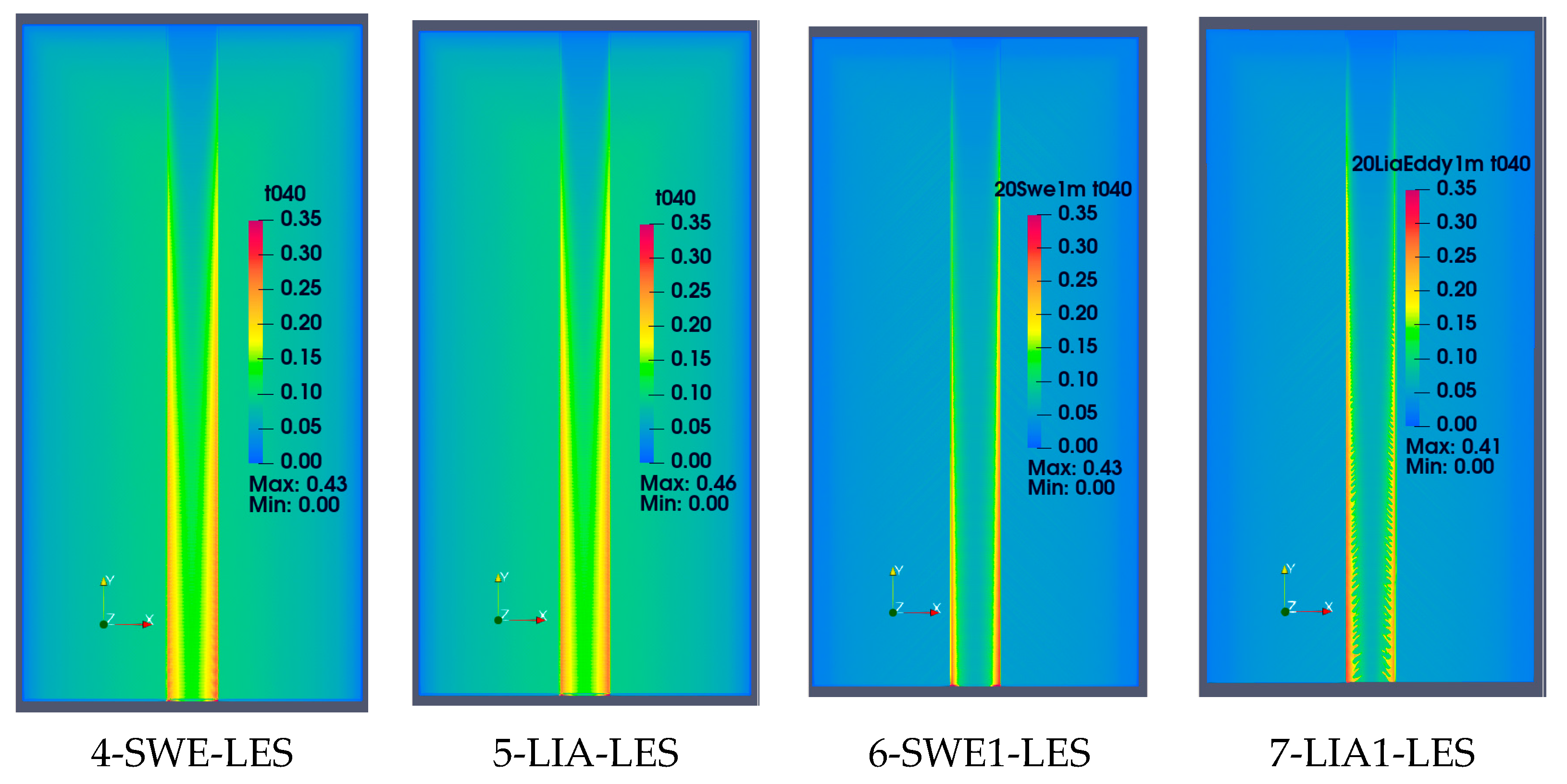
4.2.2. LES and Scale

The next set of contours describes water depths in W3 and the effects of Large Eddy Simulation or using a finer cell density (1 m × 1 m). Figure 9 illustrates several important and somewhat counter-intuitive results.

Figure 9 shows water depths at 40 min, past the peak rainfall intensity, but a location along the recession limb where the finer mesh solutions suffered instabilities. The most apparent difference results from the earlier peak flows from the fine mesh results and the much-reduced depth (more blue, less green). Figure 7c illustrates the same effect as a time series. The second significant difference appears in solution 7-LIA1-LES, where turbulence and instability occur along the break lines on the lower third of the watershed. Less noticeable turbulence is also evident along the 6-SWE1-LES solution. The instabilities may seem counter-intuitive for numerical models where typically a finer mesh results in reduced gradients and smoother results. However, for turbulent flow, this is not the case. As mentioned previously, overcomplexity can work against the numerical process.

4.2.3. Obstacles

The final set of contours involves flow between and around numerous obstacles, as presented in Figure 10. The most instructive conditions occur again in W3 (20%). Figure 10 presents the results for the final four solutions. Figure 10 shows the water depths at 64 min, below the recession curve’s inflection point. The color changes in the legend reflect the high percentage of shallow depths and emphasize the objects’ locations in the watershed. Note that all solutions have very deep water directly in front of the larger obstacles in the channel.

The slight difference in color over much of their regions indicates that the LIA solutions drain faster than SWEs. However, compared to Figure 9, turbulence does not appear along the break lines. The large obstructions slow the drainage process, precluding any highly turbulent activity along the longitudinal break lines that appeared before. While the cascading flow pattern is apparent, the solutions show slight instabilities (see also Figure 7c). The behavior near the center obstacles concentrates on (relatively) small zones. However, the maximum depths noted in the legends would indicate steep surface elevation gradients up against the obstacles. Recall that they were designated as weirs in the watershed layout, with heights that would not allow overtopping (even 3 m).

4.3. Froude Number Distribution

The Froude number indicates the subcritical (Fr < 1) or supercritical (Fr > 1) flow. The overland flow transitions further into supercritical as the watershed slope increases. On steep watersheds, the flow is predominantly supercritical. A high Froude number also signifies increased drag force, implying a higher rate of potential soil erosion [38]. This study placed obstructions along the watershed to encourage the subcritical flow and determine the transition zones between the sub- and supercritical flow. The obstructions can dissipate energy, as well.

The Froude number governs the drag force under laminar flow conditions (Reynolds number, Re < 500). Moreover, the hydraulic resistance in watersheds correlates more effectively with the Froude number [30]. Almeida and Bates [30] noted that the LIA solutions approximate the SWE more accurately with a Fr < 0.5, so knowing the location and extent of these zones will indicate the viability of LIA solutions. Previous studies [30] validated this approximation in open channel flow, while this study focused on sheet flow conditions. The Fr value is significant in this study for two reasons:

• Since low Fr numbers would only appear locally around obstructions, most flow is supercritical. The research above [30] stated that the LIA solutions work better in low Fr domains. However, their accuracy and stability remain uncertain under scattered sub- and supercritical conditions.
• Other studies have shown that the LIA solutions can produce an outflow time series similar to SWEs [40,41]. However, the Fr value plays a vital role in drag force and erosion. Analyses would require the Fr distribution throughout the watershed to understand drag force and erosion susceptibility better. With a detailed knowledge of the Fr distribution, the modeler could better examine the stability and accuracy of LIA solutions throughout the watershed (e.g., wave-like formations caused by the jumps from cell to cell).

The following figures are cropped, as shown in Figure 2 (red rectangle), to better display the details of distribution patterns. The center area represents the entire width of the flat central channel (150 m), while the side areas represent about one-third of each side slope’s total width (~125 m).

4.3.1. Basic

Figure 11 shows the Fr distribution in W1 for solutions 1-DWE, 2-SWE, and 3-LIA. The results of solution 1 differ significantly from those of 2 and 3. Solution 1 shows a value of Fr ~ 1.0 on the center channel, with side slopes of about Fr ~ 2.0. So, the flow is subcritical along the central channel but supercritical along the side slopes. Some color variations in all the solutions reflect the software’s choice to record maximum values over time, so the color shading shown may not occur at a single time step. Solutions 2 and 3 exhibit lower Fr values in the central channel and on both side slopes. Solution 2 has slightly higher Fr values in the center. Both solutions show oscillations on the side slopes above and below Fr = 1.0, as verified by the authors from magnified views, showing oscillation values below 1.0 (brownish-yellow) and above (yellow-orange with red streaks). Note that all of the oscillations appear normal to the direction of flow.

In Figure 12, the results change as the slope increases in W2. The Fr number increased in all the solutions, with supercritical flow on the side slopes and slightly subcritical flow in the center. Note the change in the Fr scale to a maximum value of 5.0; however, the color for Fr = 1.0 remains the same. The flow is so shallow in the dark red-brown areas that the solutions cannot calculate the Fr numbers.

In W3 (Figure 13), the solutions show similar characteristics. The black or brown side slopes indicate a shallow flow depth where the program cannot calculate the Fr. The middle areas show oscillations between subcritical and supercritical flow along the flow direction that indicate numerical errors. The similarities between results show that solutions 1 and 3 are similar along the central channel compared to solution 2. All the solutions struggle to calculate the Fr, especially on the left slope.

4.3.2. LES and Scale

In Figure 14, when LES is applied to W1, the shallow flow along the slopes becomes increasingly supercritical in solutions 4 and 5, with the middle area exhibiting more supercritical flow in solution 5. As the cell size reduces in solutions 6 and 7, the impact of the LES becomes more pronounced, resulting in the Fr values in solution 7 resembling those in solutions 4 and 6. In solution 7 (Figure 14), a wave-like periodic pattern in the Fr values appears, particularly along the sides. This pattern is likely a numerical artifact introduced by the LES component, causing the overland flow to resemble flow over weirs, with repeated fluctuations in the Fr values.

In W2, the LES impact is more pronounced, as shown in Figure 15. With solutions 4 and 5, some changes appear, mainly in solution 5, as the Fr numbers in the middle area approach the values of solution 4. However, the Fr distribution becomes similar if the cell size decreases in solutions 6 and 7. Even the values on the side slopes show more similarity with 1 × 1 cells. The side slopes in solutions 6 and 7 show numerical errors. The results show that the same cyclical errors appear on the sides, similar to W1, due to the LES in solutions 6 and 7. The visualization within the modeling software reaches its limits when the water depth becomes too shallow, although the surface oscillation appears in the calculation.

As the slope increased in W3 (Figure 16), the results showed similar problems as solution 5 (LIA+LES). The Fr distribution shows very little difference between W2 and W3. Although the Froude distribution is similar, the numerical errors on the outflow time series for solution 7 (Figure 6c) show that the solution is unusable.

The numerical error in the outflow time series shows that solution 7 is unusable. On the side slopes, the LES approach produced numerical errors. Besides these issues, grading the overall performance will be the benchmark for the problematic methods.

4.3.3. Obstructions

For W1, Figure 17 shows that the Froude distributions in solutions 8 and 10 (with LES) are similar, as are solutions 9 and 11. Since the LIA method does not include advection, the results indicate that applying LES does not cause solution 11 results to resemble those of solutions 8 or 10 more closely.

In W2, the Fr distributions exhibit a distinct pattern (Figure 18). The obstructions have a more significant impact here than in W1, resulting in higher Fr values both upstream and downstream of the obstruction. Solutions 8 and 10 produce similar results, with areas of lower Fr values closely adjacent to regions with higher Fr values. In contrast, solution 9 shows narrower bands of low Fr values, with values increasing further downstream from the obstructions. Solution 11 differs from all other solutions, displaying uniformly lower Fr values, indicating reduced drag force. Although the distribution pattern in solution 11 resembles that of solution 9, the Fr values are consistently lower.

The results for W3 (Figure 19) are similar to those observed for W1. The inclusion of LES does not affect the flow; solutions 8–10 and 9–11 are similar. The results are somewhat unexpected since the minor obstructions on both side slopes no longer show much influence. The reduced water depth and less reliable calculations may explain some differences.

As the slope increases, the Froude number also rises across the watershed, diminishing the obstruction’s impact on the Fr distribution in the central section. Upstream of the obstruction is a narrow zone of subcritical flow, while downstream, the area of shallow flow becomes more extended with increasing slope (from W1 to W3). In the middle of the watershed downstream of the obstructions and along the side slopes, the shallow depth—indicated by brown coloring—prevents accurate Fr calculation. Solution 11’s Fr values were also expected to show more significant variation in W3. Finally, the steeper slopes produced large areas where the calculation of the Fr became very problematic.

4.4. Reynolds Number Distribution

In evaluating the Reynolds (Re) number distribution, the goal was to find patterns in how the different solvers behave compared to each other. The following figures represent cropped parts of the solution (Figure 3) to show a more detailed representation of the results.

4.4.1. Basic

Figure 20, Figure 21 and Figure 22 illustrate the distributions of Reynolds numbers across watershed W1, W2, and W3. The overland flow depth decreases as the slope increases, often resulting in laminar flow with Reynolds numbers below 500. The simulations in this study showed that low Re occurs only on the side slopes, where the break-line effect is weak. In Figure 20, the side slopes show a wide range along with the center channel. Around break lines—where the slope changes—the Re value rises sharply due to the steeper gradient. This increase in Re becomes especially pronounced later around obstructions.

For watershed W1, the results from solutions 1, 2, and 3 align with expectations based on the differences among the solvers. The primary variation appears in the middle section of the watershed, where 1 and 2 differ the most, while 3 produces intermediate results. On the side slopes, shallow flow generates consistently low Re across all solutions. Re values increase sharply during the transition between the side slopes and the central flat slope, with this impact intensifying downstream.

In solution 1, this rapid increase in Re is followed by a gradual decrease, resulting in a narrow central section with lower Re values. However, solution 2 (SWE) shows higher turbulence over a broader range near the break line, with a more rapid reduction in Re values beyond this region. Also, as the slope increases, the backwater effect of the break lines on the side slope decreases. Therefore, as the slope increases, lower Re numbers would appear. As formerly mentioned, if the water depth is small, the software visualization reaches its limits. However, the small Re values also appeared in the calculation, so laminar (Re < 500) flow may have occurred in the shallow-depth regions.

In W2, the Reynolds numbers are lower on the side slopes than in W1 (Figure 21). Although the change in Re near the break line is still rapid, it is less intense, and the subsequent reduction occurs more quickly. The central middle section of W2 shows higher Re values than in W1, with a more uniform decrease in Re from upstream to downstream. Solution 3’s results remain intermediate, between solutions 1 and 2, but as the slope increases, the values and distribution resemble those of solution 2 more closely.

In W3 (Figure 22), solutions 2 and 3 show a similar pattern to that observed in W1 and W2: the Reynolds values decrease along the side slopes, and while Re increases near the break line, the rise is less intense, and the subsequent reduction occurs even more rapidly. Solution 1, however, displays a different pattern, with high Re values forming across a wider band around the break lines.

The basis for comparisons came from the results of the SWE solutions. The more turbulent behavior along the break lines agrees with expectations. The results from solution 1 showed significant differences caused by the lack of advection and turbulence terms in the DWE solution. While the 3-LIA solution showed similarities with solution 2-SWE, it also neglects advection.

4.4.2. LES and Scale

In W1, adding LES widens the highly turbulent paths, though the Re values decrease along the break lines. For a finer grid, the differences become more pronounced in solutions 6 and 7 (Figure 23). The Re values along the sides are smaller for finer grids, and the reduction is more gradual in the center, barely reaching the previous low Re numbers. Figure 23 displays the side slopes over a wide distance due to the break lines backwater effect, which causes low Re values only on the upper area of the side slopes. Due to the already low Re values, the LES component has minimal impact on the purely overland areas.

In W2 (Figure 24), the differences become more recognizable when the mesh’s resolution is higher (solutions 6 and 7). While solutions 4 and 5 are similar to solutions 2 and 3, solutions 6 and 7 differ. The Re number at the border rapidly decreases, but the Re number at the center of the middle watershed is lower than in solutions 4 and 5. The LES inclusion impact on the simulation is higher in the smaller cells. With smaller cells, higher Re values appeared on the side slopes.

In W3 (Figure 25), the results are similar to W2, although solution 7 differs more from the other results. The difference appears around the break lines. The Re values should be lower for a higher slope in the middle path, and the higher values should appear only on a narrow path near the break lines.

In W3, solutions 4 and 5 show a similar pattern to that observed in solutions 2 and 3. Including the LES did not have a significant impact. In solutions 6 and 7, the Re increases near the break line, with an intense rise, and the subsequent reduction occurs more rapidly. The final Re number is less in the middle than solutions 4 and 5; the flow is more laminar in the center.

4.4.3. Obstacles

In solutions 8, 9, 10, and 11 in W1 (Figure 26), obstructions produced higher turbulence, as expected. The Re value distribution reflected the shape of the Fr values, with the highest turbulence appearing in the central section as the flow exits the obstructions. Smaller Re peaks occurred where the obstructions and the break lines meet. Solutions 8 through 10 show only minor differences, with similar Re values across each solution. Variations occur primarily on the upstream side of the small walls and the side slopes, particularly where the walls intersect with the break lines. This effect is more pronounced in solutions 8 and 10, and LES did not impact these solutions significantly.

In W2 (Figure 27), the behavior changes. The Re number remains higher in the center downstream to the obstruction, but the high turbulence decreases faster on both sides. The small local turbulences upstream of the walls around the break lines disappear in solution 10. This turbulence could be an unwanted effect of the LES. The differences are minor between 9 and 11.

In W3 (Figure 28), all the solutions show visually similar Reynolds distributions. As the slope increases, the LES has a more reduced effect on the distribution of Re. The steeper slopes also generate shallower depths on the side slopes, with the accompanying loss of numerical accuracy in computing the Re.

During sheet flow conditions, the Froude number relates to the current discharge [38]. In this study, the land cover was homogenous, and the Froude number represented the governing coefficient quantifying the drag force on the flow [38]. The solutions performed more consistently with obstructions than without obstructions. While many solutions showed perturbations in flow, the obstructions moderated the flow so that numerical errors did not oscillate wildly. In cases without obstructions, solutions predicted flow accurately or diverged radically from expected behavior.

5. Discussion

Outflow Time Series, Peak Flows, and Volume Errors

Several different parameters can quantify how closely the solutions agree. Since no measured data applies to the hypothetical watersheds, computed outflow time series are compared. The SWE solution provided a baseline for comparison to the other solutions. The SWE solution for the obstacle watershed again provided a baseline for the obstacle group.

The flow data used for comparison consisted of outflow vs. time, peak flow, and volume. The flow data comparison used Nash–Sutcliff (NSE), Kling–Gupta (KGE), and Pearson correlation (γ_xy) formulas, where the SWE data was substituted for observed or measured data. So, the three formulas became

$$NSE=1-{\displaystyle \frac{{\sum }_{t=1}^T{\left(Q_B^t-Q_S^t\right)}^2}{{\sum }_{t=1}^T{\left(Q_B^t-{\overline{Q}}_S\right)}^2}}$$

(10)

$$KGE=1-\sqrt{{\left(r-1\right)}^2+{\left(\beta -1\right)}^2+{\left(\gamma -1\right)}^2}$$

(11)

$$\beta ={\displaystyle \frac{{\mu }_S}{{\mu }_B}}\gamma ={\displaystyle \frac{{CV}_S}{{CV}_B}}={\displaystyle \frac{{\sigma }_S/{\mu }_S}{{\sigma }_B/{\mu }_B}}$$

where KGE is the Kling–Gupta Error statistic, r is the correlation coefficient between the baseline and solver runoff values, β is the bias ratio, γ is the variability ratio, μ is the mean runoff, CV is the coefficient of variation, σ is the standard deviation of runoff, and the indices S and B represent the solution and baseline runoff values, respectively. Finally, the Pearson correlation coefficient γ_xy resulted from

$${\gamma }_{xy}={\displaystyle \frac{{\sum }_{t=1}^T\left(Q_B^t-{\overline{Q}}_B\right)\left(Q_S^t-{\overline{Q}}_S\right)}{\sqrt{{\sum }_{t=1}^T{\left(Q_B^t-{\overline{Q}}_B\right)}^2}\sqrt{{\sum }_{t=1}^T{\left(Q_S^t-{\overline{Q}}_S\right)}^2}}}$$

(12)

where Equation (7) describes the time series flow values.

Table 2. Error and correlation coefficients for various solutions compared to SWE baseline.

		W-1 5%			W-2 10%			W-3 20%
Base	Compare	NSE	KGE	Pearson	NSE	KGE	Pearson	NSE	KGE	Pearson
2-Swe	1-Diff	0.994	0.987	0.997	0.995	0.958	0.998	0.665	0.760	0.817
2-Swe	3-Lia	0.994	0.986	0.997	0.995	0.954	0.998	0.971	0.926	0.987
2-Swe	4-Swe-Les	0.994	0.987	1.000	1.000	1.000	1.000	1.000	1.000	1.000
2-Swe	5-Lia-Les	0.995	0.987	1.000	0.995	0.956	0.998	0.969	0.911	0.987
2-Swe	6-Swe1-Les	0.978	0.922	1.000	0.938	0.885	1.000	0.881	0.862	0.999
2-Swe	7-Lia1-Les	0.979	0.962	1.000	0.953	0.890	0.998	0.862	0.820	0.987
8-SweO	9-LiaO	0.990	0.942	0.996	0.970	0.919	0.987	0.923	0.892	0.963
8-SweO	10-SweO-Les	1.000	1.000	1.000	1.000	1.000	1.000	1.000	1.000	1.000
8-SweO	11-LiaO-Les	0.993	1.000	0.998	0.978	1.000	0.991	0.973	1.000	0.988

Green = Basic scenarios, Orange = LES and Scale, Blue = Obstacles.

lists all the comparisons. Note that the most apparent deviations are associated with the diffuse equation in watershed W3, with slopes of 20% (italics, row 1). Perhaps more surprising are the correlations between the 1 m × 1 m mesh and the baseline 2 m × 2 m (italics rows 5,6). An examination of the hydrographs supports these values.

The results show minor differences. However, these values represent the outflow time series. Therefore, fast, simplified solvers could represent less detailed hydrodynamical watershed models. On the other hand, both NSME and KGE values for model 1 do not differ, although some of the time series were problematic. So, the values from Table 2 mean that for detailed overland hydrodynamical models, the NSE and KGE values and volume differences do not represent the areal accuracy of a 2D model.

The final comparison parameter was the overall numerical volume error from the lossless overland and peak flow (

Table 3. Summary of peak flows and overall volume errors for each solution.

	W1		W2		W3
Solution	Qmax [cms]	Verror [%]	Qmax [cms]	Verror [%]	Qmax [cms]	Verror [%]
1-DWE	46.15	0.03	47.92	0.04	145.51	0.02
2-SWE	47.25	0.03	46.99	0.28	46.88	0.16
3-LIA	46.16	0.03	48.06	0.37	49.34	0.15
4-SWE+LES	46.17	0.03	46.97	0.28	47.14	0.05
5-LIA+LES	46.20	0.03	47.78	0.36	51.84	0.12
6-SWE1+LES	47.92	0.03	51.52	0.13	51.57	0.61
7-LIA1+LES	46.45	0.03	51.04	0.18	57.32	0.39
8-SWEO	34.11	0.06	41.38	0.75	45.32	0.80
9-LIAO	37.46	0.02	45.62	0.03	51.54	0.10
10-SWEO+LES	34.10	0.07	41.37	0.76	45.35	0.79
11-LIAO+LES	36.90	0.02	44.94	0.03	48.92	0.17

Green = Basic scenarios, Orange = LES and Scale, Blue = Obstacles.

). It is important to note that in this comparison, the emphasis is not on the error magnitude but on the differences and ratios relative to the other solutions. The overall volume error was generally low due to the stability of most solutions and simplified geometry. Note, however, that even with 4% of the overall volume error, the HEC-RAS model sends warnings to the simulation log file. For watershed W1, all solutions produce consistent results for Q_max and V_error. The impact of obstacles reducing peak flows is apparent within W1, with a nearly 25% reduction in Q_max. For W2, Q_max shows more variability among solutions, especially with the 1 m × 1 m mesh (italics row 7). V_error varies over a broader range, as well, but within reasonable limits. The obstacles also reduce peak flow in this watershed, but not as much. The most notable errors appear in W3 with the DWE solution due to instability (italics, row 1). The other solutions show wider variations in W3 compared to W1 and W2, highlighting the increased computational difficulties that arise along steeper slopes.

The variation in peak flows, with or without obstructions, was minimal. Previous studies [25] suggested that more straightforward methods might underestimate peak flows; however, this study found no significant differences, even when using the DWE method (except in cases of instability, indicated in italics).

Volume errors were generally consistent with observations from other studies [30]: as solution complexity increased, so did volume errors, even when solution stability was maintained. For watersheds W2 and W3, the Local Inertia Approximation (LIA) generated the highest error, with no improvement observed from adding LES. A finer grid reduced the volume error in W2 but increased it in W3. The most significant numerical error was observed in W3 with the SWE and LES on a finer grid [italics, rows 6,7).

These simulations aimed to highlight the errors produced solely by different solver methods. These errors were sometimes minor, primarily because solution stability was carefully maintained. The mesh distribution remained consistent and refined enough to accurately capture overland flow velocities at the given time steps. During simulations, time steps satisfied the Courant ratio, and the watershed geometry was simplified, including slight but necessary adjustments with and without distributed obstructions to simulate basic turbulent flow states. The outflow boundary condition and rainfall model were also simplified, with precipitation applied uniformly across the watershed and distributed linearly over time. These controlled conditions were essential to closely simulate the behavior of a natural watershed while avoiding instabilities related to geometry. Consequently, the comparison could focus specifically on numerical errors arising from the different solvers.

Two workstations performed analyses: an Intel i9-13900KS and a dual AMD Epyc 7B12. The analyses utilized 100% of the available cores to compute the unsteady flow problem. An SSD drive stored all the data files. One comprehensive project file contained the entire analysis suite with many subfolders corresponding to the conditions listed in Table 1 and watersheds W1, W2, and W3 for 33 plans. The typical analysis times lasted about 1 h.

Table 4. Comparison of solution times for equation models and watersheds.

Model	W1			W2			W3
	Sim/SWE Ratio	Avg Time Step [s]	Sim/Event Ratio	Sim/SWE Ratio	Avg Time Step [s]	Sim/Event Ratio	Sim/SWE Ratio	Avg Time Step [s]	Sim/Event Ratio
1	0.6	0.4	8	0.6	0.4	7.76	0.4	0.4	4.14
2	1.0	0.4	4.87	1.0	0.4	4.29	1.0	0.3	2.25
3	0.8	0.4	6.08	0.8	0.4	5.2	1.0	0.4	2.23
4	1.2	0.4	4.2	1.2	0.4	3.71	0.9	0.3	2.41
5	1.1	0.4	4.3	1.1	0.4	3.83	1.1	0.4	2.01
6	5.0	0.4	0.98	6.4	0.3	0.67	6.1	0.2	0.37
7	5.0	0.4	0.98	6.4	0.3	0.67	6.0	0.2	0.38
8	1.0	0.4	4.66	1.0	0.3	2.53	1.0	0.2	2.06
9	1.3	0.3	3.66	0.7	0.3	3.65	1.0	0.2	2.12
10	1.2	0.4	4	1.1	0.3	2.21	1.1	0.2	1.81
11	1.8	0.3	2.59	1.0	0.3	2.56	1.0	0.3	1.97

Green = Basic scenarios, Orange = LES and Scale, Blue = Obstacles.

illustrates the execution times for the various solution conditions. In order to compare solution methods, the 2-SWE solution provides a baseline for normalizing as a solution time ratio, where

$$Solution Ratio={\displaystyle \frac{{Time}_i}{{Time}_{SWE}}}$$

(13)

and, comparing the numerical solution time to the event time (180 min for all events and solutions), results in a simulation-to-event ratio where

$${\displaystyle \frac{Sim}{Event}}={\displaystyle \frac{\left(Simulation Compute Time\right)}{180 minutes}}$$

(14)

Table 4 compares solution times for the various solutions attempted. The computational details showed that the DWE method is the fastest. Although the LIA method’s complexity is between the DWE and SWE solver, the difference in computation time is not significantly faster compared to the SWE solver. The computation can execute slower, even with the LES feature. The maximum time step was limited to 0.4 s to guarantee stability.

Various refinements explored the effects of more restrictive computational tolerances for surface water elevations and cell volumes. They produced slightly better results; however, the earlier instabilities persisted, and compute times often increased to 12 h for a single event.

When the watershed slopes increased, the effect of the LIA model’s simplification started to appear, with the average time step remaining stable at steeper slopes. This difference correlates with the HEC-RAS manual: the LIA method can grant around 30% more stability. Another significant finding demonstrated that increasing the mesh resolution will not improve the models’ accuracy, although the simulation time becomes significantly slower in models 6 and 7. The possible overcomplexity of the SWE+LES method was not an issue, but recall that the geometries were simplified. These issues can quickly appear in a natural watershed. Perhaps with SWE+LES simulations, the model may become more stable, but the overall runtime and internal oscillation errors may increase.

The maximum time step where no additional iterations appear depends on the model’s geometry and mesh size. The SWE-based simulations were sensitive along the break lines, where even the shortest time step, 0.025 s, could not produce stability. The LIA+LES method had fewer stability issues [30].

6. Conclusions

Flow calculations are often unstable in natural, steep-sloped watersheds with creek beds, abrupt slope changes, and random obstructions, leading to volume errors or inconsistencies in the outflow time series. Such errors can manifest as oscillations or sudden jumps in time series data—numerical artifacts that do not always appear in the overall volume error. Additionally, with complex geometries, certain advanced methods may cause solution crashes during simulation [42]. More straightforward but comparably effective solvers, enhanced with LES components, may provide a more reliable approach.

This study compared only the numerical errors arising from overland flow. A comprehensive flash flood model, however, requires additional elements, including the following:

• Infiltration Losses: depend on the infiltration model and are linked to the mesh.
• Additional Losses: canopy interception, forest floor debris [42], and other localized features may disrupt surface flow processes in the watershed.
• Effects of Structures: culverts, bridges, and natural obstructions in the creek bed or watershed can significantly alter turbulent flow.
• Higher Depth and Flow Rates: when flow rates increase they may introduce further volume errors as flow behavior changes [43].
• Variability in Rainfall Events: modeling actual rainfall events introduces changes in incoming flow, which can lead to local instabilities.

Besides simulating flow dynamics, other elements contribute to their errors, which can compound the total solution error. For ungauged watersheds, it is imperative to minimize numerical errors to improve calculation accuracy and prevent unnecessary errors. Each investigated parameter served to measure the effectiveness of each solver:

• Outflow Time Series: a comparison of the peak timing and peak flow and the identification of numerical errors that may appear in the rising and falling limbs.
• Distribution of Hydraulic Depth: Mapping the water depths over time highlighted the changing distribution of water throughout the watershed. The locations where instabilities may occur became evident. The impact of obstructions on overall flow patterns also became more apparent.
• Froude Number: Useful in overland flow, mainly where supercritical flow and minor turbulence occur. The Froude number reflected drag force, indicating potential erosion.
• Reynolds Number: Critical in sheet flow where values should ideally be Re < 500 in plains. Turbulence around creek beds and obstructions is also important to capture.
• Overall Volume Error: Summarizes errors from each solver method, ideally minimized. According to the HEC-RAS manual [source], the simulation logs warn if the volume error exceeds 4%. In ungauged watersheds, added model components can quickly increase these errors.

Notably, most errors appeared in W3, which has the steepest slope (although some unexpected errors appeared only in W2). These results suggest that slope steepness contributes to error patterns, as well as specific watershed features. In W3, obstructions helped correct some initial errors, though they introduced a trade-off with increased volume error due to the added complexity of turbulent flow calculations.

The Diffusion Wave Equation (DWE) method proved unsuitable for steep slopes, lacking the capability to capture turbulent flow behavior accurately. While commonly used for large-scale hydrological models with simplified geometries, the DWE method’s oversimplification limits its applicability for flash-flood modeling in detailed, small-scale watersheds. Additionally, the lack of advection and inability to add an LES component made this solver unsuitable for detailed, highly turbulent flows.

The Shallow Water Equation (SWE) model served as the baseline for comparison due to its comprehensive handling of flow dynamics. For largely ungauged watersheds, the SWE generated accurate flow simulations. However, the SWE is highly sensitive to mesh geometry, which can lead to additional volume error from iterative calculations, even if the model remains stable. For models where accurate flow behavior within the watershed is a priority, this volume error can be considered acceptable as long as peak flow errors remain within reasonable bounds.

The Local Inertia Approximation (LIA) model demonstrated strong performance, especially in high-slope, uncomplicated terrains. In these cases, LIA effectively estimates SWE results with less sensitivity to geometry, making it a practical option when watershed conditions support its simplifications.

Adding the Large Eddy Simulation (LES) component can enhance or hinder a model’s accuracy, depending on the chosen solver and watershed conditions. With the SWE method, LES sometimes exacerbated volume errors and introduced hidden instabilities. However, for the LIA model, the LES addition was generally beneficial, improving the model’s capacity to approximate turbulent behavior around obstructions and in time series. Caution is advised, though, as this pairing performed less effectively in W2 for the Froude number distribution. A preliminary comparison between the LIA + LES combination and the SWE model in a simplified setting is recommended before deploying it in project-specific applications to maximize reliability.

As the slopes increase, the flow is more driven by the effect of gravity. Therefore, the SWE method could have stability issues because advection drives its calculation. However, the results of the simulations were consistent with each other. With an increased slope, the LES option could cause complications with the LIA model. On the other hand, when obstructions appear, the SWE method’s complexity represents the turbulent flow well at the cost of sensitivity to the sudden changes in the slope. The results have shown that despite the increasing Froude numbers, the results of the LIA methods did not diverge from the SWE results. As the Reynolds value distribution showed, the simplified LIA method with the additional LES gives proper results. The differences between the results were minor, even with an increased slope. Also, the LIA method’s visual representation of the overland, shallow flow is better when the slopes become steeper.

Simulating rainfall-induced overland flow in small, steep, and often ungauged watersheds is inherently challenging. Depth-integrated models, such as those in this study, offer practical solutions but demand careful consideration of each solver’s strengths and limitations. The findings affirm that each solver method has advantages depending on the scenario and that understanding their specific behaviors under different conditions is essential, rather than disregarding any solver entirely. These findings become especially relevant in ungauged watersheds, where high uncertainty underscores the need for precise model selection and calibration.

References

- Brunner, G. HEC-RAS, River Analysis System Hydraulic Reference Manual (Ver. 6.6). 2024. Available online: https://www.hec.usace.army.mil/confluence/rasdocs/ras1dtechref/latest (accessed on 12 March 2025).
- Garambois, P.A.; Larnier, K.; Roux, H.; Labat, D.; Dartus, D. Analysis of flash flood-triggering rainfall for a process-oriented hydrological model. Atmos. Res. 2014, 137, 14–24. [Google Scholar] [CrossRef]
- Blöschl, G.; Sivapalan, M.; Wagener, T.; Viglione, A.; Savenije, H. A data acquisition framework for predictions of runoff in ungauged basins. In Runoff Prediction in Ungauged Basins, Synthesis Across Processes, Places and Scales; Cambridge University Press: Cambridge, UK, 2013. [Google Scholar]
- Huang, W.; Cao, Z.; Huang, M.; Duan, W.; Ni, Y.; Yang, W. A New Flash Flood Warning Scheme Based on Hydrodynam-ic Modelling. Water 2019, 11, 1221. [Google Scholar] [CrossRef]
- Wu, W.; Shields, F.D.; Bennet, S.; Wang, S.S.Y. A depth-averaged two-dimensional model for flow, sediment transport, and bed btopography in curved channels with riparian vegetation. Water Resour. Res. 2005, 41, W03015. [Google Scholar] [CrossRef]
- Huang, W.; Cao, Z.; Qi, W.; Pender, G.; Zhao, K. Full 2D Hydrodynamic Modelling of Rainfall-induced Flash Floods. J. Mt. Sci. 2015, 12, 1203–1218. [Google Scholar] [CrossRef]
- Costabile, P.; Costanzo, C.; Ferraro, D.; Macchiona, F.; Petaccia, G. Performance of the New HEC-RAS Version 5 for 2-D Hydrodynamic-Based Rainfall-Runoff Simulations at Basin Scale: Comparison with a State-of-the Art Model. Water 2020, 12, 2326. [Google Scholar] [CrossRef]
- Ion, S.; Marinescu, D.; Cruceanu, S. Riemann Problem for Shallow Water Equation with Vegetation. An. St. Univ. Ovidius Constanta 2018, 26, 145–173. [Google Scholar] [CrossRef]
- Hromadka, T.V.; Rao, P. Application of Diffusion Hydrodynamic Model for Overland Flows. Open J. Fluid Dyn. 2019, 9, 334–345. [Google Scholar] [CrossRef]
- Mihu-Pintilie, A.; Cimpianu, C.I.; Stoleriu, C.C.; Pérez, M.N.; Paveluc, L.E. Using High-Density LiDAR Data and 2D Streamflow Hydraulic Modeling to Improve Urban Flood Hazard Maps: A HEC-RAS Multi-Scenario Approach. Water 2019, 11, 1832. [Google Scholar] [CrossRef]
- Rana, V.K.; Suryanarayana, T.M.V. Estimation of flood influencing characteristics of watershed and their impact on flooding in data-scarce region. Ann. Gis 2021, 27, 397–418. [Google Scholar] [CrossRef]
- Zhao, J.; Liang, Q. Novel variable reconstruction and friction term discretisation schemes for hydrodynamic model-ling of overland flow and surface water flooding. Adv. Water Resour. 2022, 163, 104187. [Google Scholar] [CrossRef]
- Costabile, P.; Constanzo, C.; Macchione, F. Numerical aspects in simulating overland flow events. In Proceedings of the First IAHR European Congress, Edinburgh, UK, 4–6 May 2010. [Google Scholar]
- Pokrajac, D. Depth-integrated Reynolds-averaged Navier–Stokes equations for shallow flows over rough permeable beds. J. Hydraul. Res. 2013, 51, 597–600. [Google Scholar] [CrossRef]
- Costabile, P.; Costanzo, C.; Macchione, F.; Mercogliano, P. Two-dimensional model for overland flow simulations: A case study. Eur. Water 2012, 38, 13–23. [Google Scholar]
- Ámon, G.; Bene, K. Impact of different rainfall events on overland flow using a 2D hydrodynamical model on a steep-sloped watershed. In Proceedings of the EGU General Assembly 2023, Vienna, Austria, 24–28 April 2023. EGU23-9179. [Google Scholar] [CrossRef]
- Garcia-Lovella, Y.; Moya, I.H.; Rubio-Rodriguez, M.A.; Jayasuriya, J. Assessment of LES Dynamic Smagorinsky-Lilly model resolution for combustion engineering applications. DYNA 2023, 90, 95–104. [Google Scholar]
- Mehta, D.; Zhang, Y.; Van Zuijlen, A.; Bijl, H. Large Eddy Simulation with Energy-Conserving Schemes and the Sma-gorinsky Model: A Note on Accuracy and Computational Efficiency. Energies 2019, 12, 129. [Google Scholar] [CrossRef]
- Laurila, E.; Roenby, J.; Maakala, V.; Peltonen, P.; Kahila, H.; Vuorinen, V. Analysis of viscous fluid flow in a pressure-swirl atomizer using large-eddy simulation. Int. J. Multiph. Flow 2019, 113, 371–388. [Google Scholar]
- Jourabian, M.; Armenio, V. Large Eddy Simulation (LES) of Suspended Sediment Transport (SST) at a Laboratory Scale. In Proceedings of the 26th International Ocean and Polar Engineering Conference, Rhodes, Greece, 26 June–21 July 2016. [Google Scholar]
- Almeida, G.A.M.; Bates, P.; Freer, J.E.; Souvignet, M. Improving the stability of a simple formulation of the shallow water equations for 2-D flood modeling. Water Resour. Res. 2012, 48, W05528. [Google Scholar] [CrossRef]
- Martins, R.; Leandro, J.; Chen, A.S.; Djordevic, S. A comparison of three dual drainage models: Shallow water vs local inertial vs diffusive wave. J. Hydroinform. 2017, 19, jh2017075. [Google Scholar] [CrossRef]
- Costabile, P.; Costanzo, C.; Macchione, F. Comparative analysis of overland flow models using finite volume schemes. J. Hydroinform. 2012, 14, 122–135. [Google Scholar] [CrossRef]
- Ogden, F.L.; Julien, P.Y. Runoff Sensitivity to Temporal and Spatial Rainfall Variability at Runoff Plate and Small Basin Scale. Water Resour. Res. 1993, 29, 2589–2597. [Google Scholar]
- Xia, X.; Liang, Q.; Ming, X.; Hou, J. An efficient and stable hydrodynamic model with novel source term discretization schemes for overland flow and flood simulations. Water Resour. Res. 2017, 53, 3730–3759. [Google Scholar] [CrossRef]
- Sanchez, A. Advanced Parameters in HEC-RAS. 2022. Available online: https://www.hec.usace.army.mil/confluence/prospect/files/179605245/179605315/2/1711746389465/2.8+Advanced+Computation+Options.pdf (accessed on 14 January 2025).
- Sanchez, A. HEC-RAS 2D Turbulence Models: Approach, Equations, Coefficients. 2022. Available online: https://www.youtube.com/watch?v=ePVdhuwCpmQ (accessed on 22 January 2025).
- Ballesteros-Cánovas, J.A.; Galán, M.Á.E.; Bodoque, J.M.; Díez-Herrero, A.; Stoffel, M.; Gutiérrez-Pérez, I. Estimating flash flood discharge in an ungauged mountain catchment with 2D hydraulic models and dendrogeomorphic palaeostage indicators. Hydrol. Process. 2011, 25, 970–979. [Google Scholar]
- Paraview Users Guide Version 5.10.0. 2025. Available online: https://docs.paraview.org/en/latest/UsersGuide/index.html (accessed on 10 March 2025).
- Almeida, G.A.M.; Bates, P. Applicability of the local inertial approximation of the shallow water equations to flood modeling. Water Resour. Res. 2013, 49, 4833–4844. [Google Scholar] [CrossRef]
- Isaev, S.A.; Kornev, N.V.; Leontiev, A.I.; Hassel, E. Influence of the Reynolds number and the spherical dimple depth on turbulent heat transfer and hydraulic loss in a narrow channel. Int. J. Heat Mass Transf. 2010, 53, 178–197. [Google Scholar]
- Li, P.; Zhang, K.; Wang, J.; Meng, H.; Nicosia, A.; Ferro, V. Overland flow hydrodynamic characteristics in rough beds at low Reynolds numbers. J. Hydrol. 2022, 607, 127555. [Google Scholar]
- Ferro, V.; Guida, G. A theoretically-based overland flow resistance law for upland grassland habitats. Catena 2022, 210, 105863. [Google Scholar]
- Stamou, A.I.; Papadonikolaki, G.; Gkesouli, A.; Nikoletopoulos, A. Modeling the effect of vegetation on river flood-plain hydraulics. Glob. NEST J. 2012, 14, 371–377. [Google Scholar]
- Zhang, H.; Wang, Z.; Dai, L.; Xu, W. Influence of Vegetation on Turbulence Characteristics and Reynolds Shear Stress in Partly Vegetated Channel. J. Fluids Eng. 2015, 137, 061201. [Google Scholar] [CrossRef]
- Hardy, R.J.; Best, J.L.; Lane, S.N.; Carbonneau, P.E. Coherent flow structures in a depth-limited flow over a gravel surface: The role of near-bed turbulence and influence of Reynolds number. J. Geophys. Res. 2010, 114, F01003. [Google Scholar] [CrossRef]
- Rousseau, M.; Cerdan, O.; Delestre, O.; Dupros, F.; James, F.; Cordier, S. Overland Flow Modelling with the Shallow Water Equation Using a Well Balanced Numerical Scheme: Adding Efficiency or just More Complexity? 2012. Available online: https://hal.archives-ouvertes.fr/hal-00664535/ (accessed on 12 January 2025).
- Cantalice, J.; Dias, I.C.G.M.; Andrade, D.S.; Filho, F.M.A.; Souza, W.; Nunes, E.O.S.; Guerra, S.M.S.; Paula Silva, V.; Sartori, L.; Freitas, F.J.; et al. Hydraulic resistance to overland flow governed by Froude number on semi-arid hillslopes under shrubs and crops. Hydrol. Sci. J. 2021, 66, 1531–1540. [Google Scholar] [CrossRef]
- HDFView (Ver 3.3.2) User Manual. Available online: https://www.hdfgroup.org/download-hdfview/ (accessed on 10 March 2025).
- Chang, Y.S.; Scotti, A. Modeling unsteady turbulent flows over ripples: Reynolds-averaged Navier-Stokes equations (RANS) versus large-eddy simulation (LES). J. Geophys. Res. 2004, 109, C09012. [Google Scholar] [CrossRef]
- Lago, C.A.F.; Giacomoni, M.; Bentivoglio, R.; Taormina, R.; Gomes, M.N.; Mendiondo, E.M. Generalizing rapid flood predictions to unseen urban catchments with conditional generative adversarial networks. J. Hydrol. 2023, 618, 129276. [Google Scholar] [CrossRef]
- Ámon, G.; Bene, K. Importance of Eddy Viscosity and Advection in Hydrodynamical Models for Simulating Flash Floods on Steep Sloped Watersheds. Chem. Eng. Trans. 2024, 114, 805–810. [Google Scholar]
- Ámon, G.; Bene, K.; Ray, R.; Gribovszki, Z.; Kalicz, P. Improving Flash Flood Hydrodynamic Simulations by Inte-grating Leaf Litter and Interception Processes in Steep-Sloped Natural Watersheds. Water 2024, 16, 750. [Google Scholar] [CrossRef]