Article

Assessing the Effects of Bioenergy Cropping Scenarios on the Surface Water and Groundwater of an Intensively Agricultural Basin in Central Greece

by
Maria Sismanidi
1,
Lamprini Kokkinaki
1,
Sofia Kavalieratou
1,
Haralampos Georgoussis
1,
Kyriakos D. Giannoulis
2,
Elias Dimitriou
3 and
Yiannis Panagopoulos
1,*
1
Department of Hydraulics, Soil Science and Agricultural Engineering, School of Agriculture, Aristotle University of Thessaloniki, 54124 Thessaloniki, Greece
2
Laboratory of Agronomy and Applied Crop Physiology, Department of Agriculture, Crop Production & Rural Environment, University of Thessaly, Fytokoy Str., 38446 Volos, Greece
3
Hellenic Centre for Marine Research, Institute of Marine Biological Resources and Inland Waters, 46.7 km Athens—Sounio Ave., 19013 Anavyssos, Attica, Greece
*
Author to whom correspondence should be addressed.
Hydrology 2025, 12(4), 66; https://doi.org/10.3390/hydrology12040066
Submission received: 6 February 2025 / Revised: 19 March 2025 / Accepted: 20 March 2025 / Published: 22 March 2025

Abstract

Pinios river basin constitutes the most important agricultural production area in Greece but contributes to the degradation of the quality and quantity of surface water and groundwater bodies. Bioenergy crops implemented as part of the existing cropping systems could be a novel and efficient mitigation strategy against water degradation, contributing to the production of energy through renewable sources. This study uses the Soil and Water Assessment Tool (SWAT) to first develop a representative model of Pinios river basin and evaluate its current state with respect to water availability and nitrate water pollution. A low-input perennial bioenergy crop, switchgrass, is then simulated closely to the Greek conditions to investigate its potential effects on water in three implementation scenarios: the installation and growth of switchgrass in the entire irrigated cropland, exclusively in irrigated sloping (slopes > 1.5%) cropland, and exclusively in irrigated non-sloping cropland. The simulated results demonstrate that under all scenarios, the water quality improvements with respect to the nitrate loads entering surface water and groundwater bodies were significant, with their reduction being directly affected by the extent to which switchgrass replaced resource-demanding conventional crops. Specifically, the reduction in the annual nitrate loads in the surface water under these three scenarios varied from 7% to 18% at the river basin scale, while in certain cropland areas, the respective reduction even exceeded a level of 80%. The potential to improve the water status was also considerable, as the implementation of the bioenergy crop reduced the irrigation water used annually in the basin by 10% (64 Mm3) when switchgrass replaced the conventional crops only on the sloping land and by almost 30% (187 Mm3) when it replaced them throughout the irrigated land. At the same time, significant biomass production above 18 t/ha/y applied in all of the simulations. This study also highlights the contribution of the bioenergy crop to the rehabilitation of the groundwater levels across the basin, with the possibility of increasing them by >50% compared to the baseline, implying that the adoption of switchgrass could be a promising means against water scarcity.

1. Introduction

Water degradation is often caused by the intensification of agricultural activities. Especially around the rural landscape of the Mediterranean region, agriculture has led to the overexploitation of water reserves for irrigation and to a decline in water quality due to non-point source pollutants like fertilizers and pesticide residues entering water bodies [1,2,3,4,5]. While intensive agriculture is crucial for food, feed, and fiber production, achieving a balance between water quality and quantity is a challenge. Therefore, appropriate management practices are required to accomplish these conflicting objectives and meet the objective of a good ecological status required by the Water Framework Directive (WFD) (Directive 2000/60/EC, 2000) and the Nitrates Directive (Directive 91/676/EEC) [6].
In addition, agriculture is being promoted globally as a significant method for sustainable energy production through the cultivation of bioenergy crops for renewable energy. The European Union (EU) has implemented measures to advance biofuels through the Renewable Energy Directive (Directive 2018/2001), which is part of the European Green Deal aiming for a climate-neutral EU by 2050. Biomass and biofuels are seen as promising energy sources within the current energy crisis in the EU, as they can be produced domestically, thereby reducing the dependence on energy imports. The need to increase bioenergy production in Greece has been recognized in recent decades [7]. Efforts to increase the combined heat and power production from biomass and to replace portions of gasoline and diesel with liquid biofuel have been reported from more than a decade [8]. However, the national use of renewable energy sources remains low. As an EU member state, Greece must comply with the European Directive, which, for example, mandates that biofuels should contribute to >10% of the total transport energy consumption by 2030 [9].
Besides energy targets, bioenergy production can, however, have positive environmental impacts when it comes from bioenergy crops that are incorporated within existing resource-demanding cropping systems. Specifically, perennial bioenergy crops are considered a viable option since they have the capacity to substantially reduce nitrate losses and subsequently reduce non-point source pollution [10]. In addition, bioenergy crops like sunflower and sorghum require less irrigation water than most irrigated crops, enhancing groundwater conservation [11]. In particular, the perennial bioenergy crop switchgrass, introduced from the US and characterized as low-input, is expected to exhibit similar behavior. Nevertheless, producing bioenergy requires extensive agricultural areas, often leading to significant land use changes. Therefore, it is essential to assess a bioenergy crop’s socio-economic and environmental footprint before selecting it for regional planning. In Greece, no such plan has yet been proposed for any agricultural region to ensure the continuous, uninterrupted production of bioenergy products.
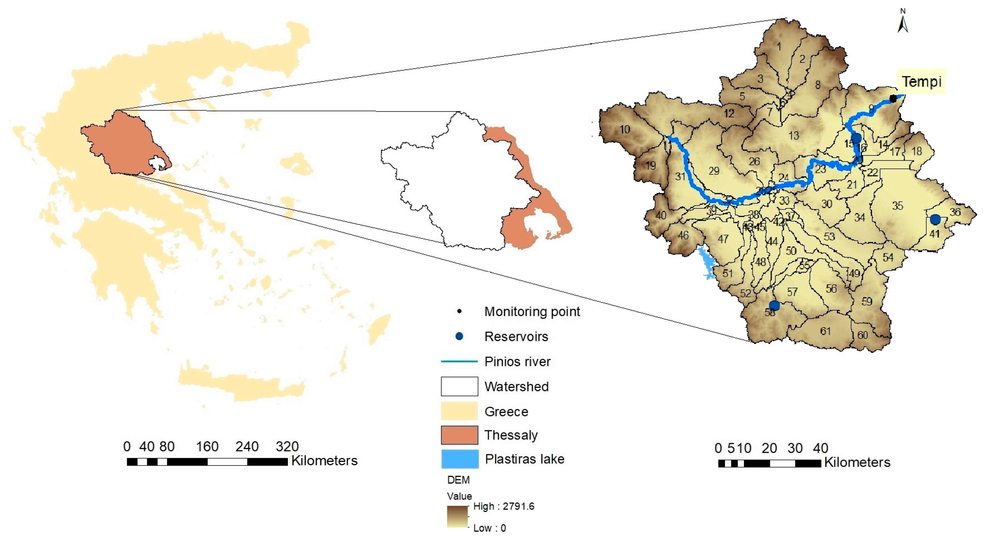
The Thessaly plain, located in the center of Greece, represents the most important agricultural producer in the country. The largest river basin in the area is Pinios river basin (PRB), covering roughly 11,000 km2. It is characterized by a Mediterranean climate, fertile soils, and a mild topography and is considered ideal for a variety of crop cultivation. These characteristics have caused the intensification of irrigated agriculture in the region, with water quantity and quality implications [5,12]. This region is included in the list of areas characterized as nitrate-vulnerable zones, with a negative water balance [13].
For the assessment of land use changes at the river basin scale, including changes in cropping patterns and their effects on water resources, advanced hydrological models that can provide time-efficient water quantity and quality predictions are widely utilized. Specifically, the process-based Soil and Water Assessment Tool (SWAT) model has been used worldwide in a wide range of studies, among which one can find a few involving bioenergy crop simulations [14,15,16]. Of substantial interest to the present paper are SWAT studies on bioenergy crops that have highlighted significant nitrate loss reductions and considerable biomass accumulation for potential energy production, even when they are grown in low-productivity areas [17,18]. Moreover, Gassman et al. [19] found that the realistic, limited inclusion of bioenergy crops within agricultural systems can result in a considerable reduction in the loss of nitrates from land to water.
Recent publications on SWAT from Greece that can be considered relevant to the present study are only studies that have investigated the impacts of water management practices on the hydrological status of rivers or the water budgets of agricultural areas, as well as studies that have dealt with land use changes and their effects on pollution loads [20,21,22]. To the best of our knowledge, no studies dealing with bioenergy crop simulation in Greece exist in the literature.
The present study aims to build a dynamic SWAT hydrological and management model of the intensively managed PRB that considers climate, land use, and agricultural practices to estimate the crop yields and evaluate the resulting quantity and quality of the surface water and groundwater. Using this model, this study is the first to attempt a realistic simulation of the switchgrass growth cycle in Greece and execute rough scenarios of its implementation across large agricultural areas in order to explore the potential upper levels of water improvements and biomass production at the river basin scale.

2. Materials and Methods

2.1. The Study Area

Pinios river basin covers the river basin district (RBD) of Thessaly almost entirely, which is located in central Greece, as can be observed in Figure 1. Specifically, it covers an area of about 11,000 km2 and is the most important agricultural producer in the country. Agriculture is associated with almost 45% of the total basin area [23]. According to the Hellenic Statistical Authority’s Agriculture, Livestock, and Fishery sector, for the year 2022, crops on arable land covered 80% of the total cultivated agricultural and fallow land [24]. The main crops cultivated in the PRB are cotton and wheat, followed by much smaller areas of corn and alfalfa. The average annual precipitation in the basin is estimated at 700 mm [25,26], and the average annual river flow beyond “Tempi” and near the outlet (Figure 1) is roughly 80 m3/s, as reported by Panagopoulos et al. [12].
The region has been classified as a nitrate-vulnerable zone (Nitrates Directive) [27], mostly due to its intensive agricultural activities, particularly related to the growth of wheat, cotton, and corn. Irrigation accounts for 94% of the total water usage according to the Hellenic Ministry for the Environment, Energy and Climate Change’s Special Secretariat for Water [28]. Since groundwater currently supplies more than 65% of the region’s total water usage, groundwater is crucial to the region’s sustainability [23]. Two of the twenty-seven groundwater bodies recognized in the PRB, covering 2184 km2, have been classified as “bad”-quality, while nine are recorded to have a “bad” quantity status according to the most recent regional water management plan [29]. In addition, three reservoirs operate in the area, contributing to a lower extent as irrigation sources (Figure 1). Specifically, “Girtoni” reservoir is located in the northeastern part of the basin, “Karla” is the reservoir in subbasin 41 in the southeastern part (Figure 1), and “Smokovo” is the reservoir in the south. These three reservoirs irrigate approximately 13,500 ha, 7600 ha, and 11,500 ha, respectively. Additionally, 9600 ha of cropland in the southwestern part of the basin (subbasins 39, 43, and 47) is irrigated by an outside source, “Plastiras” lake, as shown in Figure 1.

2.2. Description of the SWAT Model

SWAT was developed by the US Department of Agriculture in collaboration with Texas A&M University [30] for use in complex agricultural landscapes. It is a semi-distributed, process-based, small watershed- to river-basin-scale model used for the simulation of hydrologic, sediment, and nutrient processes, as well as the crop growth, management practices, and land use changes, in a watershed using the water balance approach [31]. The watershed in the GIS-based SWAT is divided into subbasins, and one reach is associated with each subbasin. The subbasins are then divided into Hydrologic Response Units (HRUs), which represent a unique combination of land use, soil type, and topography.
The runoff and loadings such as nutrients, sediments, and pollutants transported by runoff are calculated separately in each HRU and then summed together to define the total loadings from the subbasin. Crop growth is also modeled at the HRU scale. Water balance is the driving force behind the water quality processes and crop growth rates occurring in the basin, including the simulation of surface runoff/infiltration, evapotranspiration, lateral flow, percolation, and return flow. Surface runoff is estimated at the HRU level by using a modification of the Soil Conservation Service (SCS) curve number (CN) method [32]. Groundwater aquifers are separated into two systems in SWAT: a shallow unconfined aquifer, which governs the amount of return flow to streams, and a deep confined aquifer, which does not contribute to the return flow but can act as a source or sink. The soil erosion caused by rainfall is calculated by the Modified Universal Soil Loss Equation (MUSLE) [33], which is a modified version of the Universal Soil Loss Equation (USLE) developed by Wischmeier and Smith [34].
The crop growth component of SWAT is a simplified version of the Erosion Productivity Impact Calculator (EPIC) model, which is capable of simulating a wide range of crop rotation, pastureland, and trees. Agricultural management practices are defined in SWAT by the specific management operations [12,32,35] affecting every cropping and livestock system, including bioenergy crops [36,37], by defining planting, harvesting, tillage passes, irrigation, grazing, and nutrient and pesticide applications. In order to simulate the PRB, the latest available version of ArcSWAT 2012, Release 687 compatible with ArcGIS 10.8.2, was implemented.

2.3. The Model Parameterization for Pinios River Basin in SWAT

A terrain layer was inserted to start the modeling setup for the PRB. An available 25 × 25 Digital Elevation Model (DEM) for the study area [12] was used to delineate the study area of PRB, covering a large part of the river basin district of Thessaly in central Greece (Figure 1). The area of the basin delineated was 10,623 km2, covering roughly 75% of the Thessaly region. The elevation ranges significantly in this region, with the maximum values around 2000 m near the borders of the basin. The basin was then divided into 61 subbasins based on the natural hydrologic pathways defined by the surface topography. For delineation of the stream, a 10,000 ha upstream drainage area was decided (1% of the total basin’s area), defining the minimum drainage area required to form the origin of a stream. The river locations with accessible measured flows, the meteorological stations of the area, and the existing dam locations were also taken into account in the definition of the subbasins.
A land cover layer derived from Corine (CLC) 2012 [38] was used in the modeling. The use of a land use map from 2012 to the present was facilitated by a direct comparison with CLC 2018, which showed insignificant changes in the land cover types in PRB, but also by comparing the current crop patterns in the agricultural land with those from previous decades. So, both recent and older crop allocation data from the Hellenic Statistical Authority were analyzed and confirmed the rather stable crop types and irrigated land in PRB in the last two decades [24]. In the final land use layer for SWAT, only crops covering a significant area (>1% of the total agricultural land) were considered. Specifically, the 10 land use classes included in the final map were as follows: pasture, forested areas, wetlands, urban lands, orchard trees, fallow areas, and wheat, corn, cotton, and alfalfa cultivation. Table 1 presents the basin areas assigned to the crops that were considered representative from 2010 onwards in PRB. Corn was the most resource-demanding crop in this study, receiving 630 mm of irrigation water and 364 kg N/ha annually. In addition, cotton was fertilized with 185 kg N/ha and was irrigated with 420 mm every year. Wheat, which occupied the largest area, as a non-irrigated crop, received 169 kg N/ha. Lastly, alfalfa, as a perennial crop with significant irrigation water consumption, needed >600 mm of irrigation water annually, while its fertilization did not include the N inputs.
A soil map for PRB was produced using data obtained from the European Soil Database (ESDB) [39,40]. Table 2 presents some of the soil parameters required by SWAT and the corresponding parameters of the datasets based on ESDB. From the ESDB shapefile, the polygons located in the PRB were extracted, resulting in a shapefile with 19 different soil types. All of these 19 soils had two layers, with the first layer always being 300 mm in depth. Most of the soils belonged to hydrological category B, having moderate infiltration rates and water capacities. Specifically, among the most important parameters used by SWAT, the available water capacities of the soils ranged between 0.14 and 0.17 mm water/mm soil, and their saturated hydraulic conductivity ranged between 9.98 and 21.69 mm/h.
The study area was divided into two slope classes. Land with a higher slope was considered more erosive, and therefore, for the needs of this study, a threshold to distinguish it from lowland was required. From the initial model executions and simulated erosion rates per HRU, a threshold of 1.5% was considered critical for the significant occurrence of erosion. A similar approach was followed in another published study, with the critical threshold being 2%, very close to our selection [17]. A map of the irrigated cropland in the basin with distinctions between slopes above and below 1.5% is shown later in Section 2.8 of this manuscript. The above layers of the land use, soils, and slope classes were overlayed, creating 1850 HRUs. The average HRU area in PRB was 5.7 km2.
Additional N pressures in the basin are added by livestock. The parameterization of the model took into consideration the recently reported numbers from the Hellenic Statistical Authority [41]. These are 108,363 cattle, 1,410,538 sheep, and 936,838 poultry during the years 2011 to 2021. These numbers corresponded to the three distinctive regions where livestock operations occur—the prefectures of Larisa, Trikala, and Karditsa—and the animals were spatially allocated during the setup of the model to match the respective number for each district. The pressures of livestock activity were assessed based on the total number of animals within each subarea and the types of manure associated with each animal category [32]. Grazing in the region occurs from April to October for cattle and goats, whereas during the remaining wet months of the year, it was assumed that the animals were confined to indoor or restricted open spaces, with their manure being collected into manure heaps and then deposited onto grassland areas on a regular weekly basis. Grazing and manure deposition in the model were simulated in pastureland. Due to insufficient data regarding poultry in the PRB, a unified approach was adopted, involving weekly spreading of poultry manure across the grassland areas (pastures) for the entire number of poultry in the basin (both domestic and those raised in organized poultry farms) throughout the year.
Finally, the nitrogen (N) pressures from the waste water treatment installations (WWTPs) of the two biggest cities within the PRB, “Larisa” and “Trikala”, were added to the model as point source discharges into the rivers. Data were collected from the official website of the Ministry of Environment and Energy [42], as well as from the approved River Basin Management Plans of the 1st Revision, and specifically from detailed documentation of an analysis of anthropogenic pressures and their impacts on the surface water and groundwater systems of the Thessaly Water District [43]. In Larisa, the calculated daily N load was 175.2 kg, corresponding to 63,948 kg N/year, whereas in Trikala, the respective loads were 104.5 kg N/day or 38,142.5 kg N/year.
All of the datasets that were used in the development and subsequent evaluation of the model are summarized comprehensively in Table 3 below.

2.4. Hydrological Evaluation of the Pinios River Basin Model

Our SWAT model of PRB was developed using meteorological data for 8 years (2016–2023). Measured river flow data were also accessible from the automatic monitoring network of hydrological stations of the Inland Water Department of the Hellenic Centre for Marine Research (HCMR) for almost the same period [44]. Flow data from the station “Tempi” near the outlet of PRB (Figure 1) were used to evaluate the flow simulations. A warm-up period of two years was also considered necessary with this rather short simulation period in order to eliminate initial uncertainties [45]. To deal with the problem of limitations in the flow data and accelerate the representation of the hydrological baseline using SWAT, we took advantage of previous detailed studies conducted using SWAT for the same study area [12,46]. Even with small differences in the land use types and crop growth schedules, transferring some of the parameters to a new model of the same area was considered realistic for simulating hydrology. Therefore, the default values for certain parameters, related mostly to the soil and groundwater modules in SWAT, were modified by adopting the respective well-calibrated parameters from these previous studies, which evaluated simulated flows in a location on Pinios river upstream of the “Tempi” station but also in several other nested subbasins within the model’s domain. Therefore, the parameter values used for hydrology in the present study were quite representative of a reliable simulation of the monthly river flows on a multi-site basis, as recommended to achieve the required efficiency in the model’s performance across the entire landscape [47]. The statistical results produced from the comparison of past measured flows with the respective simulations were sufficient [12], with the Nash–Sutcliffe Efficiencies (NSEs) and coefficients of determination (R2) being close to “1”, quite above the minimum thresholds required for a satisfactory performance [48]. The final parameter values used in the present SWAT modeling study were thus based on the reported optimum values, and some small further adjustments were made in the present work (Table 4) with the purpose of optimizing the convergence of the monthly flows simulated for “Tempi” station with the most recently available measured flows. Special attention was given to the parameters related to groundwater due to their important sensitivity [49].
It should be noted that the zero values selected for the last parameter in Table 4 had a critical role in modeling the PRB. This parameter represents the initial water content in the shallow aquifers in the basin, with significant values allowing for the exploitation of groundwater regardless of the magnitude of the occurrence of natural recharge. In the PRB, however, groundwater has been overexploited over the years. As a result, pumping from permanent reserves, which are usually found at high depths, is not economically and technically feasible nowadays. To allow the model to exploit renewable groundwater reserves only, namely the water resources that entered the aquifers each year, and in this way mimic the actual situation across the intensively irrigated cropland of the PRB, a zero value was assigned to this parameter for all HRUs at the beginning of the simulation (1 January 2016).
The hydrological performance of the model for the recent period of 2016–2023, with the available discharge data from HCMR, is shown in Figure 2. This figure depicts a comparison of the simulated versus the observed river flows at the flow station “Tempi”, near the outlet of the basin (Figure 1). The available observed data covered a period of almost 4 years (2019 to 2023), with a few other stations having much fewer data available and therefore not allowing for a reliable comparison. The accuracy of the simulation was measured with the use of the NSE and R2, which were calculated as 0.59 and 0.65, respectively. The former parameter was not at the highest levels, and this can be attributed to the inability of the model to sufficiently predict one flow peak in 2020 and two flow peaks in 2022, as shown in Figure 2. There are two possible explanations for this mismatch, which was disproportionally reflected in the statistics. Possible limitations in the precipitation input data which may have inadequately represented the extremity of the three indicated events are the first explanation. The second may possibly be related to the measuring process for the flows, which may have led to consistent overestimations of high-river-flow events. Nevertheless, as the graphical comparison (Figure 2) between the simulated and observed flows for the whole 4 y period with the available data revealed no bias or significant differences in the timing or magnitude of the peaks or the shape of the recession curves, the current overall match and the associated statistics were considered acceptable for the purposes of this study.

2.5. Water Quality Evaluation of the Pinios River Basin Model

Due to the insufficient observed data on the river loads of nitrate-nitrogen (N-NO3) or total nitrogen (TN) to conduct a detailed comparison with simulated loads, we adjusted a few empirical parameters. In Table 5, the most important calibrated parameters are shown with their final values. The very sensitive N percolation coefficient (NPERCO) was adjusted at the entire basin level based on data found in the literature in order to depict a simulated value that was more realistic to Greek conditions [50]. Moreover, the parameters CDN and SDNCO, which governed soil denitrification, were adjusted to achieve a reasonable simulated denitrification rate. The adjustment was terminated when the simulated denitrification from the soil was within 10–20% of the N fertilization [32].
The river water quality observations related to N species were acquired by the national monitoring program for the implementation of the WFD in Greece conducted by HCMR [51]. These observed data comprised scarce samples within the five-year period of 2018–2022, evenly covering the wet (November–April) and dry (May–September) periods. Due to the limited and irregular frequency of the grab samples for measuring N-NO3 and TN, these specific measurements could not be compared with simulated data reliably. Therefore, the observed sparsely sampled concentrations were averaged across the wet and dry periods for each year and then compared to the respective simulated seasonal concentrations. In situations like this where a complete measured time series is unavailable, the data are insufficient for an analysis using the recommended statistics mentioned in the hydrological evaluation in Section 2.4. Therefore, the model outputs for N-NO3 and TN were compared graphically with the observations to ensure that the calibrated outputs were within the range of the seasonal nutrient levels in the river [50]. Figure 3 presents these graphic comparisons for the “Tempi” station located close to the basin outlet, which allowed for an adequate model evaluation of the N species at large time steps.
Upon initial observation, the scattergrams demonstrate a positive correlation and a comparable magnitude between the observed and simulated seasonal concentrations. In Figure 3a, the simulated TN concentrations are either above or below the 1:1 line, indicating no systematic over- or under-estimation by the model on a seasonal basis. The N-NO3 concentrations were slightly overestimated, but the data pairs were not far from the 1:1 line, suggesting that the model predicted a magnitude comparable to that in the observed data. The correlation coefficient for TN was 0.84 (R2 = 0.71), indicating a strong positive correlation between the simulated and observed values (Figure 3). The correlation coefficient for N-NO3 was 0.56 (R2 = 0.31), which was not as strong as that for TN. Nevertheless, even the current degree of coincidence between the seasonal observed and simulated values allowed for quite a realistic aggregation of the seasonal concentrations, which led to reasonable estimations of the TN and N-NO3 river loads at large time steps (annual, mean annual). Specifically, the mean annual (2018–2022) observed TN and N-NO3 concentrations were 1.37 and 0.89, with the respective simulated values being 1.97 and 0.85.

2.6. Plant Growth Evaluation

Additionally, the simulated crop yields for all four conventional crops in the area served as evaluation indicators for this study. In order to accurately simulate crop growth, several plant parameters were adjusted slightly in the SWAT plant database according to local knowledge and the convergence of the simulated yields with the reported ones. Table 6 summarizes the adjusted parameters and their final values for each land cover type.
The simulated mean annual yields were compared with the observed and reported values provided by the Hellenic Statistical Authority [24], and the comparison proved that with the above crop parameter values, the model simulated the annual production of the cultivated crops with acceptable deviations. Specifically, the simulated values for corn, cotton, alfalfa, and wheat were 11.45 t/ha, 3.11 t/ha, 12.38 t/ha, and 3.84 t/ha, with their respective observed production yields being 12.24 t/ha, 3.45 t/ha, 11.88 t/ha, and 3.64 t/ha. Upon further analysis of the available observed data, it was determined that the simulated spatial variability in the yields produced was also reasonable.

2.7. Baseline Simulation

The validated PRB model produced the baseline results with respect to hydrology, water quality, and crop production with reference to the period 2018–2023 (the first two years 2016 and 2017 were disregarded as warm-up years). As explained above, the initial groundwater tables at the beginning of the simulation were set as equal to zero in order to simulate only the exploitation of renewable groundwater reserves for irrigation. This representation was considered realistic due to the overexploitation of groundwater in recent decades and the resulting decrease in the level of groundwater tables at rather inaccessible levels.
The average annual surface runoff at the entire basin level was calculated to be 96 mm. The average annual evapotranspiration for the basin was estimated at 447.3 mm for the same period, with a total rainfall of 700 mm. Areas where the annual abstractions covered the needs of the crops fully or partly were also detected. The irrigation deficit varied across the basin, with a maximum at 90% but with irrigated HRUs that saw a severe water scarcity of ≥50% covering a rather small part of the irrigated land. At the baseline, during the period of 2018–2023, the total amount of water consumption per year for irrigation was roughly equal to 680 × 106 m3. Irrigation from shallow aquifers was the main source of irrigation in the region, as 79% of the total arable land, without including fallow land, was irrigated by this source. The remaining 21% was irrigated by surface water, including the three reservoirs located within the basin (Figure 1) and an outside source, “Plastiras lake”, which satisfied the irrigation needs of approximately 10,000 ha of cropland in the southwestern part of the basin. In order to examine the extent of groundwater exploitation, the amount of water stored in shallow aquifers at the end of the simulation period (the SWAT parameter SA_ST) was used. In the most intensively managed areas, the groundwater content at the end of the simulation varied between 0 and 200 mm.
Regarding water quality, the analysis of the baseline results shows that the area is indeed sensitive to N-NO3 pollution, as its concentration exceeds the threshold of 0.6 mg/L, which, according to the Greek classification system for rivers [52], has been set as the upper limit of a “good” physicochemical status for water bodies. Specifically, the simulated mean annual N-NO3 concentration at the basin’s outlet was 1.68 mg/L. In addition, the mean annual TN loss from the entire land of the PRB to its surface waters was calculated to be 4.65 kg/ha. In the groundwater, N-NO3 pollution was caused by the accumulation of nitrates, which in some cases reached levels that were prohibitive for the use of water for water supply purposes. The concentrations of N-NO3 leaching, used as a pollution indicator in this work, were directly or indirectly governed by several N-NO3 pathways, such as the N applied in fertilizers in the topsoil and the N uptake of different crops, as well as the N that was transported directly into streams. The average annual N-NO3 leached concentration in the basin was calculated at 21.2 mg/L.

2.8. Bioenergy Crop Simulation

In this study, the implementation of a perennial bioenergy crop, switchgrass, in the PRB was examined through three what-if scenarios. The developed scenarios are listed in Table 7, together with the baseline scenario, which was used for comparison purposes.
Sloping land was taken into consideration in the switchgrass implementation separately because grasses and perennial vegetation with persistent roots theoretically have the capacity to adapt to these areas of potentially lower productivity, and it was thus of interest to compare the results produced there with those in non-sloping areas. The term “sloping land” refers to areas of land that are not generally considered very well suited to intensive agricultural use due to the land slope, which limits the use of machinery and several practices compared to lowland areas. These areas may also be subject to soil degradation due to increased soil erosion, which causes the loss of valuable topsoil, and are usually described as erosive, droughty, and nutrient-poor, which may lead to reduced productivity [17]. In the PRB model of the present study, crop areas with slopes > 1.5% were considered sloping land based on the definition of the HRUs. The exact decision on this threshold level was taken after analyzing the baseline scenario simulations. It was concluded that the occurrence of soil erosion in areas with slopes higher than 1.5% was considerably higher compared to that in the HRUs with lower slopes. Moreover, it was chosen not to extend the switchgrass implementation scenarios to pastureland or semi-forested regions but only to irrigated cropland (sloping, non-sloping) areas. Non-irrigated cropland was excluded too, as no additional water pressure from switchgrass irrigation would be realistic in the water-scarce PRB.
Figure 4 illustrates the sloping and the non-sloping irrigated cropland areas of the PRB at the HRU level. Sloping irrigated cropland (presented in a red color in the map) represented 5.8% of the whole basin. Specifically, 219 out of 1850 HRUs represented sloping irrigated cropland in the PRB, accounting for 30% of the irrigated cropland. The remaining 70% represented non-sloping irrigated cropland (illustrated in a green color in the map in Figure 4). In numbers, from the 202,692 ha of the total irrigated cropland, 61,156 ha represented the irrigated sloping cropland and 141,537 ha the irrigated non-sloping cropland, as presented in Table 8.
None of the developed scenarios can be considered very realistic, mostly due to the extensive implementation of the bioenergy crop in the sloping and non-sloping irrigated landscapes or total irrigated land. However, our focus in developing these initial scenarios was to test the behavior of our PRB model across a large variety of types of land with switchgrass established and to explore the potential effects on water under significant changes to the existing irrigated cropping system.
To simulate switchgrass closely to the Greek conditions, several plant parameters were adjusted in the SWAT plant database according to the recommendations of experts from the University of Thessaly and their relevant published works [53,54]. The parameters as well as their final adjusted values are presented in Table 9.
Switchgrass was simulated with a sowing date in May of the first year of simulation (2016) and harvest and kill operations in October of the last year of simulation (2023), with annual harvests in all intermediate years [54]. The results produced from its growth referred to the last 6 years (2018–2023) of the simulation period due to the 2-year warm up period that was neglected. The irrigation amount applied annually during the dry period (May–September) was 250 mm [54]. Only N fertilization was considered in this study since the requirements of switchgrass for P are minimal, with P application being only necessary in cases of significant soil deficiency [55]. The usual N fertilization rate for Greek conditions ranged between 80 and 160 kg per ha and was considered adequate to satisfy the plant’s needs to result in a satisfactory amount of biomass being produced [53]. In this study, 150 kg N per ha during each year was applied with an additional 30 kg of N per ha right after seeding. To harvest switchgrass, the one-cut system was selected as the optimal system for the study area.
In all of the developed scenarios, switchgrass replaced all of the irrigated crops existing in the respective land in each scenario, namely cotton, corn, and alfalfa. When cotton was replaced with switchgrass, almost 20% less N was applied to the respective HRUs, while there was no P application. Moreover, this replacement resulted in 40% less irrigation water being used (if the groundwater availability allowed for the optimum irrigation). Similarly, when corn was replaced, there was a 59% reduction in the N applied with fertilization and a 60% theoretical reduction in the water consumed for irrigation. On the other hand, only when alfalfa was replaced with switchgrass did the amount of N applied increase (since alfalfa did not receive N at all), but there was a significant theoretical reduction of 58% in the amount of irrigation water applied.

3. Results

The three switchgrass implementation scenarios in Table 7 were tested one by one in the Pinios river basin. The baseline scenario, which simulated an 8-year period from 2016 to 2023 by providing results for the 6-year period of 2018–2023 due to the first 2-year warm-up period, was used as a test bed for evaluating these alternative switchgrass implementation scenarios. The results of the baseline scenario (scenario 1) proved that the study area was vulnerable to N-NO3. The mean annual effects in all four scenarios on the surface runoff, ET, groundwater content, total irrigation, N-NO3 loads, N leached concentrations, and switchgrass biomass production at the entire basin scale were calculated and are listed in Table 10. The following three subsections analyze these results and focus more on the most interesting simulations related to water quantity, water quality, and bioenergy crop production, showing the spatial differentiation of the model predictions across a map of the Pinios basin.

3.1. Results on Hydrology and Water Quantity

Switchgrass, as a perennial crop with a significantly high biomass production, had increased evapotranspiration values compared to those of the other crops. Specifically, 2.2%, 1%, and 1.5% increases in the mean annual baseline ET (461 mm in Table 10) of the entire basin were observed in the second, third, and fourth scenarios, respectively, compared to that in the first scenario. This effect was much more pronounced at the HRU level, with ET increases of up to 10% on an annual basis where cotton was the baseline crop. The average increase in the HRUs where corn was replaced with switchgrass was almost 2.5%, while the replacement of alfalfa with switchgrass resulted in almost the same ET values, as both were perennial crops with similar simulated biomass yields.
The surface runoff in the switchgrass implementation scenarios was expected to be reduced compared to the baseline mean annual 157 mm that was simulated at the entire basin level. As presented in Table 10, from that value, mean annual reductions of 15%, 4%, and 11% occurred in the second, third, and fourth scenarios, respectively.
Figure 5 illustrates the effect of switchgrass installation on the groundwater content of the basin. Figure 5a represents the first scenario (the baseline), while Figure 5b depicts the impact of the switchgrass implementation in the second scenario with switchgrass simulated in the entire irrigated land. The data used for the creation of the figure maps represent the values simulated by SWAT on the last day of the simulation (31 December 2023), allowing for an assessment of the long-term effect of switchgrass on groundwater exploitation. Thus, the map on the left, referring to the first scenario, presents the groundwater content in mm at the end of 2023, while the map on the right depicts the increase in groundwater (in mm) per subbasin from the baseline that was caused by the second scenario (switchgrass in all of the irrigated cropland).
As can be observed in Figure 5, switchgrass resulted in significant increases in the groundwater content, with almost half of the PRB’s area gaining >60 mm (or 600 m3/ha) of water in the aquifers when switchgrass replaced more water-demanding conventional crops. The majority of the subbasins presented an increase in the water stored in shallow aquifers. The average increase observed among the subbasins was 68 mm, while 22 out of the 61 subbasins met >50% increases in the groundwater content from the baseline. As shown by the results in Table 10, the total effect of the switchgrass implementation scenarios on the amounts of groundwater stored in the aquifers of the entire PRB at the end of the simulation was positive in all cases. Specifically, the 5.61 billion m3 of stored groundwater at the end of the simulation period in scenario 1 was increased by 10%, 4%, and 5% under scenarios No. 2, 3, and 4, respectively.
The irrigation water abstracted from shallow aquifers with the switchgrass implementation was considerably reduced as well. As stated in Section 2.8, according to the theoretical irrigation water needs of the crops, 40%, 60%, and 58% less water consumption was expected by replacing cotton, corn, and alfalfa with switchgrass, respectively. According to the results in Table 10, the total 680 hm3 of water that was actually abstracted from the shallow aquifers of PRB for irrigation purposes on a mean annual basis in the baseline scenario was reduced by 40%, 10%, and 28% due to the implementation of the second, third, and fourth scenarios, respectively. Obviously, these numbers resulted from the extent of the irrigated areas and the irrigated conventional crops that were replaced by switchgrass in each scenario.

3.2. Results on Water Quality Due to Nitrate Loading in the Water

The impacts on N-NO3 were quite positive too, with the predicted N-NO3 loss reductions being quite or very significant at the entire basin level depending on the extent of perennial crop installation. Figure 6 illustrates the effect of the N-NO3 loss in the basin in the first (Figure 6a) and second scenarios (Figure 6b). The data used to create the maps represent the average year for each scenario, calculated from the model’s output data for the 6-year period of interest (2018–2023).
It is evident that there was an important effect of reduced N-NO3 under the switchgrass implementation in parts of the PRB’s cropland. Specifically, the average percentage reduction observed in the HRUs in the most lowland areas of the Thessaly plain, covering the central part of the basin, was 80%, with the reduction in certain HRUs approaching 95%. As can be observed in Figure 6, in the central, southern, and western parts of the PRB, the annual N-NO3 loads in many irrigated areas were reduced to the level of <0.3 kg/ha, with the respective baseline values being greater than 1 kg/ha. The maximum annual N-NO3 load in the HRUs simulated in the first baseline scenario was 19.8 kg/ha, whereas in the second extensive switchgrass implementation scenario, the corresponding value was reduced to 11.1 kg/ha. The mean annual N-NO3 loads at the entire basin level were calculated for all switchgrass scenarios (Table 10), and precisely, from the mean annual 1.48 kg of lost N-NO3 per ha of PRB land into streams, an 18%, a 7%, and again a 7% reduction was simulated for the second, third, and fourth implementation scenarios, respectively.
Another important output is the mean annual N-NO3 leached concentrations in the baseline and three switchgrass scenarios, which are included in Table 10 as well. From the mean concentrations calculated at the basin level, 44%, 23%, and 25% reductions in the baseline N-NO3 leached concentration of 21.2 mg/L were predicted on a mean annual basis in the second, third, and fourth scenarios, respectively.

3.3. Results on Switchgrass Biomass Production

Figure 7 illustrates the mean annual biomass production of switchgrass under the second simulated scenario, with switchgrass implemented in the entire irrigated land. The presented map was created by using the simulated mean annual (2018–2023) data on switchgrass biomass production.
The simulated production of switchgrass, both the mean annual production (2018–2023) and that averaged across space, was calculated at 18.6 t/ha (Table 10), with the maximum biomass simulated for a single HRU being 22 t/ha. Published data on the actual growth of switchgrass within the study area [53] reported a typical range from 15 t/ha to 20 t/ha of biomass production on an annual basis. According to this evidence, the simulated biomass yields that belonged to the first class in the map in Figure 7 (<12 t/ha/y) were considered very low, while those of the second (12–15 t/ha/y) and third (15–20 t/ha/y) classes were rather low and normal, respectively, and the rest (>20 t/ha/y) were near-optimum. It is remarkable that according to the last row of Table 10, in the third scenario, when switchgrass was only implemented in the sloping irrigated land, its mean annual biomass production was simulated to be equal to 18.2 t/ha, while in the fourth scenario (only in non-sloping cropland), it was just a little higher and equal to 18.4 t/ha. These almost identical production levels per unit area have shown that in our model, growing switchgrass in areas with a milder topography yielded similar production levels to those when growing it in steeper areas. Thus, the selection of sloping area was not a limiting factor for biomass production.

4. Discussion

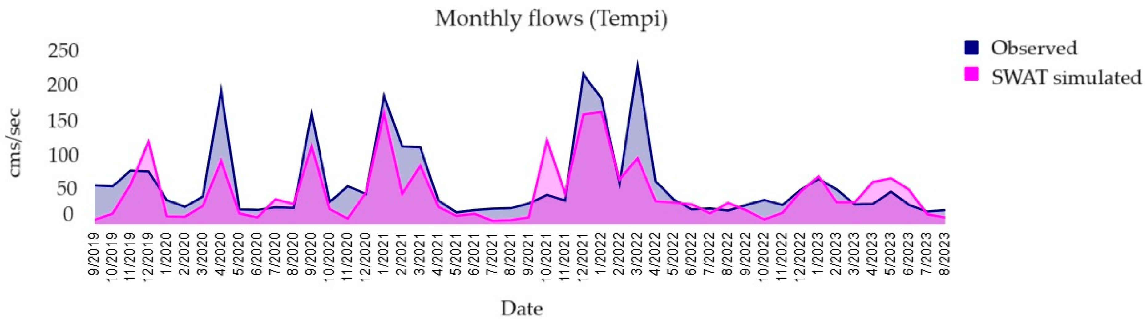
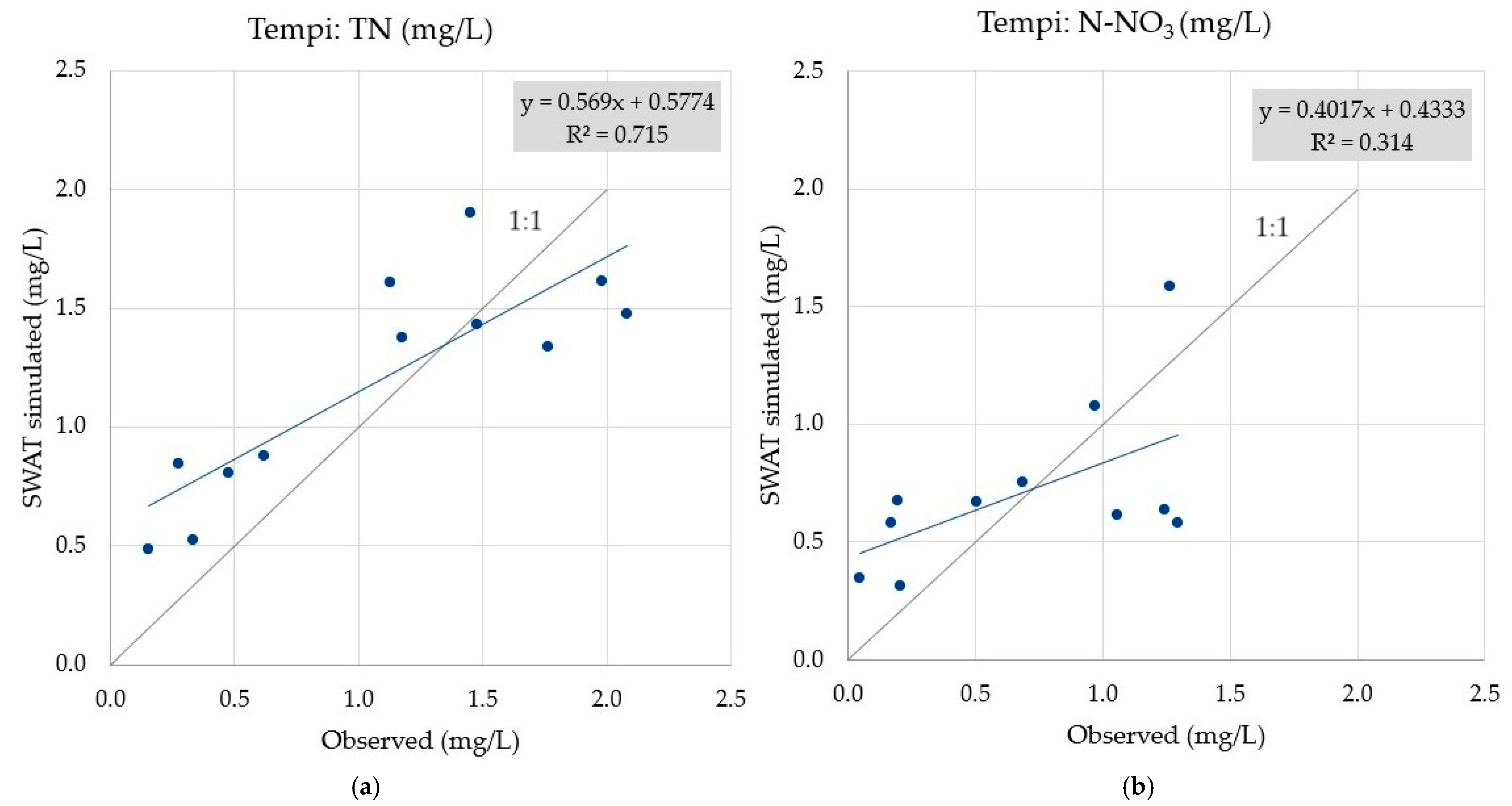
The PRB SWAT model developed in this study realistically simulated the hydrological and N cycle processes occurring at the river basin scale. Even though the N model predictions were only compared with river observations made at the basin’s outlet, the available data allowed for an adequate evaluation by the model at large time steps and for the entire basin. For the acceptance of the model predictions at nested sites of the basin, we had to rely on robust spatial parameterization of the model with respect to the land use, soil, and management.
This was the case for the crop yields and switchgrass biomass production in particular, as well as for the impact of switchgrass on water quality and quantity, for which it was essential to rely on other research studies with which to compare our model’s predictions. The reduction in surface runoff caused by the switchgrass implementation was the combined effect of (a) the more dense land coverage that characterizes most perennial crops compared to that of annual crops, resulting in reductions in surface runoff [56]; (b) the reduced amount of water that switchgrass received as irrigation, which also resulted in the production of less water capable of becoming runoff; and (c) the slightly increased ET, leaving a reduced amount of water to be lost via runoff [57].
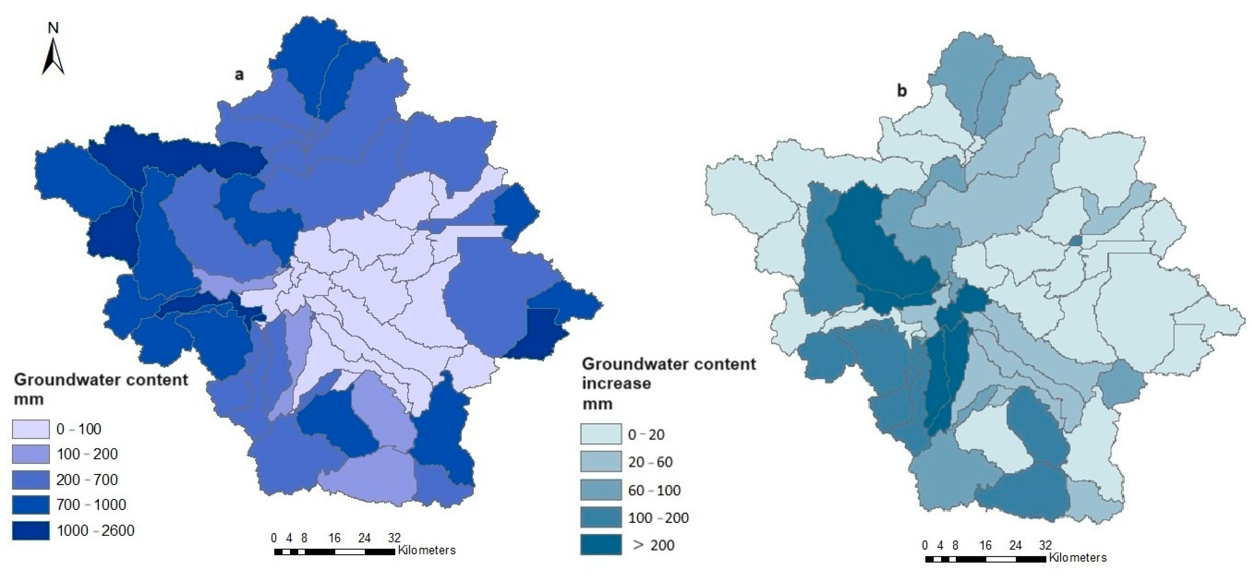
As has been stated, switchgrass received notably less irrigation water compared to that received by the existing irrigated crops in the PRB, which led to the assumption that its adoption could increase groundwater reserves. Indeed, apart from the reduced direct abstraction of water, in the majority of the HRUs, switchgrass was also able to reduce the surface runoff and increase the soil’s water content and percolation, the water that moves below the root zone over time [
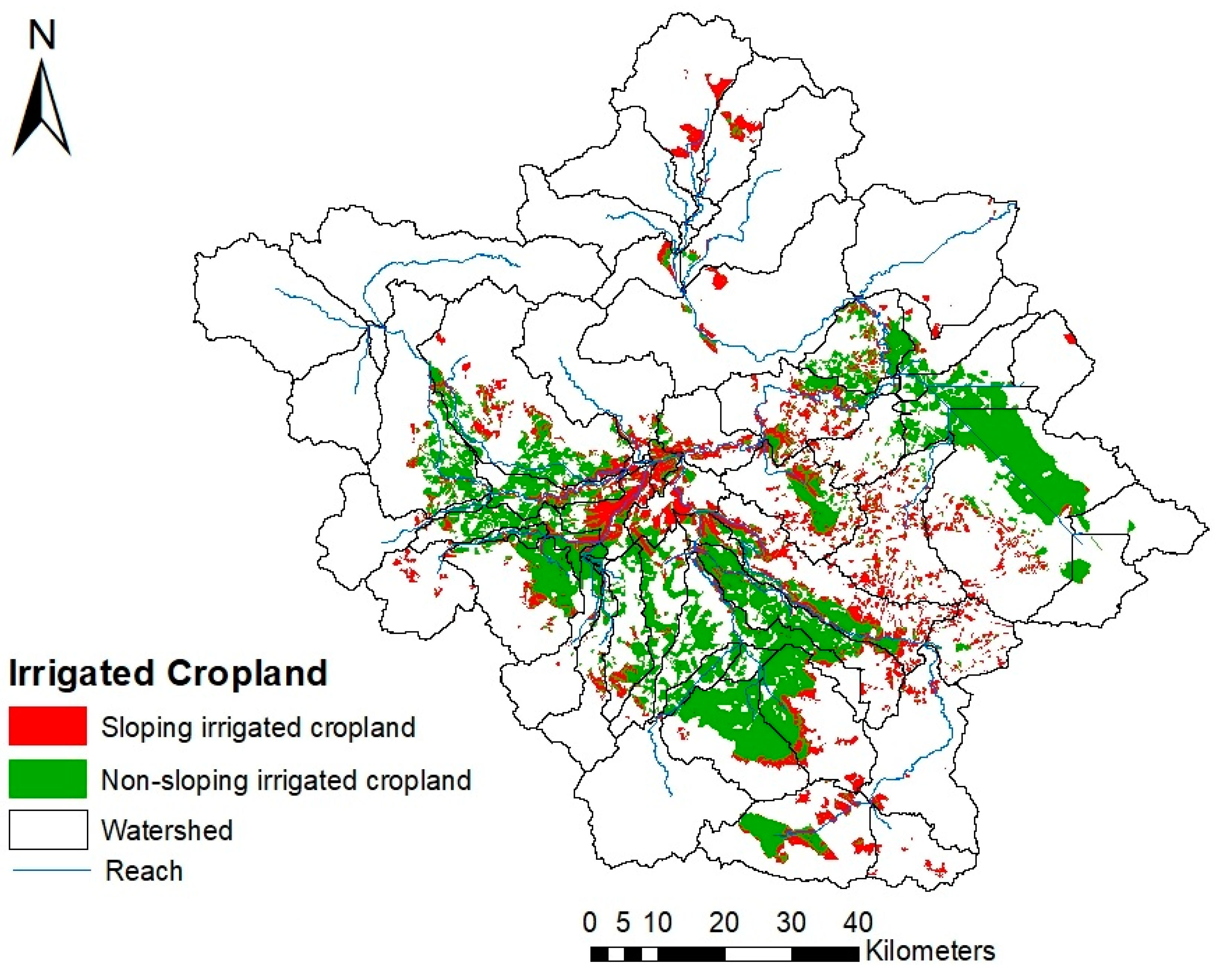
58]. While this was a fair observation at the entire basin level, there were certain HRUs where the opposite was observed due to less water being applied to the topsoil via irrigation. Overall, despite the fact that the areas that were available for the installation of switchgrass covered small percentages of the entire basin (19% of the basin represented the total irrigated cropland, 5.8% was the sloping irrigated cropland, and 13.2% was the non-sloping irrigated cropland), the individual effects in the subbasins were anything but trivial, as they proved to have the potential to improve the water availability considerably because of the reduced abstractions.
Regarding the total irrigation water used in the PRB, as expected, the effect of the fourth scenario (switchgrass in non-sloping irrigated cropland) was greater than the effect of the third scenario (sloping irrigated cropland), and this difference was attributed to the significantly greater area of non-sloping irrigated land that was available for the installation of switchgrass in the fourth scenario. This resulted in the replacement of more crops with greater irrigation water needs. Based on all of these results concerning the hydrology of the area in all of the developed scenarios, it can be concluded that the perennial crop could be effective in alleviating the high water abstraction from the shallow aquifers of the PRB and in this manner enhancing their water balance.
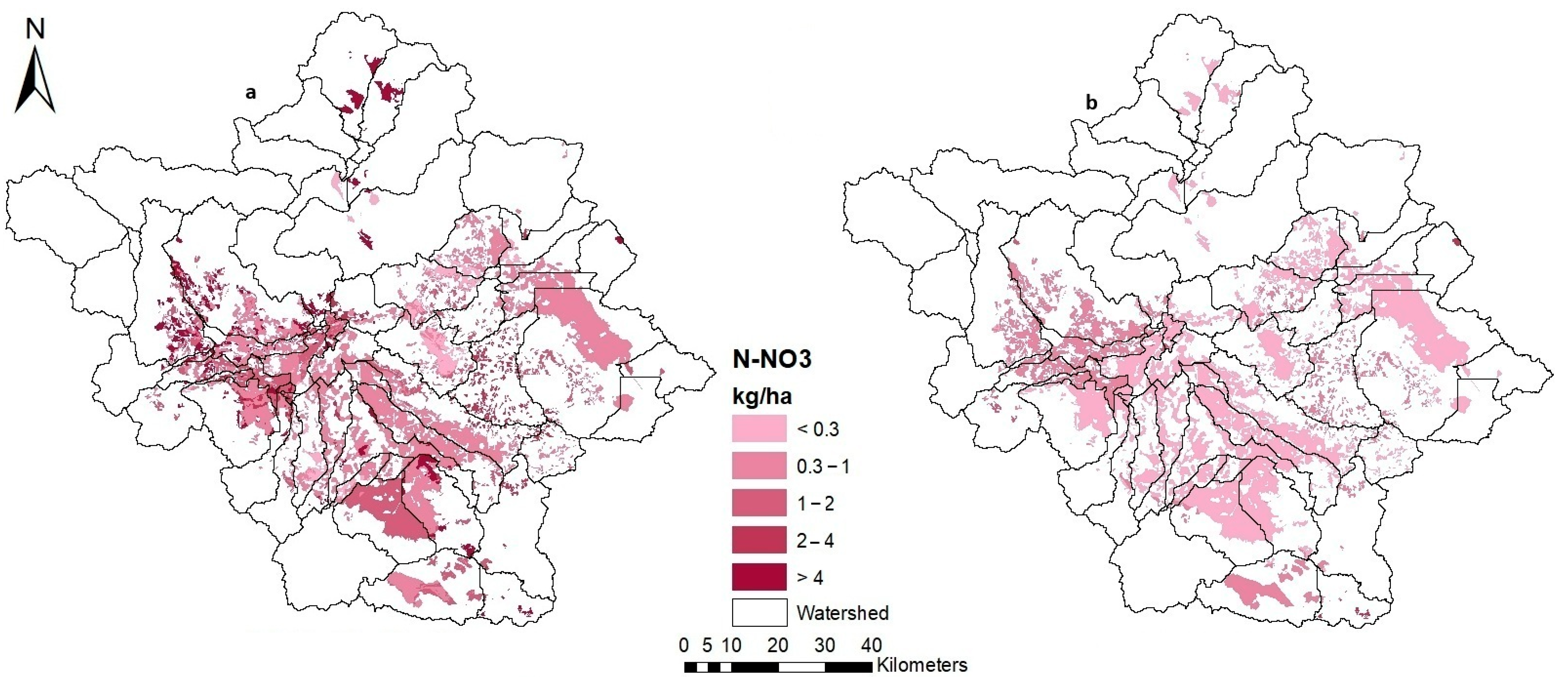
The agricultural use of N fertilizers has been a major contributor to the N export into the water from agricultural areas. Specifically, in PRB, which is highly vulnerable to N-NO3 pollution, N-NO3 reduction was considered to be of great importance. The trend in the N loss reduction was correlated with the N transported in dissolved form via runoff (mainly N-NO3). In general, the decrease in N-NO3 loading was mainly because switchgrass required a lower N fertilizer input in comparison to that for the baseline crops. The model simulations indicated that the adoption of the biofuel crop could reduce the N losses compared to those in the current cropping systems used in PRB, as observed in other studies as well [17,19,59,60]. The level of the reduction varied between scenarios, with the areal extent of the deployment of the bioenergy crop being the key factor for the greatest reduction being caused by the second scenario (with all irrigated crops replaced with switchgrass). However, the third and the fourth scenarios had the same overall effect at the basin level, resulting in average N-NO3 loss rates of 1.37 and 1.38 kg/ha, even though a lower rate was expected in the fourth scenario with switchgrass implemented in double the area compared to that in the third scenario. The almost identical N-NO3 reduction is obviously attributed to the greatest effect of the perennial crop in sloping areas where an increased reduction in runoff led to a more pronounced N-NO3 reduction as well. The rather low N-NO3 percentage reduction of 7% (1.37 and 1.38 from 1.48 kg/ha as shown in Table 10) was considerable for both scenarios since the conventional crop replacement represented a small percentage of land cover change in the entire basin (5.8% for the sloping irrigated cropland scenario and 13% for the non-sloping irrigated cropland scenario), and additionally, in both scenarios, there were extensive areas of non-irrigated wheat, not replaced by switchgrass, that still contributed greatly to N pollution (wheat HRUs contributed 47% of the total N-NO3 pollution from the cropland in the first baseline scenario). So, even though the effect was not as significant at the entire basin level as in the irrigated HRUs, if the perennial crop was planned to be installed in the entire sloping cropland (irrigated and non-irrigated), the N-NO3 could be reduced substantially, probably leading to impressive water quality improvements.
Nitrate pollution in PRB had anthropogenic activities as its main sources, mostly crop cultivation and secondly livestock farming. In groundwater, nitrate pollution is generally caused by the accumulation of nitrates, which in some cases can reach levels that are prohibitive to the use of water for water supply purposes. This means that the magnitude of N-NO3 leaching is directly or indirectly governed by N fertilization, N crop uptake, and the N lost from the soil that is transported into streams. Additionally, the increased concentration of leaching nitrates can be attributed to the high irrigation rates in these areas [61,62]. Thus, the reduced leached N-NO3 concentrations due to the switchgrass implementation were expected, as the perennial crop could reduce the N-NO3 leaching from the agricultural lands in our study area significantly due to its lower irrigation and N fertilization needs.
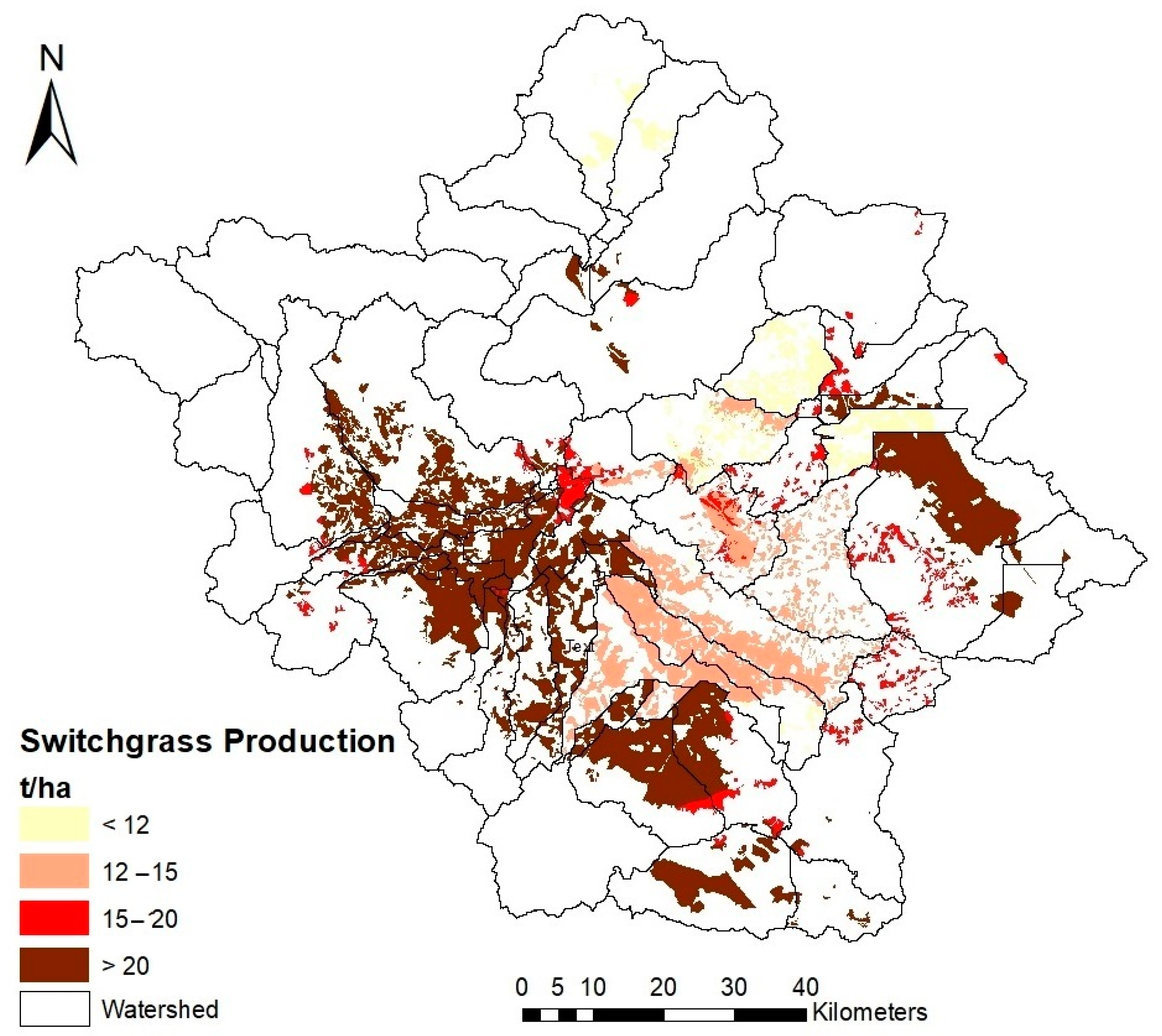
One limitation of SWAT in the simulation of crop growth is its inability to account for crop diseases in specific areas and years that may have led to relatively higher simulated yields in certain years than those reported. Hence, it is always preferred to discuss the simulated average annual yields, and this was the case for the switchgrass biomass production simulated under these scenarios. By calculating the biomass yields in sloping areas only, it could be concluded that some of the highest yields occurred there. Evidently, switchgrass had great potential to grow in these areas. The average biomass production calculated in the sloping land scenario was 18.2 t/ha, and the maximum production observed in a single HRU was 22 t/ha. The areas where inadequate production (of less than 12 t/ha) was observed (Figure 7) could be related to irrigation water deficits in these areas. In the center of the basin where the main part of the Thessaly plain (lowland areas) is located, there were constant biomass production yields of less than 15 t/ha (Figure 7). This can be also attributed to the insufficient groundwater content of the aquifers in this subregion due to the lower precipitation levels in this area, which has subsequently led to less percolation and aquifer recharge compared to those in other areas in the western parts of the basin. The deficit irrigation observed further proved that irrigation water was the main limiting parameter for switchgrass crop growth, as was stated by Giannoulis et al. [63] about this particular subregion of the PRB. It should be also noted that all of the irrigated areas served by reservoirs in this study had no problems with irrigation water shortages. A representative example of the positive role of reservoirs in meeting irrigation water needs in the PRB is the large area irrigated by the Karla reservoir in the most eastern part, where despite low precipitation and groundwater recharge, the switchgrass biomass production reached its maximum values of >20 t/ha/y (Figure 7).
Concerning the conventional irrigated crops in the PRB, their spatially averaged simulated yield rates per ha of cropland in the last two scenarios, when only part of the irrigated land was replaced with switchgrass, did not practically change from their average (per unit area) simulated yields at the baseline. However, an added benefit that was observed at the very local level under the partial replacement of irrigated conventional crops with switchgrass in the third and fourth scenarios was the increased availability of groundwater due to the reduced overall abstraction. The implementation of switchgrass solely in sloping/non-sloping irrigated areas offered the potential for the production yields of the adjacent conventional crops in non-sloping/sloping areas that were irrigated inadequately before to be improved due to the increased amounts of irrigation applied from groundwater.

5. Conclusions

The purpose of this study was to provide estimates of the effects that switchgrass cultivation could have on the water quantity and quality when implemented in large areas of a Greek agricultural basin using SWAT. The bioenergy crop proved to have great potential to grow in sloping areas and produce sufficient amounts of biomass, even though these areas were expected to have a relatively lower productivity due to their higher susceptibility to soil and nutrient losses. Specifically, the N-NO3 reductions at the basin level varied between 7 and 18% depending on the extent of deployment of the bioenergy crop, while there were individual HRUs with switchgrass installed where these reductions were greater than 80%. Implementing switchgrass on sloping land proved to be very effective in reducing the N-NO3 loads. Furthermore, the cultivation of the bioenergy crop could significantly alleviate the irrigation water abstraction by 10–40% depending on the replaced crops and the areal extent of the bioenergy crop’s installation. As a result, switchgrass increased the groundwater availability at several subbasins; specifically, for groundwater bodies in the most intensively irrigated central part of the basin, this increase was locally even higher than 50%.
Indeed, this study supports the progressive substitution of parts of the cropland containing conventional crops with bioenergy crops, promoting them as an effective restoration measure for water bodies, according to the WFD requirements, that could be also adopted in the next phases of regional WFD management plans. Ongoing research activities such as an economic analysis and the development of an efficient optimization tool could add value to the preliminary results presented in this paper, as they will allow additional criteria to be taken into consideration when selecting the locations for switchgrass implementation. It is believed that this current study on switchgrass simulation using SWAT, along with future directions, constitutes a useful approach to hydrological, water quality, and bioenergy crop simulations that could help decision-makers and water managers incorporate bioenergy crops into their combined efforts towards renewable energy production and water protection.

Author Contributions

Conceptualization: M.S., L.K. and Y.P. Methodology: M.S., L.K., K.D.G. and Y.P. Software: M.S., L.K., S.K. and H.G. Validation: M.S., L.K., S.K., H.G. and K.D.G. Formal analysis: M.S., L.K. and Y.P. Investigation: M.S., L.K., S.K., H.G. and E.D. Resources: M.S., L.K. and Y.P. Data curation: M.S., L.K., K.D.G., E.D. and Y.P. Writing—original draft preparation: M.S. and L.K. Writing—review and editing: M.S., L.K., S.K., H.G., K.D.G., E.D. and Y.P. Visualization: M.S., L.K., S.K., H.G. and Y.P. Supervision: Y.P. Project administration: Y.P. Funding acquisition: Y.P. All authors have read and agreed to the published version of the manuscript.

Funding

This research study was carried out within the framework of the National Recovery and Resilience Plan Greece 2.0, funded by the European Union—NextGenerationEU (Implementation body: HFRI). More specifically, this research was supported under the Basic Research Financing Action “Horizontal support of all sciences”, Sub-action 1 (Project Number: 16425; project title: BIOGRASS).

Data Availability Statement

The data used in this study are available from the authors of this paper upon request.

Acknowledgments

We would like to thank the reviewers for their constructive and insightful comments that helped us improve our article.

Conflicts of Interest

The authors declare no conflicts of interest.

References

  1. Claro, A.M.; Fonseca, A.; Fraga, H.; Santos, J.A. Future Agricultural Water Availability in Mediterranean Countries under Climate Change: A Systematic Review. Water 2024, 16, 2484. [Google Scholar] [CrossRef]
  2. Panagopoulos, Y.; Karpouzos, D.; Georgiou, P.; Papamichail, D. Ecosystem Services Evaluation from Sustainable Water Management in Agriculture: An Example from An Intensely Irrigated Area in Central Greece. In Proceedings of the 7th International Electronic Conference on Water Sciences, Online, 15–30 March 2023. [Google Scholar] [CrossRef]
  3. Malamataris, D.; Tsavdaridou, A.I.; Banti, D.; Malliaras, A.; Karalis, A.; Theocharis, N.; Michos, C.; Mazaris, A. Water-Ecosystems-Food nexus security achievement in the context of climate change: The case study of an agricultural Mediterranean Basin, Greece. Res. Ideas Outcomes 2023, 9, e116070. [Google Scholar] [CrossRef]
  4. De Girolamo, A.M.; Lo Porto, A. Source Apportionment of Nutrient Loads to a Mediterranean River and Potential Mitigation Measures. Water 2020, 12, 577. [Google Scholar] [CrossRef]
  5. Psomas, A.; Dagalaki, V.; Panagopoulos, Y.; Konsta, D.; Mimikou, M. Sustainable agricultural water management in Pinios river basin using remote sensing and hydrologic modeling. Procedia Eng. 2016, 162, 277–283. [Google Scholar] [CrossRef]
  6. Hellenic Ministry for the Environment, Energy and Climate Change—Special Secretariat for Water. Report on Directive 91/676/EEC—Nitrate Pollution Situation in the Greek Territory (Reference Period: 2020–2023). Available online: https://wfdver.ypeka.gr/wp-content/uploads/2017/04/files/GR08/GR08_P26b_Perilipsi_En.pdf (accessed on 10 October 2024).
  7. Skoulou, V.; Mariolis, N.; Zanakis, G.; Zabaniotou, A. Sustainable management of energy crops for integrated biofuels and green energy production in Greece. Renew. Sustain. Energy Rev. 2011, 15, 1928–1936. [Google Scholar] [CrossRef]
  8. Boukis, I.; Vassilakos, N.; Kontopoulos, G.; Karellas, S. Policy plan for the use of biomass and biofuels in Greece: Part I: Available biomass and methodology. Renew. Sustain. Energy Rev. 2009, 13, 971–985. [Google Scholar] [CrossRef]
  9. Mitkidis, G.; Magoutas, A.; Kitsios, F. Market and economic feasibility analysis for the implementation of 2nd generation biofuels in Greece. Energy Strat. Rev. 2018, 19, 85–98. [Google Scholar] [CrossRef]
  10. Giannoulis, K.; Bartzialis, D.; Skoufogianni, E.; Gravalos, I.; Xiradakis, P.; Danalatos, N.G. Panicum virgatum L. could be an alternative environmentally friendly feedstock for energy production. SSRG Int. J. Agric. Environ. Sci. 2017, 4, 14–23. [Google Scholar] [CrossRef]
  11. Chen, Y.; Marek, G.W.; Marek, T.H.; Moorhead, J.E.; Heflin, K.R.; Brauer, D.K.; Gowda, P.H.; Srinivasan, R. Assessment of alternative agricultural land use options for extending the availability of the Ogallala Aquifer in the Northern High Plains of Texas. Hydrology 2018, 5, 53. [Google Scholar] [CrossRef]
  12. Panagopoulos, Y.; Makropoulos, C.; Gkiokas, A.; Kossida, M.; Evangelou, L.; Lourmas, G.; Michas, S.; Tsadilas, C.; Papageorgiou, S.; Perleros, V.; et al. Assessing the cost-effectiveness of irrigation water management practices in water stressed agricultural catchments: The case of Pinios. Agric. Water Manag. 2014, 139, 31–42. [Google Scholar] [CrossRef]
  13. First Revision of the Regional River Basin Management Plan. Available online: https://wfdver.ypeka.gr/wp-content/uploads/2017/12/EL08_SDLAP_APPROVED.pdf (accessed on 20 November 2024). (In Greek).
  14. Kharel, G.; Zhong, Y.; Will, R.E.; Zhang, T.; Zou, C.B. Potential Hydrological Impacts of Planting Switchgrass on Marginal Rangelands in South Central Great Plains. Water 2022, 14, 3087. [Google Scholar] [CrossRef]
  15. Kumar, E.; Saraswat, D.; Singh, G. Comparative analysis of bioenergy crop impacts on water quality using static and dynamic land use change modeling approach. Water 2020, 12, 410. [Google Scholar] [CrossRef]
  16. Feng, Q.; Chaubey, I.; Cibin, R.; Engel, B.; Sudheer, K.P.; Volenec, J.; Omani, N. Perennial biomass production from marginal land in the Upper Mississippi River Basin. Land Degrad. Dev. 2018, 29, 1748–1755. [Google Scholar] [CrossRef]
  17. Panagopoulos, Y.; Gassman, P.W.; Kling, C.L.; Cibin, R.; Chaubey, I. Water quality assessment of large-scale bioenergy cropping scenarios for the upper Mississippi and Ohio-Tennessee river basins. JAWRA J. Am. Water Resour. Assoc. 2017, 53, 1355–1367. [Google Scholar] [CrossRef]
  18. Cibin, R.; Trybula, E.; Chaubey, I.; Brouder, S.M.; Volenec, J.J. Watershed-scale impacts of bioenergy crops on hydrology and water quality using improved SWAT model. GCB Bioenergy 2016, 8, 837–848. [Google Scholar] [CrossRef]
  19. Gassman, P.W.; Valcu-Lisman, A.M.; Kling, C.L.; Mickelson, S.K.; Panagopoulos, Y.; Cibin, R.; Chaubey, I.; Wolter, C.F.; Schilling, K.E. Assessment of bioenergy cropping scenarios for the Boone River watershed in north central Iowa, United States. JAWRA J. Am. Water Resour. Assoc. 2017, 53, 1336–1354. [Google Scholar] [CrossRef]
  20. Mentzafou, A.; Papadopoulos, A.; Dimitriou, E. Assessing the Impacts of Climatic and Water Management Scenarios in a Small Mountainous Greek River. Hydrology 2025, 12, 13. [Google Scholar] [CrossRef]
  21. Udias, A.; Pastori, M.; Malago, A.; Vigiak, O.; Nikolaidis, N.P.; Bouraoui, F. Identifying efficient agricultural irrigation strategies in Crete. Sci. Total. Environ. 2018, 633, 271–284. [Google Scholar] [CrossRef]
  22. Samarinas, N.; Tziolas, N.; Zalidis, G. Improved Estimations of Nitrate and Sediment Concentrations Based on SWAT Simulations and Annual Updated Land Cover Products from a Deep Learning Classification Algorithm. ISPRS Int. J. Geo-Inf. 2020, 9, 576. [Google Scholar] [CrossRef]
  23. Pisinaras, V.; Herrmann, F.; Panagopoulos, A.; Tziritis, E.; McNamara, I.; Wendland, F. Fully Distributed Water Balance Modelling in Large Agricultural Areas—The Pinios River Basin (Greece) Case Study. Sustainability 2023, 15, 4343. [Google Scholar] [CrossRef]
  24. Hellenic Statistical Authority, Data on Crop Areas. Available online: https://www.statistics.gr/en/statistics/-/publication/SPG06/- (accessed on 21 December 2024).
  25. Arampatzis, G.; Panagopoulos, A.; Pisinaras, V.; Tziritis, E.; Wendland, F. Identifying potential effects of climate change on the development of water resources in Pinios River Basin, Central Greece. Appl. Water Sci. 2018, 8, 51. [Google Scholar] [CrossRef]
  26. Vasiliades, L.; Loukas, A.; Liberis, N. A water balance derived drought index for Pinios River Basin, Greece. Water Resour. Manag. 2010, 25, 1087–1101. [Google Scholar] [CrossRef]
  27. Nitrates Directive—Vulnerable Zones Reporting 7—Web Map by Joint Research Centre of European Commission. Available online: https://water.jrc.ec.europa.eu/portal/apps/webappviewer/index.html?id=b33a220c1b284583851e93a245da02ef (accessed on 10 December 2024).
  28. Hellenic Ministry for the Environment, Energy and Climate Change-Special Secretariat for Water. Compilation of Management Plan for the River Basins of Thessaly Water District (GR08)-Management Plan; Athens, Greece, 2017. p. 252. Available online: https://wfdver.ypeka.gr/el/project/gr08-26b-approved-management-summaryen-gr/ (accessed on 15 November 2024).
  29. Second Revision of the Regional River Basin Management Plan. Available online: https://wfdver.ypeka.gr/wp-content/uploads/2024/07/EL08_2REV_sdlap.pdf (accessed on 25 November 2024). (In Greek).
  30. Williams, J.R.; Arnold, J.G.; Kiniry, J.R.; Gassman, P.W.; Green, C.H. History of model development at Temple, Texas. Hydrol. Sci. J. 2008, 53, 948–960. [Google Scholar] [CrossRef]
  31. Aloui, S.; Mazzoni, A.; Elomri, A.; Aouissi, J.; Boufekane, A.; Zghibi, A. A review of Soil and Water Assessment Tool (SWAT) studies of Mediterranean catchments: Applications, feasibility, and future directions. J. Environ. Manag. 2023, 326, 116799. [Google Scholar] [CrossRef]
  32. Neitsch, S.L.; Arnold, J.G.; Kiniry, J.R.; Williams, J.R. Soil and Water Assessment Tool (SWAT) Theoretical Documentation. Blackland Research Center, Texas. 2009. Agricultural Experiment Station, Temple, Texas (BRC Report 02–05). Available online: https://swat.tamu.edu/media/69296/swat-io-documentation-2012.pdf (accessed on 2 November 2024).
  33. Williams, J.R. Sediment-yield prediction with universal equation using runoff energy factor¹. In Present and Prospective Technology for Predicting Sediment Yield and Sources, Proceedings of the Sediment-Yield Workshop, USDA Sedimentation Laboratory, Oxford, MS, USA, 28–30 November 1972. Agricultural Research Service, US Department of Agriculture: 1975; Volume 40, p. 244. Oxford, MS, USA; Available online: https://upload.wikimedia.org/wikipedia/commons/e/e1/FEDLINK_-_United_States_Federal_Collection_%28IA_presentprospecti40sedi%29.pdf (accessed on 13 December 2024).
  34. Wischmeier, W.H.; Smith, D.D. Predicting rainfall-erosion losses from cropland east of the Rocky Mountains. In Agricultural Handbook; Agricultural Research Service: Washington, DC, USA, 1965; p. 282. [Google Scholar]
  35. Arabi, M.; Frankenberger, J.R.; Engel, B.A.; Arnold, J.G. Representation of agricultural conservation practices with SWAT. Hydrol. Process. Int. J. 2008, 22, 3042–3055. [Google Scholar] [CrossRef]
  36. Trybula, E.M.; Cibin, R.; Burks, J.L.; Chaubey, I.; Brouder, S.M.; Volenec, J.J. Perennial rhizomatous grasses as bioenergy feedstock in SWAT: Parameter development and model improvement. GCB Bioenergy 2015, 7, 1185–1202. [Google Scholar] [CrossRef]
  37. Jiang, R.; Wang, T.T.; Shao, J.; Guo, S.; Zhu, W.; Yu, Y.J.; Chen, S.; Hatano, R. Modeling the biomass of energy crops: Descriptions, strengths and prospective. J. Integr. Agric. 2017, 16, 1197–1210. [Google Scholar] [CrossRef]
  38. Corine Land Cover 2012—European Environment Agency. Available online: https://www.eea.europa.eu/data-and-maps/data/external/corine-land-cover-2012 (accessed on 15 November 2024).
  39. Hiederer, R. Mapping Soil Properties for Europe-Spatial Representation of Soil Database Attributes. EUR26082EN Scientific and Technical Research Series, 2013, Volume 47, pp. 1831–9424. Available online: https://citeseerx.ist.psu.edu/document?repid=rep1&type=pdf&doi=f0031d732307a43e9dca04e46b47dfc6d75a8be9 (accessed on 21 November 2024).
  40. Hiederer, R. Mapping Soil Typologies—Spatial Decision Support Applied to European Soil Database. Publications Office of the European Union, 2013, p. 127. Available online: https://esdac.jrc.ec.europa.eu/ESDB_Archive/eusoils_docs/other/EUR25932EN.pdf (accessed on 21 November 2024).
  41. Hellenic Statistical Authority, Data on Livestock. Available online: https://www.statistics.gr/en/statistics/-/publication/SPK13/- (accessed on 5 December 2024).
  42. General Secretariat of Waste Management Coordination, Wastewater Treatment Control and Planning Department, Web Map of the Urban Wastewater Treatment Plants. Available online: https://astikalimata.ypeka.gr/wtp (accessed on 20 November 2024).
  43. First Revision of River Basin Management Plans, Detailed Methodologies on Anthropogenic Pressures. Available online: https://wfdver.ypeka.gr/wp-content/uploads/2017/04/Methodologia_Piesewn_v3.pdf (accessed on 4 November 2024). (In Greek).
  44. Inland Water Department of the Hellenic Centre for Marine Research (HCMR), Data on the Automatic Monitoring Network of Hydrological Stations. Available online: https://hydro-stations.hcmr.gr/ (accessed on 5 November 2024).
  45. Oo, H.T.; Zin, W.W.; Kyi, C.T. Analysis of streamflow response to changing climate conditions using SWAT model. Civ. Eng. J. 2020, 6, 194–209. [Google Scholar] [CrossRef]
  46. Panagopoulos, Y.; Dimitriou, E. A Large-Scale Nature-Based Solution in Agriculture for Sustainable Water Management: The Lake Karla Case. Sustainability 2020, 12, 6761. [Google Scholar] [CrossRef]
  47. Desai, S.; Singh, D.K.; Islam, A.; Sarangi, A. Multi-site calibration of hydrological model and assessment of water balance in a semi-arid river basin of India. Quat. Int. 2021, 571, 136–149. [Google Scholar] [CrossRef]
  48. Moriasi, D.N.; Arnold, J.G.; Van Liew, M.W.; Bingner, R.L.; Harmel, R.D.; Veith, T.L. Model evaluation guidelines for systematic quantification of accuracy in watershed simulations. Trans. ASABE 2007, 50, 885–900. [Google Scholar] [CrossRef]
  49. Mapes, K.L.; Pricope, N.G. Evaluating SWAT model performance for runoff, percolation, and sediment loss estimation in low-gradient watersheds of the Atlantic coastal plain. Hydrology 2020, 7, 21. [Google Scholar] [CrossRef]
  50. Panagopoulos, Y.; Makropoulos, C.; Baltas, E.; Mimikou, M. SWAT parameterization for the identification of critical diffuse pollution source areas under data limitations. Ecol. Model. 2011, 222, 3500–3512. [Google Scholar] [CrossRef]
  51. WFD Program Conducted by Hellenic Centre for Marine Research HCMR. Monitoring and Recording of the Status (Quality, Quantity, Pressures, and Uses) of Surface Waters of Greece” (MIS 5001676), Under the Operational Program: “Transport Infrastructure, Environment and Sustainable Development” 2014–2020, Financed by the Hellenic Ministry of the Environment and the European Regional Development Fund. Available online: https://wfd.hcmr.gr/ (accessed on 16 November 2024).
  52. Skoulikidis, N.T.; Amaxidis, Y.; Bertahas, I.; Laschou, S.; Gritzalis, K. Analysis of factors driving stream water composition and synthesis of management tools—A case study on small/medium Greek catchments. Sci. Total. Environ. 2006, 362, 205–241. [Google Scholar] [CrossRef]
  53. Giannoulis, K.D.; Vlontzos, G.; Karyotis, T.; Bartzialis, D.; Danalatos, N.G. Assessing the efficiency of switchgrass different cultural practices for pellet production. Land Use Policy 2014, 41, 506–513. [Google Scholar] [CrossRef]
  54. Giannoulis, K.D.; Karyotis, T.; Sakellariou-Makrantonaki, M.; Bastiaans, L.; Struik, P.C.; Danalatos, N.G. Switchgrass biomass partitioning and growth characteristics under different management practices. NJAS Wagening. J. Life Sci. 2016, 78, 61–67. [Google Scholar] [CrossRef]
  55. Elbersen, H.W.; Christian, D.G.; El Bassem, N.; Alexopoulou, E.; Pignatelli, V.; Van Den Berg, D. Switchgrass (Panicum virgatum L.) as an Alternative Energy Crop in Europe. Initiation of a Productivity Network. Final Report Fair 5-CT97-3701 “Switchgrass”, 2001, pp. 1–91. Available online: www.switchgrass.nl (accessed on 9 December 2024).
  56. Goldstein, J.; Tarhule, A.; Brauer, D. Simulating the hydrologic response of a semiarid watershed to switchgrass cultivation. Hydrol. Res. 2014, 45, 99–114. [Google Scholar] [CrossRef]
  57. Schilling, K.E.; Jha, M.K.; Zhang, Y.K.; Gassman, P.W.; Wolter, C.F. Impact of land use and land cover change on the water balance of a large agricultural watershed: Historical effects and future directions. Water Resour. Res. 2008, 44. [Google Scholar] [CrossRef]
  58. Chen, Y.; Ale, S.; Rajan, N.; Morgan, C.L.S.; Park, J. Hydrological responses of land use change from cotton (Gossypium hirsutum L.) to cellulosic bioenergy crops in the Southern High Plains of Texas, USA. GCB Bioenergy 2016, 8, 981–999. [Google Scholar] [CrossRef]
  59. Chen, Y.; Ale, S.; Rajan, N.; Srinivasan, R. Modeling the effects of land use change from cotton (Gossypium hirsutum L.) to perennial bioenergy grasses on watershed hydrology and water quality under changing climate. Agric. Water Manag. 2017, 192, 198–208. [Google Scholar] [CrossRef]
  60. Femeena, P.V.; Sudheer, K.P.; Cibin, R.; Chaubey, I. Spatial optimization of cropping pattern for sustainable food and biofuel production with minimal downstream pollution. J. Environ. Manag. 2018, 212, 198–209. [Google Scholar] [CrossRef] [PubMed]
  61. Curk, M.; Glavan, M. Assessing and Mapping the Environmental Impacts of Best Management Practices in Nitrate-Vulnerable Areas. Water 2023, 15, 2364. [Google Scholar] [CrossRef]
  62. Yang, R.; Liu, W. Nitrate contamination of groundwater in an agroecosystem in Zhangye Oasis, Northwest China. Environ. Earth Sci. 2010, 61, 123–129. [Google Scholar] [CrossRef]
  63. Giannoulis, K.D.; Danalatos, N.G. Switchgrass (Panicum virgatum L.) nutrients use efficiency and uptake characteristics, and biomass yield for solid biofuel production under Mediterranean conditions. Biomass Bioenergy 2014, 68, 24–31. [Google Scholar] [CrossRef]
Figure 1. The location of Pinios river basin in Thessaly, central Greece, and a Digital Elevation Model of the basin with monitoring points and reservoirs.
Hydrology 12 00066 g001
Figure 2. Simulated vs. observed river flows (2019–2023) at Tempi station.
Hydrology 12 00066 g002
Figure 3. Total nitrogen (a) and N-NO3 (b) comparisons at the basin outlet Tempi.
Hydrology 12 00066 g003
Figure 4. Sloping (>1.5%) and non-sloping irrigated cropland map of Pinios river basin.
Hydrology 12 00066 g004
Figure 5. Groundwater content in the Pinios river basin at the end of the simulation period (end of 2023), expressed in mm of water for the baseline (a) and as the increase from the baseline (in mm) in the second scenario (b).
Hydrology 12 00066 g005
Figure 6. Mean annual (2018–2023) N-NO3 load of the irrigated cropland within Pinios river basin under (a) the baseline scenario and (b) the switchgrass implementation in all irrigated cropland scenarios.
Hydrology 12 00066 g006
Figure 7. Mean annual (2018–2023) switchgrass biomass production in t/ha in the second scenario (switchgrass implementation in the entire cropland).
Hydrology 12 00066 g007
Table 1. Distribution of cultivated crops in Pinios river basin.
Land UseArea (ha)Basin Percentage (%)
Alfalfa15,2871.4
Corn22,9082.0
Cotton164,49715.5
Fallow areas84,1597.9
Wheat165,63615.6
Table 2. Soil parameters in SWAT Pinios river basin model extracted from the European Soil Database [39,40].
SWAT Soil Layer ParametersSWAT Parameter DefinitionParameters of Datasets Based on ESDBDataset
SOL_BD1 (g/cm3)Moist bulk density in the first soil layer STU_EU_T_BDESDB-derived data
SOL_AWC1 (mm/mm)Available water capacity of the first soil layer(=FC-WP)3D soil hydraulic DB
SOL_CBN1 (% wt.)Organic carbon content in the first soil layerSTU_EU_T_OCESDB-derived data
SOL_K1 (mm/h)Saturated hydraulic conductivity in the first soil layerKS3D soil hydraulic DB
CLAY1 (% wt.)Clay content in the first soil layerSTU_EU_T_CLAYESDB-derived data
SILT1 (% wt.)Silt content in the first soil layerSTU_EU_T_SILT
SAND1 (% wt.)Sand content in the first soil layerSTU_EU_T_SAND
ROCK1 (% wt.)Roch Fragment content in the first soil layerSTU_EU_T_GRAVEL
USLE_K1USLE equation soil erodibility (K) factor in the first soil layerK_factor_soiltexture_WischmeierGlobal soil erodibility
Table 3. Summarized information on the data used for the schematization, parameterization, and performance evaluation of the Pinios river basin SWAT model.
DatasetDescription of the Data
Topography25 × 25 m Digital Elevation Model (DEM) data used to delineate the area and the river network
Land use1:100,000 land cover layer derived from Corine 2012; crop patterns evaluated from the Hellenic Statistical Authority (ELSTAT) for the years 2012–2021
Soil1 × 1 km soil map produced using information provided by the European Soil Database (ESDB)
Daily climateDaily precipitation, maximum and minimum temperature, relative humidity, and wind speed data from 31 stations during the years 2016–2023
Crop parametersPlant parameters needed for the SWAT plant database were provided by assistant professor at the School of Agriculture of the University of Thessaly Kyriakos Giannoulis (co-author of this article)
Point sourcesPoint source data were collected from the official website of the Ministry of Environment and Energy for the operation of the WWTPs, as well as from the Approved River Basin Management Plan of the Thessaly Water District (EL08)
Major dams/reservoirsKey reservoirs for main channels of the Pinios river and its tributaries (Smokovo, Girtoni, and Karla) and Plastiras reservoir located outside the basin
River flowDaily measured river flow data (in m3/s) accessible from the automatic monitoring network of hydrological stations of the Inland Water Department of the Hellenic Centre for Marine Research (HCMR) for the years 2016–2023
River water qualityObserved seasonal data related to N species concentrations in rivers acquired by the national monitoring program for the implementation of the WFD in Greece conducted by HCMR for the years 2018–2022
Crop yieldsReported values provided by the Hellenic Statistical Authority for the years 2011–2021
Table 4. Calibrated parameters used consistently in the Pinios river basin model.
IDParameterOptimum Value
1GWQMIN (mm)1000
2GW_REVAP0.02
3REVAPMN (mm)750
4GW_DELAY (days)31
5CN2Ranging from 65.05 to 82.65 depending on the land use and soil type
6SOL_AWC (mm)0.11–0.17 water/mm soil for each layer depending on the soil type
7SOL_K (mm/h)8.2–21.69 for each layer depending on the soil type
8SHALLST (mm)0
GWQMIN: threshold for the depth of water in a shallow aquifer required for return flow to occur (mm); GW_REVAP: groundwater “revap” coefficient; REVAPMN: threshold for the depth of water in a shallow aquifer for “revap” or percolation into a deep aquifer to occur (mm); GW_DELAY: groundwater delay (days); CN2: initial SCS runoff curve number for moisture condition I; SOL_AWC: available water capacity of the soil layer (mm); SOL_K: saturated hydraulic conductivity (mm/h); SHALLST: initial depth of the water in a shallow aquifer (mm).
Table 5. The main optimum nitrogen parameters of the SWAT Pinios River basin model.
Variable NameDescriptionNormal RangeFinal Value
CDNDenitrification exponential rate coefficient0.0–3.00.1
SDNCODenitrification threshold water content0.1–1.10.997
NPERCON-NO3 percolation coefficient0.0–1.00.2
RCNConcentration of nitrogen in rainfall (mg N/L)-1
RCN_SUBAtmospheric deposition of nitrate (mg/L)-1
Table 6. Adjusted plant parameters for the four conventional crops in the Pinios river basin.
Variable NameDefinitionCottonWheatCornAlfalfa
HVSTIHarvest index for optimal growing conditions [(kg/ha)/(kg/ha)]0.50.40.60.8
WSYFLower limit of harvest index [(kg/ha)/(kg/ha)]0.50.20.50.6
BLAIMaximum potential leaf area index (LAI)5584
CHTMXMaximum canopy height (m)10.930.9
RDMXMaximum root depth1.511.53
T_OPTOptimum temperature28202625
T_BASEMinimum (base) temperature for plant growth (°C)14092
ALAI_MINMinimum leaf area index for plants during the dormant period (m2/m2)0000.5
C_USLEMinimum value of the USLE C-factor for the water erosion applicable to the land cover/plant0.20.030.20.03
HEAT UNITSTotal heat units for the cover/plant to reach maturity1700134227001264
Table 7. Switchgrass scenarios applied across the cropland of the Pinios river basin.
Scenario No.Description
1Baseline scenario
2Switchgrass in the entire irrigated cropland
3Switchgrass in irrigated sloping cropland
4Switchgrass in irrigated non-sloping cropland
Table 8. Sloping and non-sloping irrigated cropland distribution in Pinios river basin.
CategoryArea (ha)% Basin% Cropland% Irrigated Cropland
Basin1,062,270---
Cropland368,32834.7--
Irrigated cropland202,69219.055.0-
Irrigated sloping land61,1565.816.630.0
Irrigated non-sloping land141,53713.238.470.0
Table 9. Plant parameters adjusted for Alamo switchgrass.
Variable NameDefinitionSwitchgrass
HVSTIHarvest index for optimal growing conditions [(kg/ha)/(kg/ha)]0.95
BLAIMaximum potential leaf area index (LAI)9
CHTMXMaximum canopy height (m)2.5
RDMXMaximum root depth3
T_OPTOptimum temperature27
T_BASEMinimum (base) temperature for plant growth (°C)10
WSYFLower limit of harvest index [(kg/ha)/(kg/ha)]0.95
HEATUNITSTotal heat units for cover/plant to reach maturity2500
Table 10. SWAT estimates of water, N, and biomass production in Pinios river basin during 2018–2023 under the implementation of the four scenarios.
ParametersResults
Scenario 1Scenario 2Scenario 3Scenario 4
Average annual surface runoff (mm)157133150140
Average annual ET (mm)461470465466
Groundwater content at the end of the simulation period (106 m3)5610618058175914
Total annual irrigation water used (106 m3)680413616493
N-NO3 loss (kg/ha)1.481.211.371.38
N-leached (mg/L)21.211.916.415.9
Average annual switchgrass biomass production (t/ha)-18.618.218.4
Scenario 1: baseline scenario; Scenario 2: switchgrass implementation in the entire irrigated cropland; Scenario 3: switchgrass implementation in irrigated sloping cropland; and Scenario 4: switchgrass implementation in irrigated non-sloping cropland.
Disclaimer/Publisher’s Note: The statements, opinions and data contained in all publications are solely those of the individual author(s) and contributor(s) and not of MDPI and/or the editor(s). MDPI and/or the editor(s) disclaim responsibility for any injury to people or property resulting from any ideas, methods, instructions or products referred to in the content.

