Seasonal and Spatial Dynamics of Surface Water Resources in the Tropical Semi-Arid Area of the Letaba Catchment: Insights from Google Earth Engine, Landscape Metrics, and Sentinel-2 Imagery

Abstract

Understanding the spatial and seasonal dynamics of surface water bodies is imperative for addressing water security challenges in water-scarce regions. This study aimed to evaluate the efficacy of multi-date Sentinel-2-derived spectral indices, specifically the normalized difference water index (NDWI), modified normalized difference water index (MNDWI), and Sentinel 2 Water Index (SWI), in conjunction with landscape metrics for mapping spatial and seasonal fluctuations in surface water bodies. Google Earth Engine (GEE) was employed for this assessment. The research achieved impressive overall accuracies, ranging from 96 to 100% for both dry and wet seasons, highlighting the robustness of the methodology. The study revealed significant differences in water bodies in terms of size and coverage between the dry and wet seasons. Surprisingly, the dry season exhibited a higher prevalence of water bodies when compared to the wet season, indicating unexpected patterns of water availability in the region and the substantial heterogeneity of water bodies. Meanwhile, the wet season was characterized by extensive coverage. These findings challenge conventional assumptions about water resource availability during different seasons. Based on the findings, the study recommends that water resource management strategies in semi-arid regions consider the observed seasonal variability in water bodies. Policymakers and stakeholders should adopt adaptive management approaches to address the unique challenges posed by differing water body dynamics in dry and wet seasons. Future research endeavors should explore the underlying factors driving these seasonal fluctuations and assess the potential long-term impacts on water availability. This can help to develop more resilient and sustainable water security strategies to cope with changing climate conditions in semi-arid tropical environments.

1. Introduction

Surface water is the most accessible and irreplaceable natural resource, sustaining most organisms on the planet [1,2]. It plays a crucial role in livelihoods, socio-economic development, ecosystem services, and the circulation and exchange of Earth’s energy [2,3]. However, human activities have profoundly altered natural water resources through mechanisms such as urbanization and deforestation, leading to significant ecosystem and landscape changes. These disruptions affect natural water cycles, reducing the Earth’s capacity to regulate vital ecological processes [4].

Tropical semi-arid regions are particularly vulnerable due to their unpredictable weather, prolonged dry seasons, and inconsistent rainfall [5]. Surface water availability in these regions is subject to a complex interplay of climatic, geological, ecological, and anthropogenic factors [6,7]. With rising global temperatures, these areas are experiencing altered precipitation patterns, intensified droughts, and increased evapotranspiration, further exacerbating water scarcity [8,9]. Additionally, rapid population growth places immense pressure on already limited water resources, necessitating the exploration of effective water management strategies to prevent environmental degradation [10].

Accurate and up-to-date information on surface water distribution is essential for monitoring climate change impacts, predicting floods, assessing the factors that affect water variability, and quantifying water resource decline [2,11]. Due to the arid nature and irregular rainfall patterns of tropical semi-arid regions, the availability of surface water fluctuates significantly. Understanding the spatial and seasonal dynamics of water bodies is crucial for enhancing water security, particularly during dry periods when water scarcity is most severe. This knowledge contributes to effective water management strategies, enabling decision-makers to allocate resources efficiently and sustainably.

Remote sensing provides an efficient means of collecting data over large areas, allowing for the comprehensive assessment of water resources and their spatial patterns. Several studies have demonstrated its effectiveness in long-term surface water monitoring. [12] utilized Landsat 5 and 7 to map open water bodies in Oklahoma (1984–2015) using the Modified Normalized Difference Water Index (MNDWI) and Normalized Difference Water Index (NDWI). Similarly, [13] extracted water bodies in Lake Burdur, Turkey (1987–2011), using Support Vector Machines (SVM), NDWI, MNDWI, and the Automated Water Extraction Index (AWEI). [14] monitored the extent of surface water in the USA, Egypt, Ukraine, Brazil, and Canada using MODIS data and SVM. These studies highlighted high inter- and intra-annual variability in surface water resources, with temporary water bodies often going undetected due to their short-lived and erratic nature. Seasonal surface water can exhibit strong variation between wet and dry seasons, sometimes shifting geographically [5]. The majority of these studies relied on Landsat satellites for long-term monitoring of water bodies [15,16].

The availability of free satellite imagery from platforms such as Sentinel satellites has significantly improved water body monitoring [17]. However, few studies have leveraged these datasets for mapping and monitoring surface water [18,19]. These datasets provide consistent seasonal and long-term coverage, enabling a detailed analysis of water body changes over time. Water indices such as the NDWI and MNDWI have been widely used for water body delineation due to their spectral band effectiveness. However, slight variations in the spectral range of wavebands across different sensors can lead to discrepancies in water extraction results [18].

Sentinel-2, developed by the European Space Agency (ESA), is a state-of-the-art satellite system designed for Earth observation, with a particular focus on land and water resource monitoring. Its high spatial, spectral, and temporal resolution makes it ideal for mapping water bodies [18,19]. The multispectral advantages of Sentinel-2 include its 10 m resolution in visible and near-infrared bands and its red-edge bands, which enhance vegetation–water differentiation, minimizing classification errors in complex landscapes. This fine spatial detail enables the precise delineation of small water bodies and narrow rivers [18,19]. However, traditional desktop processing for remote sensing tasks such as mosaicking, image retrieval, and cloud filtering is time-intensive and poses significant challenges [20]. To overcome these challenges, cloud computing platforms like Google Earth Engine (GEE) provide powerful processing capabilities for monitoring and mapping surface water bodies. GEE integrates more than 200 remote sensing datasets and supports Python and JavaScript, enabling users to process and analyze data efficiently [21]. Studies have demonstrated GEE’s effectiveness in water monitoring; these include those by [22] for inland water bodies, [23] in India, and [24] in New Zealand, where Landsat and GEE were used for automated water body detection.

Landscape metrics are quantitative tools used to measure spatial patterns and structures within a landscape, such as the size, shape, and distribution of land cover patches [25]. These metrics are essential for monitoring water bodies, as they provide insights into water dynamics, water quality, and ecosystem health [26]. However, while widely applied in ecological studies, landscape metrics have been underutilized in surface water monitoring, despite their potential to assess seasonal fluctuations and landscape influences on hydrological processes. Analyzing landscape metrics at different times of the year is crucial for understanding how the surrounding land cover impacts water body dynamics during high and low water periods.

This study aims to address the critical need for the comprehensive monitoring of surface water resources in tropical semi-arid regions, particularly in Southern Africa, which faces increasing climate variability and anthropogenic pressures. Despite advancements in remote sensing, a significant research gap remains in understanding the seasonal and spatial dynamics of surface water in tropical semi-arid catchments like the Letaba. By leveraging the cloud-based capabilities of GEE to process and analyze Sentinel-2 imagery, this study enables the efficient detection and monitoring of surface water changes over time. Integrating landscape metrics further enhances the analysis by providing a detailed understanding of water body fragmentation and spatial configuration, offering valuable insights into how landscape patterns influence hydrological processes.

The Letaba catchment has experienced significant agricultural expansion in recent years, yet data on water availability, variability, pollution, and scarcity remain limited. To address this, the study aims to (i) seasonally detect and map the spatial distribution of surface water bodies in the Letaba catchment using Sentinel-2-derived spectral indices via the GEE platform, and (ii) quantify the seasonal spatial configuration of surface water bodies using landscape metrics. These objectives will contribute to a more comprehensive understanding of water resources in the region and support sustainable water management practices.

2. Materials and Methods

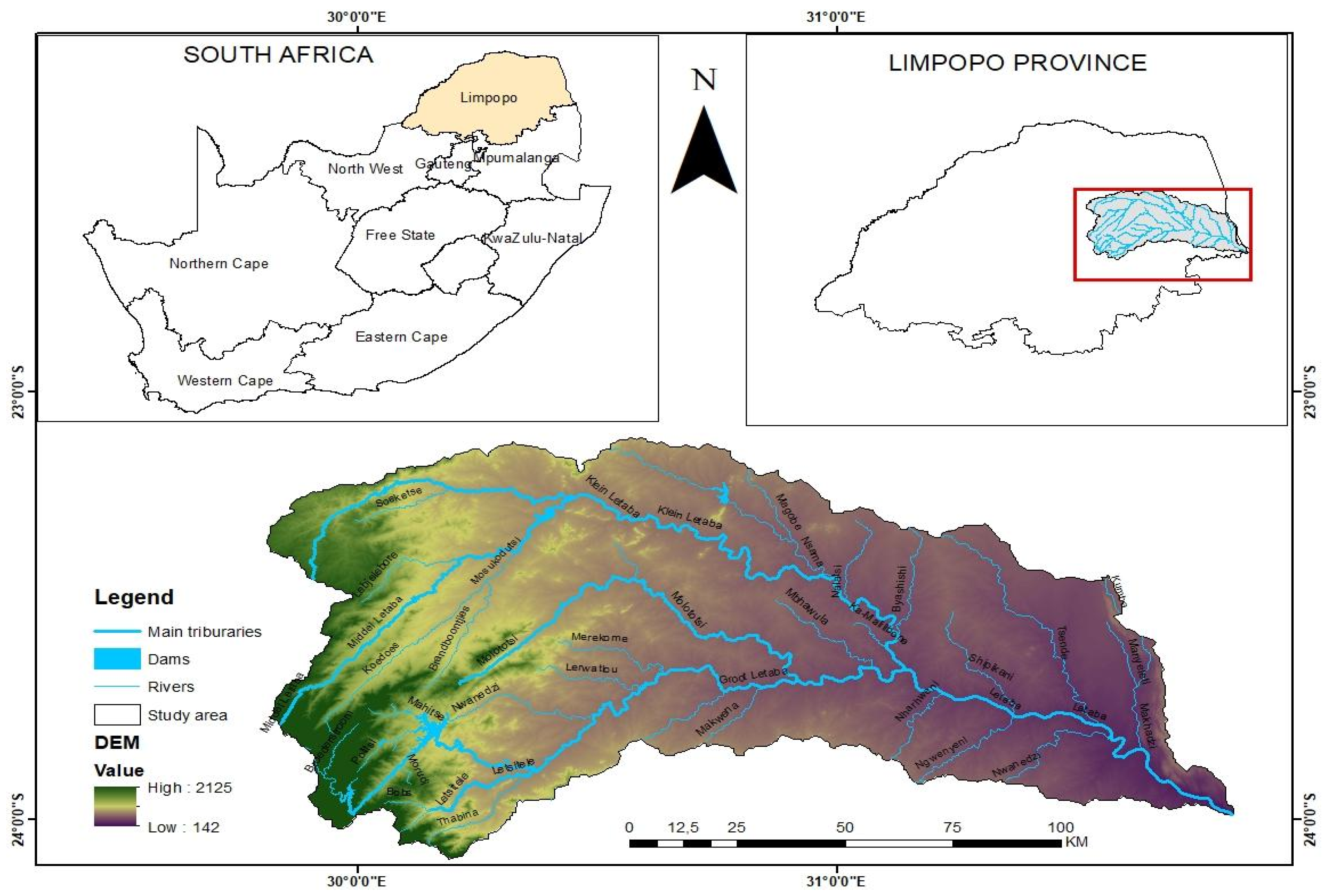
2.1. Study Area

The study took place within the Letaba watershed, positioned between the longitudes 30°0′ and 31°40′ East and latitudes 23°30′ and 24°0′ South, located in the Limpopo province of South Africa (as depicted in Figure 1). Covering an area of 1,451,864 hectares, the Letaba watershed experiences an average annual evapotranspiration ranging from 1100 mm to 1300 mm. The region receives between 300 mm and 400 mm of rainfall, with an annual runoff of 574 million cubic meters. The mean annual temperature ranges from a minimum of 18 °C to a maximum of 28 °C, differing between the mountainous and lowland areas. The main tributaries of the Groot Letaba River that drain into the catchment include the Klein Letaba, Middle Letaba, Molototsi, and Litsetele rivers [27]. The Letaba catchment has more than 20 constructed dams and weirs, leading to a high degree of regulation within the watershed. The available water resources within this area are overexploited to fulfill both domestic needs and commercial demands, such as afforestation, industrial use, and irrigation.

2.2. Data Acquisition and Analysis

This study, conducted from 2017 to 2022, utilized Sentinel-2 surface reflectance (SR) imagery, labeled as COPERNICUS/S2_SR within the GEE platform, to analyze surface water dynamics in the Letaba catchment. This dataset is available in the GEE cloud database and can be accessed at https://earthengine.google.com/ (accessed on 16 March 2025). The imagery consists of fourteen spectral bands with resolutions of 10 m, 20 m and 60 m, as shown in

Table 1. Detailed information of Sentinel 2 spectral bands.

Band Name	Band Number in GEE	Band Resolution
Coastal Aerosol	SR_B1	60
Green	SR_B2	10
Red	SR_B3	10
Blue	SR_B4	10
Vegetation Red Edge	SR_B5	20
Vegetation Red Edge	SR_B6	20
Vegetation Red Edge	SR_B7	20
Near-Infrared (NIR)	SR_B8	10
Narrow NIR	SR_B8A	20
Water Vapor	SR_B9	60
Shortwave Infrared 1 (SWIR-1)	SR_B11	20
Shortwave Infrared 2 (SWIR-2)	SR_B12	20
Shortwave Infrared 3 (SWIR-3)	SR_B13	20
Cloud Mask	QA60	60

. To define the region of interest (ROI), a vector dataset containing hydrographic basin geometries and names was imported into GEE. The ROI was specified using the geometry function. Cloud masking was performed using the maskClouds function, which removed atmospheric distortions such as clouds and shadows by applying the QA60 bands. The Sentinel-2 SR dataset was then loaded and filtered by date using the filterDate function, categorizing the data into dry and wet seasons. The wet season ranged from mid-September to March, while the dry season extended from April to mid-September. Additionally, the wet season was defined as mid-September of the previous year to March of the current year. For example, the 2017 wet season covered mid-September 2016 to March 2017, and so forth.

Filtered images were further refined to match the study area’s boundaries using the filterBounds function. The filtered images were then merged with the masked cloud data and processed to generate a median composite image, which averaged the date range of the selected images. Following this, the Normalized Difference Water Index (NDWI), Modified Normalized Difference Water Index (MNDWI), and Sentinel 2 Water Index (SWI) were computed using their respective formulas (Table 1), with the results stored in variables named the NDWI, MNDWI, and SWI. These indices were used to distinguish water bodies from non-water bodies.

For visualization, color palettes designated as “rgbVis” and “ndwiVis” were applied. Finally, the NDWI, MNDWI, and SWI layers were added to the map using the Map.addLayer function, utilizing the “ndwiVis” palette to effectively highlight surface water features. Additionally, the number of images used for mapping water bodies during the wet and dry seasons was counted.

2.3. Spectral Derived Indices

2.3.1. Extraction of Surface Water Bodies

Various water indices were tested in the Letaba catchment for the years 2017 to 2022 to distinguish water bodies from non-water bodies. The study included the commonly used water indices such as the Normalized Difference Water Index (NDWI), Modified Normalized Difference Water Index (MNDW), Sentinel 2 Water Index (SWI), Automated Water Extraction Index (AWEI) [6], Normalized Difference Vegetation Index (NDVI) [28], Normalized Difference Water Index (NDWI2) [29] and Modified Normalized Difference (MNDWI) using shortwave infrared (band 10). However, these indices were not effective in accurately extracting water bodies and resulted in significant misclassification in this area. Despite this, the NDWI, MNDWI, and SWI proved to be superior in capturing the spatial and seasonal dynamics of surface water bodies in the Letaba catchment. Therefore, we chose to use these indices for the final analysis, as they provided more accurate and reliable results.

The methods used to determine the water indices for water extraction were chosen based on their ability to use several reflectivity variations in the spectrum that differentiate water from non-water classes [30,31]. Moreover, they have been successfully used to extract water bodies due to their accuracy and can capture significant information on inter and intra-seasonal variations in surface water bodies [32,33]. However, in this case, water indices such as the normalized difference water index (NDWI), Sentinel 2 water index (SWI) and the modified normalized water index (MNDWI) were assessed as the most appropriate algorithms for outlining water bodies. These indices were compared against each other for delineating surface water bodies within the Letaba catchment.

Table 2. The spectral water indices used to extract surface water bodies in the Letaba catchment from sentinel 2.

Water Indices	Formulae	Threshold	Reference
Normalized difference water index (NDWI)	NDWI = (Green − NIR)/(Green + NIR)	NDWI > 0	[34]
Modified normalized difference water index (MNDWI)	MNDWI = (Green − SWIR2)/(Green + SWIR2)	MNDWI > 0	[35]
Sentinel 2 Water Index (SWI)	SWI = (Red edge − SWIR2)/(Red edge + SWIR2)	SWI > 0	[18]

presents the spectral indices applied to surface water bodies using imagery from the Sentinel 2 Multispectral Instrument (MSI) within the Letaba catchment.

2.3.2. Validation

A total of 300 referenced random points of water bodies and non-water bodies were generated and digitized using high-spatial-resolution imagery in Google Earth (GE). The digitized points were then imported into the GEE cloud computing platform to confirm whether they fell within or outside the produced water indices map generated in Google Earth Engine (GEE). The collected points were obtained during the same season as the Sentinel-2 image acquisition. Then, a confusion matrix was created to quantify the producer, user, and overall accuracy by identifying four variables of pixels:

• True positive (TP): number of accurate extracted water pixel points.
• False negative (FN): number of undetected water pixel points.
• False positive (FP): number of erroneously extracted water pixel points.
• True Negative (TN): number of non-water pixel points.
• Overall accuracy (%) = (TP + TN) × 100/Total number of pixel (T)

The producer, user, and overall accuracy show correct predictions and have a range of 0 to 100%, with a value close to 100 showing perfect accuracy [36] (Albarqouni et al., 2022).

2.4. Spatial Configuration

To assess the spatial arrangement of water bodies in relation to landscape characteristics, it is crucial to define and quantify the complexity of the landscape [7] (Tulbure and Broich, 2013). Four landscape metrics were selected to capture the key attributes of various water body levels. These metrics were chosen to illustrate the changes and enable a comparative analysis, facilitating an evaluation of the water body complexities within the Letaba catchment. The metrics used are as follows:

(i)

Number of Water Bodies (NW): This metric represents the total number of distinct water bodies within a defined area. Monitoring NW helps to understand the proliferation or reduction in aquatic habitats, influenced by factors such as climate change, land use changes, or conservation efforts. This metric was calculated by converting the raster (water image) into vector data using the reduceToVectors function in Google Earth Engine (GEE), applying the parameter ee.reducer.countEvery to count the number of water bodies within the study area.

(ii)

Mean Area of Water Bodies (MAW): This metric provides the average size of water bodies, offering insights into habitat availability and the potential to support biodiversity. Changes in MAW may indicate ecological shifts, such as the drying up of smaller ponds or the expansion of larger lakes. To calculate MAW, the area of each water body was determined using the GEE function area. The area in hectares was then calculated by dividing by 10,000 using the divide function. The average water body area was computed using the following formula:

MAW = ΣXi/NW

where Xi corresponds to the area of each water body within a given landscape, and NW represents the total count of water bodies in that landscape.

(iii)

Total Area of Water Bodies (TAW): This metric quantifies the total area covered by water bodies within a landscape. It reflects the overall extent of aquatic ecosystems, which is crucial for water resource management, flood control, and maintaining ecological balance. Fluctuations in TAW can indicate environmental changes or the effectiveness of water conservation efforts.

(iv)

Coefficient of Variation (CV): This metric is derived from the standard deviation of MAW, divided by the mean area of water bodies (MAW), and multiplied by 100. It measures the relative variability in the sizes of water bodies, highlighting the landscape’s heterogeneity. A high CV suggests a diverse range of water body sizes, which can be beneficial for supporting different species and ecological functions. Conversely, a low CV may indicate uniformity, potentially affecting habitat diversity.

These metrics collectively provide insight into the variability in water body sizes within the landscape. All calculations were performed using Microsoft Excel to generate tables and graphs, offering a comprehensive understanding of the landscape’s water body configuration and complexity.

3. Results

3.1. Water Indices and Validation

The calculated water indices were able to detect and map surface water bodies within the Letaba catchment with accuracy. However, the NDWI was able to detect and map more water bodies than the MNDWI and SWI when delineating water bodies in tropical semi-arid Southern Africa. Figure 2 and Figure 3 show the extent and seasonal variation in the surface water bodies of the Letaba catchment.

The results also proved that the NDWI, SWI, and MNDWI can seasonally extract temporary and permanent small water bodies. All indices achieved an overall accuracy of over 85%, the recommended perfect score [37] (

Table 3. The accuracy assessment results of the pixels extracted with NDWI, MNDWI, and SWI in the (a) dry season and (b) wet season.

(a)	Dry Season
	NDWI			MNDWI			SWI
	OA%	UA%	PA%	OA%	UA%	PA%	OA%	UA%	PA%
2017	99	99	100	94	92	99	99	99	100
2018	98	98	100	96	95	99	98	98	100
2019	99	98	100	96	96	99	99	98	100
2020	96	94	99	92	92	99	98	97	99
2021	99	96	100	98	97	99	99	99	100
2022	100	100	100	99	99	100	98	97	100
(b)	Wet season
	NDWI			MNDWI			SWI
	OA%	UA%	PA%	OA%	UA%	PA%	OA%	UA%	PA%
2017	99	99	100	99	99	100	99	98	100
2018	98	98	100	98	98	99	98	98	100
2019	99	98	100	96	95	100	99	98	100
2020	96	95	99	94	92	99	95	94	99
2021	99	98	100	99	98	99	99	99	100
2022	100	100	100	98	80	100	98	97	100

OA—overall accuracy, UA—user accuracy, and PA—producer accuracy.

).

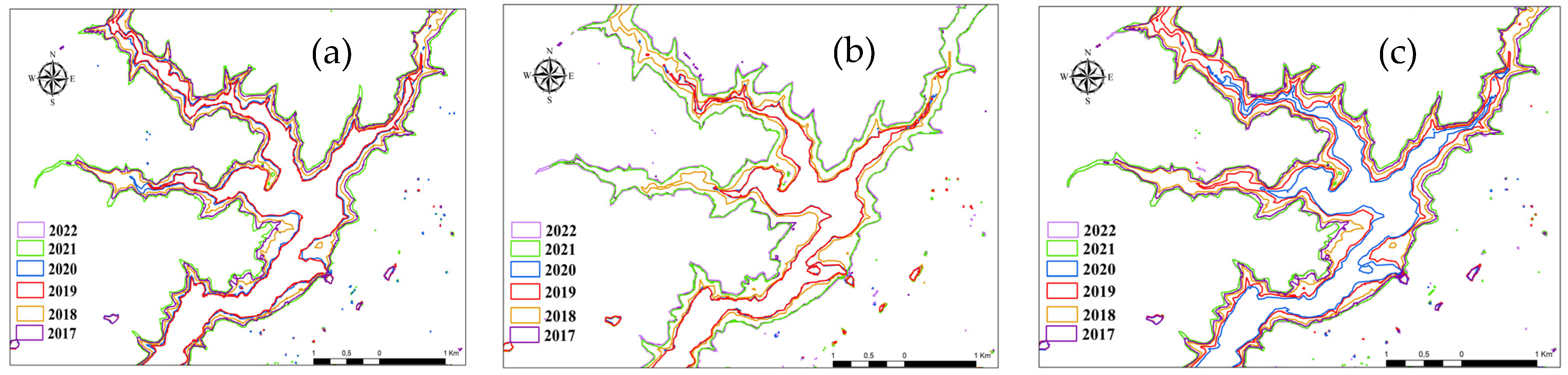
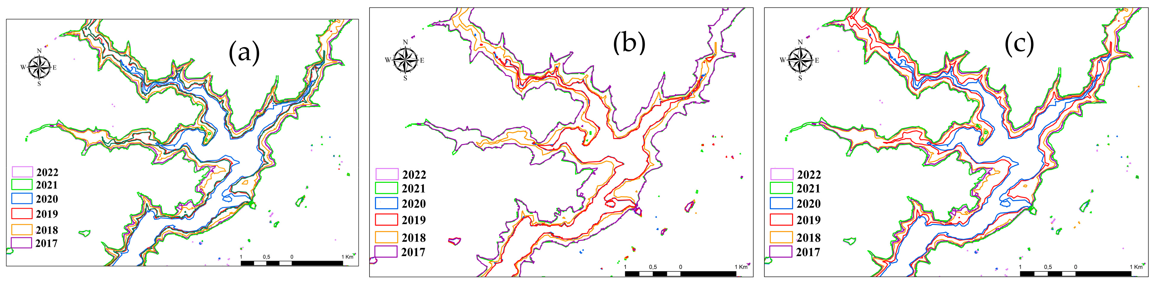
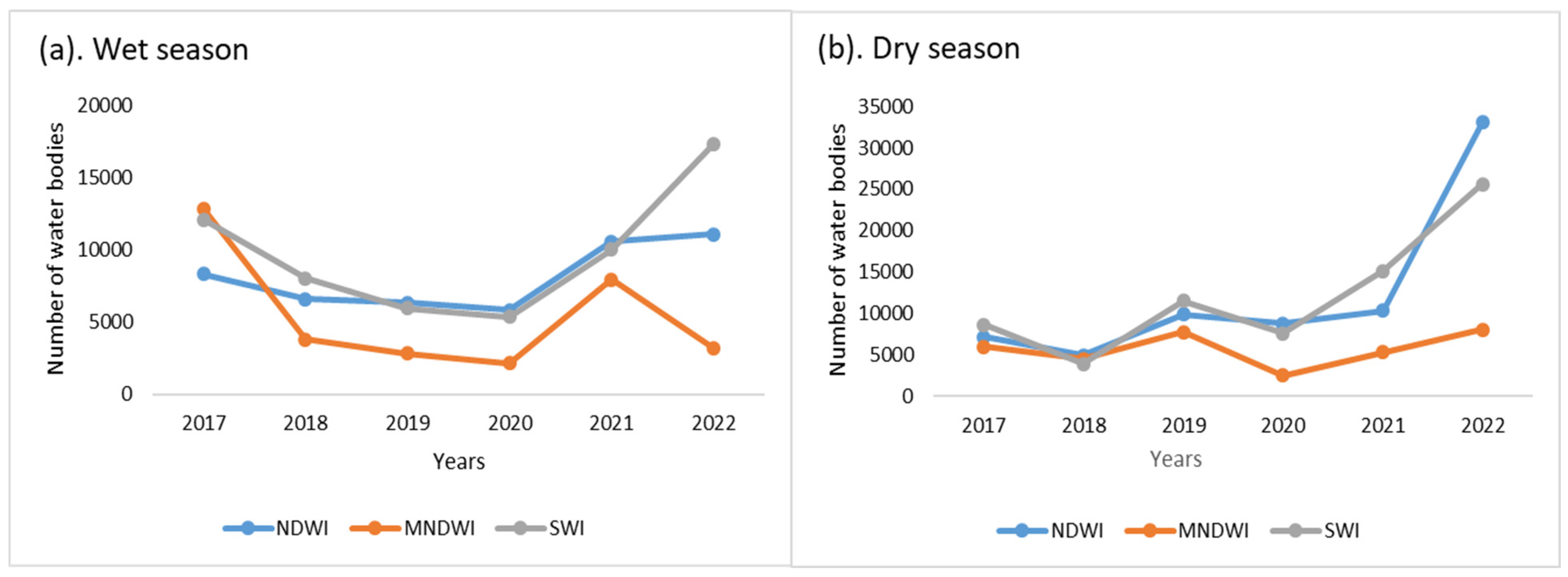
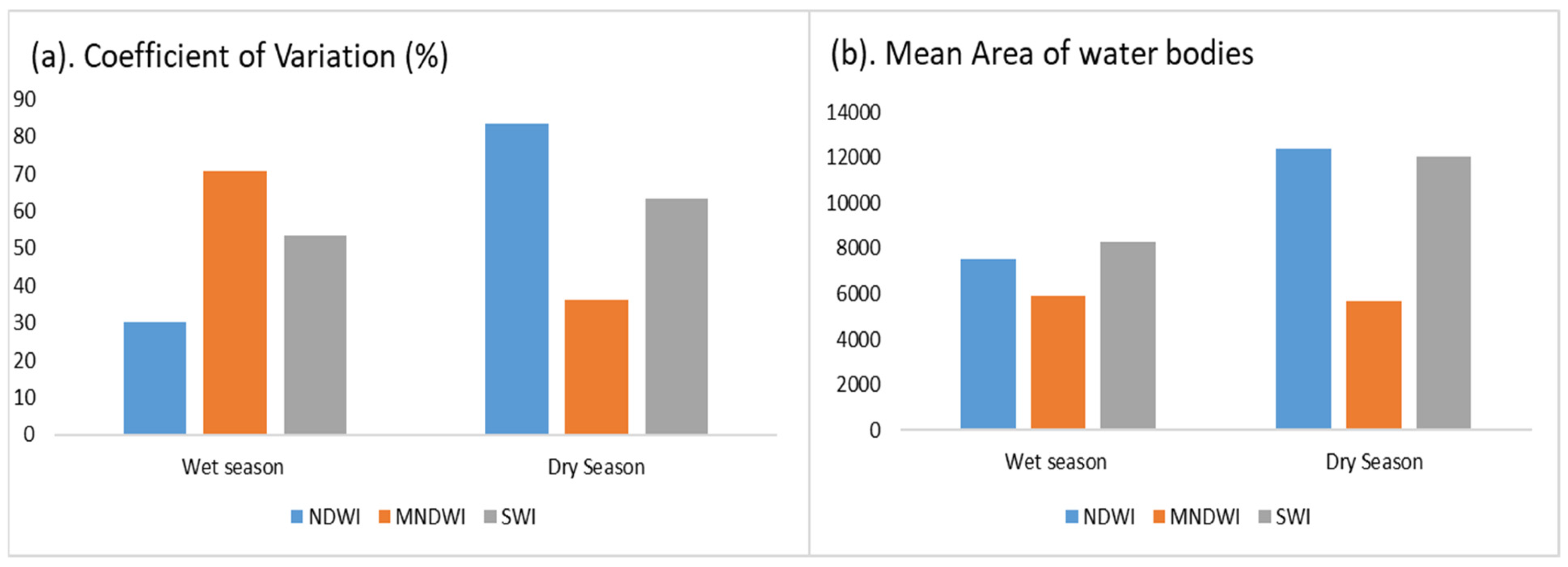
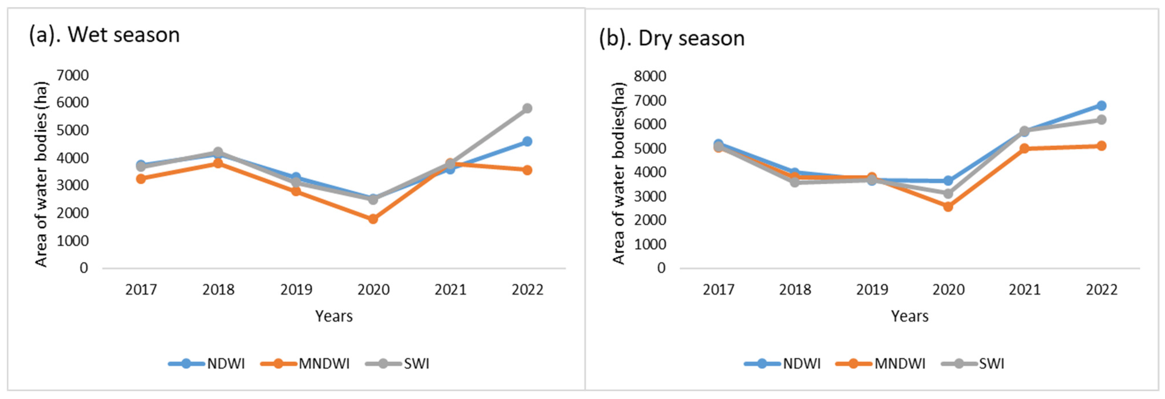
3.2. Intra and Inter-Seasonal Dynamics of Surface Water Bodies

The Letaba catchment exhibited varying numbers of water bodies extracted through the spectral water indices. For example, the minimum count was 2514 for the MNDWI in 2020, while other indices such as the NDWI and SWI recorded 4948 and 3922, respectively, during the 2018 wet season. Notably, the highest number of water bodies was observed in 2022 during the wet season, with 8022 for the MNDWI, 28,973 for the NDWI, and 25,594 for the SWI (Figure 4a,b).

During the dry season, the minimum number of water bodies ranged from 2124 for the MNDWI in 2020 to 5527 for the NDWI and 7649 for the SWI in 2017. In contrast, the maximum counts during this period reached 8022 for the MNDWI, 25,594 for the SWI, and 33,029 for the NDWI in 2022 (as shown in Figure 4a,b). The number of water bodies exhibited notable seasonal variations, with higher counts during the dry season when more surface water was present in the landscape, and lower counts during the wet season when fewer water bodies were observed.

Furthermore, the average size of the water bodies varied, with larger sizes observed during the dry season and smaller sizes during the wet season. This indicates that water bodies were more diverse in size during the dry season, whereas they were generally larger in the wet season. The trend is further illustrated in the results (Figure 5b), where a greater number of water bodies is observed in the dry season compared to the wet season.

In terms of the total area covered by water bodies, the landscape exhibited a range, from a minimum of 1795 to 2527 ha during the wet season and from 2592 to 6809 ha during the dry season across different years (Figure 6a,b). Both seasons exhibited variability in terms of both the number and size of water bodies. Notably, there was a gradual increase in the number of water bodies during the dry season starting from 2019, with a decline observed in 2018. The mean area of water bodies also increased during the dry season. All four landscape metrics demonstrated both intra and inter-seasonal changes in the distribution of surface water bodies.

4. Discussion

This work aimed to test the utility of integrating spectral indices obtained from Sentinel 2 imagery with landscape metrics to map the spatial and seasonal fluctuations in surface water bodies within the Letaba catchment, which is situated in tropical semi-arid southern Africa. The geospatial analysis was conducted using GEE, and although certain months presented difficulties in obtaining cloud-free images, GEE’s approach of consolidating images from the different months into a single stack proved to be advantageous. This method effectively reduced the proportion of the area covered by clouds and offered a solution to the challenge of cloud-free imagery. Although GEE was effective in monitoring water bodies in the Letaba catchment, there are limitations associated with the cloud computing platform. The limitations of GEE include the spatial and temporal resolutions of the satellite images, which may not be adequate for capturing fine-scale changes in a heterogeneous landscape. Cloud cover can be a significant issue in tropical regions; this can limit the availability of cloud-free imagery, which affects the temporal consistency and reliability of detecting changes in water bodies [38].

Sentinel-2 has proven to be an effective tool for detecting and mapping water bodies in the Letaba catchment. Its advantages include the ability to capture imagery at regular intervals, enabling the near-real-time monitoring of changes in water bodies, and facilitating accurate water body detection [39]. Moreover, Sentinel-2′s wide swath coverage helps capture large areas efficiently, making it suitable for assessing the extent of water bodies in the Letaba catchment. However, there are several challenges associated with using Sentinel-2 for this purpose. One major challenge is the influence of cloud cover on data acquisition. In regions like the Letaba catchment, which may experience frequent cloud cover, obtaining cloud-free imagery can be difficult, leading to data gaps and hindering our ability to monitor water bodies consistently. However, studies [40,41] have shown that synthetic aperture radars (SARs) are able to deal with clouds since they are not affected by clouds.

The accomplishment of consistently high overall accuracy levels, ranging from 96% to a perfect 100% over the five-year period in both wet and dry seasons (2017–2022), in the detection and mapping of water bodies within the Letaba catchment using the Sentinel-2-derived spectral indices NDWI, SWI and MNDWI is remarkable (Table 3). These results align with previous studies that have highlighted the reliability of spectral indices in water body delineation [6,35]. This high accuracy suggests that despite the known limitations of individual indices, their application in this study is robust across varying hydrological conditions.

Our success in maintaining high levels of accuracy across different seasons underscores the adaptability of these indices in detecting water bodies under dynamic environmental conditions. The NDWI and SWI, with their strong sensitivity to the presence of water, have likely contributed to the stability of these results, while the MNDWI, despite its lower sensitivity to certain water types, has provided additional value in distinguishing water from built-up and vegetated areas [27].

Furthermore, the classification results demonstrate a high level of accuracy, indicating strong agreement between the water indices outputs and ground-truth data. This high accuracy reflects the indices’ ability to effectively differentiate water and non-water bodies across various environmental conditions from 2017 to 2022. A key factor contributing to this performance is the high True Positive (TP) and True Negative (TN) rates, which indicate that both water bodies and non-water bodies were correctly classified with minimal errors. The low False Positive (FP) and False Negative (FN) values further validate the robustness of the classification method by minimizing misclassification. This study aligns with the findings of [36], which emphasize the necessity of robust validation frameworks in remote sensing-based water classification.

The significance of these findings cannot be understated, as they have direct implications for water resource management, land-use planning, and ecological conservation in the region, particularly in an area like Letaba where seasonal fluctuations in water availability can be significant. However, it is essential to look deeper into the factors contributing to the variations observed within the accuracy range, which could be influenced by seasonal changes, water quality dynamics, or even differences in the image acquisition conditions [6,42]. Additionally, the study’s validation and ground-truthing efforts should be discussed to provide a comprehensive understanding of the accuracy assessment’s credibility. The sustained high accuracy in mapping water bodies using the NDWI, SWI and MNDWI throughout both wet and dry seasons in the Letaba catchment demonstrates the robustness of the chosen methodology and its potential to address critical water-related challenges in the region across different climatic conditions. Similar results were obtained in a study by [18], which stipulated the effectiveness of spectral indices derived from Sentinel 2 in extracting water bodies in China.

The application of landscape metrics integrated with the accuracy and precision of derived spectral indices is important for the effective management of water resources in tropical semi-arid environments. The total number of water bodies showed high seasonality, with a high number of water bodies in the dry season and a lower number in the wet season in the study area. Although the areas receive much rainfall during the wet season, the study observed a lower number of water bodies. This could be attributed to the high temperatures in this season, which dry up the landscape. The increased number of water bodies in the dry season could be attributed to a number of constructed dams or reservoirs that are found within the catchment, and this was confirmed by the Department of Water Affairs and Forestry [27]. The increasing number of water bodies from 2021 to 2022 could be due to high rainfall. Similar results were obtained by [43], who observed an increasing number of water bodies from 2000 to 2020 with increased rainfall. Conversely, in 2020, there was a decrease in surface water bodies within the study area in both the dry and wet seasons. This may be because of the lower rainfall received by the area. The average number of water bodies was associated with a coefficient of variation of 87%, 36% and 63% for the NDWI, MNDWI, and SWI, respectively, in the dry season. The study’s coefficient of variation (CV) results reveals distinct seasonal variability in the water indices. During the wet season, the NDWI exhibited low variability (30%), indicating the stable presence of water, the MNDWI showed high variability (70%), likely due to land cover influences and mixed water signals, and the SWI had moderate variability (50%), reflecting fluctuations in surface moisture. In the dry season, the NDWI’s variability sharply increased to 80%, suggesting significant seasonal water loss, whereas the MNDWI’s CV dropped to 30%, indicating stability in detecting the remaining water bodies. The SWI’s variability increased to 60%, highlighting changes in the extent of surface water and soil moisture retention. These findings emphasize the importance of using multiple indices to capture seasonal hydrological changes, providing valuable insights for water resource management and climate adaptation strategies.

Despite this, all these water indices were able detect water within the study area. The study also observed that the MNDWI detected fewer water bodies, especially during the wet season. The MNDWI is particularly effective in detecting water in areas where the presence of vegetation or urban features could otherwise obscure water bodies when using other indices like the NDWI or SWI. A key reason for the observed differences is that the MNDWI is highly sensitive to built-up areas and certain types of vegetation, which can introduce commission errors, leading to a lower user accuracy (UA). However, even with a UA of approximately 80%, the MNDWI still provides robust results when identifying water bodies. This is particularly important given the challenges associated with detecting water in heterogeneous landscapes where spectral mixing occurs, where other indices may overestimate or misclassify water bodies. The ability of the MNDWI to distinguish between water and non-water surfaces in such areas can enhance the overall accuracy of water mapping efforts. Although the MNDWI may yield a smaller total water area, it provides critical information about the presence of water in regions where other indices might fail. Therefore, including the MNDWI in water body detection maps adds robustness to the analysis, as it can help identify water bodies that may not be detected by other indices, ultimately improving the comprehensiveness of water mapping.

Additionally, the lower mean water area in Figure 4b and the lower total water area in Figure 5 (particularly in the wet season of 2022) can be attributed to variations in the surface reflectance, caused by seasonal changes, water turbidity, and shadowing effects. This limitation was more evident during wet seasons, particularly in 2022, when increased precipitation led to more sediment-laden or vegetation-covered water surfaces that the MNDWI struggled to detect. However, when considering its overall performance across different conditions, the MNDWI remains effective for water body mapping. In practical applications, stacking images and cross-validation with multiple indices help mitigate these discrepancies. For instance, studies have shown that combining the MNDWI with other indices, such as the NDWI and AWEI, improves the overall classification accuracy in diverse landscapes [44,45,46]. Despite its slightly lower UA compared to other indices, the MNDWI remains a valuable tool in water body detection, particularly in areas with complex land cover interactions.

This study also recommends integrating riverine systems into surface water assessments as a valuable direction for future research. This approach enhances our understanding of hydrological dynamics, improves water resource management, and supports sustainable decision-making. By incorporating riverine interactions, researchers can better assess water availability, quality, and resilience in the face of climate change and increasing human demands.

5. Conclusions

This study of the Letaba catchment revealed a significant variability in water bodies within this semi-arid tropical environment, emphasizing the effectiveness of Sentinel-2-derived spectral indices (NDWI, SWI, and MNDWI) in seasonal water body monitoring. By leveraging GEE, large-scale data processing was efficiently conducted, allowing for the detection and analysis of spatial and temporal water body dynamics. The integration of landscape metrics further enhanced the assessment by providing insights into the distribution, extent, and connectivity of surface water over time. The findings indicate notable seasonal variation, with the dry season exhibiting a higher number and larger area of water bodies compared to the wet season. This unexpected trend highlights the complex hydrological interactions within the catchment and underscores the need for continuous monitoring to accurately capture these fluctuations. A rigorous validation and ground-truthing process, incorporating a confusion matrix and key accuracy metrics (TP, TN, FP, and FN), confirmed the high classification accuracy (96–100%). The strong agreement between the classification results and reference data reinforces the credibility of remote sensing-based methods for water body assessment. This level of accuracy ensures that the extracted water body information is reliable for hydrological modeling, resource management, and climate adaptation planning.

These findings highlight the critical role of remote sensing and geospatial technologies in supporting water management strategies. By providing high-precision, real-time data, this study offers actionable insights for policymakers and stakeholders to enhance water allocation, conservation, and sustainable use in the Letaba catchment and other regions facing similar climatic challenges. Ensuring water security, supporting agriculture, and maintaining ecosystem resilience requires an adaptive approach, and these results contribute to improving long-term water resource sustainability.

Furthermore, this study demonstrates the potential of integrating cloud-based geospatial analysis (GEE) with landscape metrics and high-resolution Sentinel-2 imagery to develop scalable, data-driven solutions for monitoring and managing water resources under changing climate conditions. This approach strengthens the foundation for more resilient and adaptive water management strategies, ensuring sustainable resource availability in semi-arid tropical landscapes facing increasing water scarcity.

References

1. Rokni, K.; Ahmad, A.; Solaimani, K.; Hazini, S. A new approach for surface water change detection: Integration of pixel level image fusion and image classification techniques. Int. J. Appl. Earth Obs. Geoinf. 2015, 34, 226–234. [Google Scholar] [CrossRef]
2. Khalid, H.W.; Khalil, R.M.Z.; Qureshi, M.A. Evaluating spectral indices for water bodies extraction in western Tibetan Plateau. Egypt. J. Remote Sens. Space Sci. 2021, 24, 619–634. [Google Scholar] [CrossRef]
3. Verpoorter, C.; Kutser, T.; Tranvik, L. Automated mapping of water bodies using Landsat multispectral data. Limnol. Oceanogr. Methods 2012, 10, 1037–1050. [Google Scholar]
4. Collet, L.; Ruelland, D.; Borrell-Estupina, V.; Servat, E. Assessing the long-term impact of climatic variability and human activities on the water resources of a meso-scale Mediterranean catchment. Hydrol. Sci. J. 2014, 59, 1457–1469. [Google Scholar]
5. Haas, E.M.; Bartholomé, E.; Combal, B. Time series analysis of optical remote sensing data for the mapping of temporary surface water bodies in sub-Saharan western Africa. J. Hydrol. 2009, 370, 52–63. [Google Scholar] [CrossRef]
6. Feyisa, G.L.; Meilby, H.; Fensholt, R.; Proud, S.R. Automated Water Extraction Index: A new technique for surface water mapping using Landsat imagery. Remote Sens. Environ. 2014, 140, 23–35. [Google Scholar] [CrossRef]
7. Tulbure, M.G.; Broich, M. Spatiotemporal dynamic of surface water bodies using Landsat time-series data from 1999 to 2011. ISPRS J. Photogramm. Remote Sens. 2013, 79, 44–52. [Google Scholar] [CrossRef]
8. Gan, R.; Zhang, Y.; Shi, H.; Yang, Y.; Eamus, D.; Cheng, L.; Chiew, F.H.; Yu, Q. Use of satellite leaf area index estimating evapotranspiration and gross assimilation for Australian ecosystems. Ecohydrology 2018, 11, e1974. [Google Scholar]
9. Kusangaya, S.; Warburton, M.L.; Van Garderen, E.A.; Jewitt, G.P. Impacts of climate change on water resources in southern Africa: A review. Phys. Chem. Earth 2014, 67, 47–54. [Google Scholar]
10. Bhangale, U.; More, S.; Shaikh, T.; Patil, S.; More, N. Analysis of surface water resources using Sentinel-2 imagery. Procedia Comput. Sci. 2020, 171, 2645–2654. [Google Scholar]
11. Klein, I.; Dietz, A.J.; Gessner, U.; Galayeva, A.; Myrzakhmetov, A.; Kuenzer, C. Evaluation of seasonal water body extents in Central Asia over the past 27 years derived from medium-resolution remote sensing data. Int. J. Appl. Earth Obs. Geoinf. 2014, 26, 335–349. [Google Scholar] [CrossRef]
12. Zou, Z.; Dong, J.; Menarguez, M.A.; Xiao, X.; Qin, Y.; Doughty, R.B.; Hooker, K.V.; Hambright, K.D. Continued decrease of open surface water body area in Oklahoma during 1984–2015. Sci. Total Environ. 2017, 595, 451–460. [Google Scholar] [PubMed]
13. Sarp, G.; Ozcelik, M. Water body extraction and change detection using time series: A case study of Lake Burdur, Turkey. J. Taibah Univ. Sci. 2017, 11, 381–391. [Google Scholar] [CrossRef]
14. Khandelwal, A.; Karpatne, A.; Marlier, M.E.; Kim, J.; Lettenmaier, D.P.; Kumar, V. An approach for global monitoring of surface water extent variations in reservoirs using MODIS data. Remote Sens. Environ. 2017, 202, 113–128. [Google Scholar] [CrossRef]
15. Pickens, A.H.; Hansen, M.C.; Hancher, M.; Stehman, S.V.; Tyukavina, A.; Potapov, P.; Marroquin, B.; Sherani, Z. Mapping and sampling to characterize global inland water dynamics from 1999 to 2018 with full Landsat time-series. Remote Sens. Environ. 2020, 243, 111792. [Google Scholar]
16. Fisher, A.; Flood, N.; Danaher, T. Comparing Landsat water index methods for automated water classification in eastern Australia. Remote Sens. Environ. 2016, 175, 167–182. [Google Scholar] [CrossRef]
17. Mashala, M.J.; Dube, T.; Mudereri, B.T.; Ayisi, K.K.; Ramudzuli, M.R. A Systematic Review on Advancements in Remote Sensing for Assessing and Monitoring Land Use and Land Cover Changes Impacts on Surface Water Resources in Semi-Arid Tropical Environments. Remote Sens. 2023, 15, 3926. [Google Scholar] [CrossRef]
18. Jiang, W.; Ni, Y.; Pang, Z.; Li, X.; Ju, H.; He, G.; Lv, J.; Yang, K.; Fu, J.; Qin, X. An effective water body extraction method with new water index for sentinel-2 imagery. Water 2021, 13, 1647. [Google Scholar] [CrossRef]
19. Yang, X.; Zhao, S.; Qin, X.; Zhao, N.; Liang, L. Mapping of urban surface water bodies from Sentinel-2 MSI imagery at 10 m resolution via NDWI-based image sharpening. Remote Sens. 2017, 9, 596. [Google Scholar] [CrossRef]
20. Mashala, M.J.; Dube, T.; Ayisi, K.K.; Ramudzuli, M.R. Using the Google Earth Engine cloud-computing platform to assess the long-term spatial temporal dynamics of land use and land cover within the Letaba watershed, South Africa. Geocarto Int. 2023, 38, 2252781. [Google Scholar] [CrossRef]
21. Shafizadeh-Moghadam, H.; Khazaei, M.; Alavipanah, S.K.; Weng, Q. Google Earth Engine for large-scale land use and land cover mapping: An object-based classification approach using spectral, textural and topographical factors. GIScience Remote Sens. 2021, 58, 914–928. [Google Scholar]
22. Sherjah, P.Y.; Sajikumar, N.; Nowshaja, P.T. Quality monitoring of inland water bodies using Google Earth Engine. J. Hydroinformatics 2023, 25, 432–450. [Google Scholar]
23. Gujrati, A.; Jha, V.B. Surface water dynamics of inland water bodies of India using Google Earth Engine. ISPRS Ann. Photogramm. Remote Sens. Spat. Inf. Sci. 2018, 4, 467–472. [Google Scholar]
24. Nguyen, U.N.; Pham, L.T.; Dang, T.D. An automatic water detection approach using Landsat 8 OLI and Google Earth Engine cloud computing to map lakes and reservoirs in New Zealand. Environ. Monit. Assess. 2019, 191, 235. [Google Scholar]
25. Frazier, A.E.; Kedron, P. Landscape metrics: Past progress and future directions. Curr. Landsc. Ecol. Rep. 2017, 2, 63–72. [Google Scholar]
26. Walz, U. Landscape structure, landscape metrics and biodiversity. Living Rev. Landsc. Res. 2011, 5, 1–35. [Google Scholar]
27. DWAF. Letaba Catchment Reserve Determination Study; February 2006; Department of Water Affairs and Forestry: Pretoria, South Africa, 2006. [Google Scholar]
28. Tucker, C.J. Red and photographicinfrared linear combinations for monitoring vegetation. Remote Sens. Environ. 1979, 8, 127–150. [Google Scholar]
29. Gao, B.C. Normalized difference water index for remote sensing of vegetation liquid water from space. In Proceedings of the SPIE’S 1995 Symposium on OE/Aerospace Sensing and Dual Use Photonics, Orlando, FL, USA, 17–21 April 1995; pp. 225–236. [Google Scholar] [CrossRef]
30. Acharya, T.D.; Subedi, A.; Lee, D.H. Evaluation of water indices for surface water extraction in a Landsat 8 scene of Nepal. Sensors 2018, 18, 2580. [Google Scholar] [CrossRef]
31. Zhai, K.; Wu, X.; Qin, Y.; Du, P. Comparison of surface water extraction performances of different classic water indices using OLI and TM imageries in different situations. Geo-Spat. Inf. Sci. 2015, 18, 32–42. [Google Scholar] [CrossRef]
32. Zhou, Y.; Dong, J.; Xiao, X.; Xiao, T.; Yang, Z.; Zhao, G.; Zou, Z.; Qin, Y. Open surface water mapping algorithms: A comparison of water-related spectral indices and sensors. Water 2017, 9, 256. [Google Scholar] [CrossRef]
33. Șerban, C.; Maftei, C.; Dobrică, G. Surface water change detection via water indices and predictive modeling using remote sensing imagery: A case study of Nuntasi-Tuzla Lake, Romania. Water 2022, 14, 556. [Google Scholar] [CrossRef]
34. McFeeters, S.K. The use of the Normalized Difference Water Index (NDWI) in the delineation of open water features. Int. J. Remote Sens. 1996, 17, 1425–1432. [Google Scholar]
35. Xu, H. Modification of normalised difference water index (NDWI) to enhance open water features in remotely sensed imagery. Int. J. Remote Sens. 2006, 27, 3025–3033. [Google Scholar]
36. Albarqouni, M.M. Yagmur, N. Bektas Balcik, F.; Sekertekin, A. Assessment of Spatio-Temporal Changes in Water Surface Extents and Lake Surface Temperatures Using Google Earth Engine for Lakes Region, Türkiye. ISPRS Int. J. Geo-Inf. 2022, 11, 407. [Google Scholar] [CrossRef]
37. Yesuph, A.Y.; Dagnew, A.B. Land use/cover spatiotemporal dynamics, driving forces and implications at the Beshillo catchment of the Blue Nile Basin, North Eastern Highlands of Ethiopia. Environ. Syst. Res. 2019, 8, 21. [Google Scholar]
38. Kandekar, V.U.; Pande, C.B.; Rajesh, J.; Atre, A.A.; Gorantiwar, S.D.; Kadam, S.A.; Gavit, B. Surface water dynamics analysis based on sentinel imagery and Google Earth Engine Platform: A case study of Jayakwadi dam. Sustain. Water Resour. Manag. 2021, 7, 44. [Google Scholar]
39. Lombana, L.; Martínez-Graña, A. A Flood Mapping Method for Land Use Management in Small-Size Water Bodies: Validation of Spectral Indexes and a Machine Learning Technique. Agronomy 2022, 12, 1280. [Google Scholar] [CrossRef]
40. Marzi, D.; Gamba, P. Inland water body mapping using multitemporal sentinel-1 sar data. IEEE J. Sel. Top. Appl. Earth Obs. Remote Sens. 2021, 14, 11789–11799. [Google Scholar]
41. Musa, Z.N.; Popescu, I.; Mynett, A. A review of applications of satellite SAR, optical, altimetry and DEM data for surface water modelling, mapping and parameter estimation. Hydrol. Earth Syst. Sci. 2015, 19, 3755–3769. [Google Scholar]
42. Wu, F.; Yang, X.; Cui, Z.; Ren, L.; Jiang, S.; Liu, Y.; Yuan, S. The impact of human activities on blue-green water resources and quantification of water resource scarcity in the Yangtze River Basin. Sci. Total Environ. 2024, 909, 168550. [Google Scholar]
43. Anusha, B.N.; Babu, K.R.; Kumar, B.P.; Kumar, P.R.; Rajasekhar, M. Geospatial approaches for monitoring and mapping of water resources in semi-arid regions of Southern India. Environ. Chall. 2022, 8, 100569. [Google Scholar]
44. Laonamsai, J.; Julphunthong, P.; Saprathet, T.; Kimmany, B.; Ganchanasuragit, T.; Chomcheawchan, P.; Tomun, N. Utilizing NDWI, MNDWI, SAVI, WRI, and AWEI for estimating erosion and deposition in Ping River in Thailand. Hydrology 2023, 10, 70. [Google Scholar] [CrossRef]
45. Masocha, M.; Dube, T.; Makore, M.; Shekede, M.D.; Funani, J. Surface water bodies mapping in Zimbabwe using landsat 8 OLI multispectral imagery: A comparison of multiple water indices. Phys. Chem. Earth Parts A/B/C 2018, 106, 63–67. [Google Scholar] [CrossRef]
46. Rajeswari, S.; Rathika, P. Exploring Spectral Indices for Improved Water Body Classification in Landsat Imagery. In Proceedings of the 2024 Third International Conference on Intelligent Techniques in Control, Optimization and Signal Processing (INCOS), Virudhunagar, India, 14–16 March 2024; pp. 1–5. [Google Scholar]
Figure 1. Location of the Letaba watershed, South Africa.
Hydrology 12 00068 g001
Figure 2. Extracted water bodies using (a) NDWI, (b) MNDWI, and (c) SWI in the dry season.
Hydrology 12 00068 g002
Figure 3. Extracted surface water bodies using (a) NDWI, (b) MNDWI, and (c) SWI in the wet season.
Hydrology 12 00068 g003
Figure 4. The number of water bodies within a landscape in (a) the wet season and (b) dry season.
Hydrology 12 00068 g004
Figure 5. (a) Coefficient of variation for the mean area of the number of water bodies within the landscape and (b) average area of water bodies in a landscape.
Hydrology 12 00068 g005
Figure 6. Total area of water bodies in (a) wet season and (b) dry season within the landscape from 2017 to 2022.
Hydrology 12 00068 g006