Spatio-Temporal Graph Neural Networks for Streamflow Prediction in the Upper Colorado Basin

Abstract

Streamflow prediction is vital for effective water resource management, enabling a better understanding of hydrological variability and its response to environmental factors. This study presents a spatio-temporal graph neural network (STGNN) model for streamflow prediction in the Upper Colorado River Basin (UCRB), integrating graph convolutional networks (GCNs) to model spatial connectivity and long short-term memory (LSTM) networks to capture temporal dynamics. Using 30 years of monthly streamflow data from 20 monitoring stations, the STGNN predicted streamflow over a 36-month horizon and was evaluated against traditional models, including random forest regression (RFR), LSTM, gated recurrent units (GRU), and seasonal auto-regressive integrated moving average (SARIMA). The STGNN outperformed these models across multiple metrics, achieving an R² of 0.78, an RMSE of 0.81 mm/month, and a KGE of 0.79 at critical locations like Lees Ferry. A sequential analysis of input–output configurations identified the (36, 36) setup as optimal for balancing historical context and forecasting accuracy. Additionally, the STGNN showed strong generalizability when applied to other locations within the UCRB. These results underscore the importance of integrating spatial dependencies and temporal dynamics in hydrological forecasting, offering a scalable and adaptable framework to improve predictive accuracy and support adaptive water resource management in river basins.

1. Introduction

Rivers are the lifeblood of human civilization, shaping landscapes, nurturing biodiversity, and supporting communities and industries. They serve as critical pathways within the global hydrological cycle, regulating regional water availability, influencing agricultural productivity, and maintaining ecosystem health. Rivers and their water systems face mounting challenges such as rapid population growth, land-use changes, expanding infrastructure, and, most critically, the effects of shifting environmental conditions [1,2,3]. As hydroclimatic regimes become more variable and extreme, understanding and predicting streamflow is essential for adaptively managing resources, mitigating flood risks, planning hydropower generation, and preserving ecological integrity [4,5,6,7,8].

Conventional hydrological modeling approaches, ranging from conceptual frameworks to physically based distributed models, have long been used to simulate the rainfall-runoff processes underlying streamflow [9,10,11]. Although these models have enhanced our understanding of watershed processes, their complexity, heavy parameterization requirements, and reliance on simplifying assumptions often limit their adaptability to non-stationary climate conditions [6,12,13,14]. Large-scale studies have also revealed long-term trends and variations in global and regional streamflow regimes, challenging traditional modeling paradigms [1,2,15]. Meanwhile, technological advances in remote sensing and data assimilation have enabled more comprehensive and accurate characterization of hydrological processes, driving the need for flexible, data-driven forecasting methods [4,16,17,18,19].

Over the past decade, data-driven and machine learning (ML) methods have emerged as powerful tools in hydrological forecasting. Techniques such as artificial neural networks (ANNs), support vector machines (SVMs), and recurrent neural networks (RNNs), including long short-term memory (LSTM) and gated recurrent unit (GRU) models, have shown promise in capturing complex, nonlinear hydrological dynamics without relying on strict physical assumptions [14,20,21,22,23,24,25,26,27]. These methods have improved short- to medium-term flow predictions, enhanced drought management strategies [28], and integrated climate teleconnections for extended lead-time forecasting [7,22,29]. However, many existing ML models often focus on temporal sequences at individual stations or treat spatially distributed inputs as fixed features, overlooking the rich spatial connectivity inherent in river basins [30,31]. A major breakthrough in ML-based hydrology is the integration of ensemble learning techniques, which combine multiple models to improve forecast reliability. An ensemble-based ML framework was proposed to enhance streamflow prediction by post-processing hydrological model outputs, demonstrating significant improvements in forecast accuracy [32]. Similarly, an ML-based flood forecasting system was introduced that integrates real-time hydrological data, highlighting the practical applicability of ML models in operational hydrological forecasting [33]. Despite these advancements, ML models often overlook spatial dependencies within river basins, limiting their ability to generalize predictions across diverse hydrological conditions. To address this issue, recent research has focused on graph-based neural networks, which explicitly model spatial relationships between different hydrological units [18,34].

Recognizing that hydrological processes are fundamentally spatial and interconnected, recent research has increasingly used graph neural networks (GNNs) to model river systems as networks of nodes (e.g., gauges, sub-basins) connected by edges representing river reaches and other hydrological pathways [18,35,36,37]. By adopting graph-based representations, GNNs inherently capture the structural information of watersheds, allowing upstream dynamics, catchment characteristics, and land surface properties to inform downstream predictions. When combined with advanced temporal modeling, spatio-temporal GNN frameworks have outperformed conventional ML methods in streamflow forecasting, demonstrating increased robustness under varying climatic and basin conditions [38,39,40,41]. These models have also integrated diverse data sources, such as meteorological variables, soil moisture, snowpack data, and climate indices, to improve predictive precision and relevance [31,42]. A physics-informed GNN model was developed to integrate river connectivity information into hydrological simulations, significantly enhancing forecast accuracy. This approach demonstrated that incorporating hydrological connectivity improves model generalization, particularly in ungauged basins [18]. Similarly, GNN applications across multiple U.S. basins have shown that graph-based hydrological models outperform traditional ML models by effectively leveraging spatial dependencies [34].

A key advancement in GNN-based hydrology is the development of spatio-temporal graph neural networks (STGNNs), which incorporate both spatial and temporal dependencies. The introduction of a Graph Transformer Network for flood forecasting demonstrated how graph-based architectures can enhance hydrological predictions by learning dynamic relationships across multiple timescales. The results showed a significant improvement in predicting flood events and extreme flow occurrences, highlighting the robustness of graph-based models in hydrological applications [43].

Despite the advantages of GNNs in capturing spatial dependencies, they often struggle with long-range temporal dependencies. To address this challenge, researchers have developed hybrid models that integrate GNNs with RNNs, LSTM networks, and Transformer architectures. A GNN-LSTM hybrid model applied for flood forecasting in the Mississippi River Basin demonstrated a significant reduction in RMSE compared to standard LSTMs, effectively capturing spatio-temporal dependencies for improved short-term flood prediction [44]. Similarly, a GCN-LSTM model used for streamflow prediction in the Yangtze River Basin showed enhanced accuracy for both dry and wet season forecasting [45]. These findings support the effectiveness of integrating graph-based learning with sequence modeling techniques to enhance streamflow forecasting capabilities. Moreover, studies on multi-basin streamflow forecasting using graph-based models indicate that hybrid GNN models generalize better across different hydrological regimes compared to purely data-driven models, emphasizing the importance of spatio-temporal learning architectures in improving hydrological predictions [34].

Although STGNNs and hybrid ML models offer superior performance in hydrological forecasting, they come with computational and scalability challenges. As the river network size increases, the computational burden grows significantly, leading to higher training times and potential overfitting [43]. Scaling GNNs to large hydrological networks requires efficient adjacency matrix construction and optimized graph convolutional operations [46]. Another key limitation is the need for high-quality hydrological datasets. Many river basins lack sufficient historical records, making it difficult to train data-driven models effectively [18]. To overcome these challenges, researchers have suggested the development of hybrid physics-informed ML models that integrate hydrological process knowledge with data-driven learning techniques to improve model generalization and accuracy.

Beyond streamflow forecasting, hydrological models also play a key role in reservoir operations and water resource management. Studies have emphasized the need to integrate advanced hydrological forecasting models into decision-support systems to optimize hydropower generation, irrigation, and flood control [47,48,49]. However, real-time reservoir operations are constrained by factors such as fluctuating power demand, hydrological uncertainties, storage levels, infrastructure limitations, and regulatory policies [50,51]. Traditional reservoir scheduling models often fail to capture dynamic operational constraints, necessitating the integration of AI-based hydropower scheduling techniques [52]. However, this study primarily focuses on improving streamflow forecasting accuracy across multiple stations, providing a fundamental input for operational decision making rather than directly modeling reservoir scheduling processes.

To address the limitations of existing approaches and improve streamflow forecasting, this study focuses on the following questions:

• Which ML approaches are most effective for streamflow forecasting across watersheds?
• How do the input and output sequence lengths influence the accuracy of predictions?
• Can the proposed machine learning model generalize to provide multistep runoff predictions across the entire watershed?

By addressing these questions, this study aims to advance data-driven hydrological modeling and provide reliable tools for streamflow forecasting, supporting adaptive water resource management in the face of an unpredictable climate and evolving environmental challenges. It seeks to empower hydrology stakeholders with an advanced awareness of streamflow patterns, enabling proactive decision making and improved resource planning.

2. Study Site

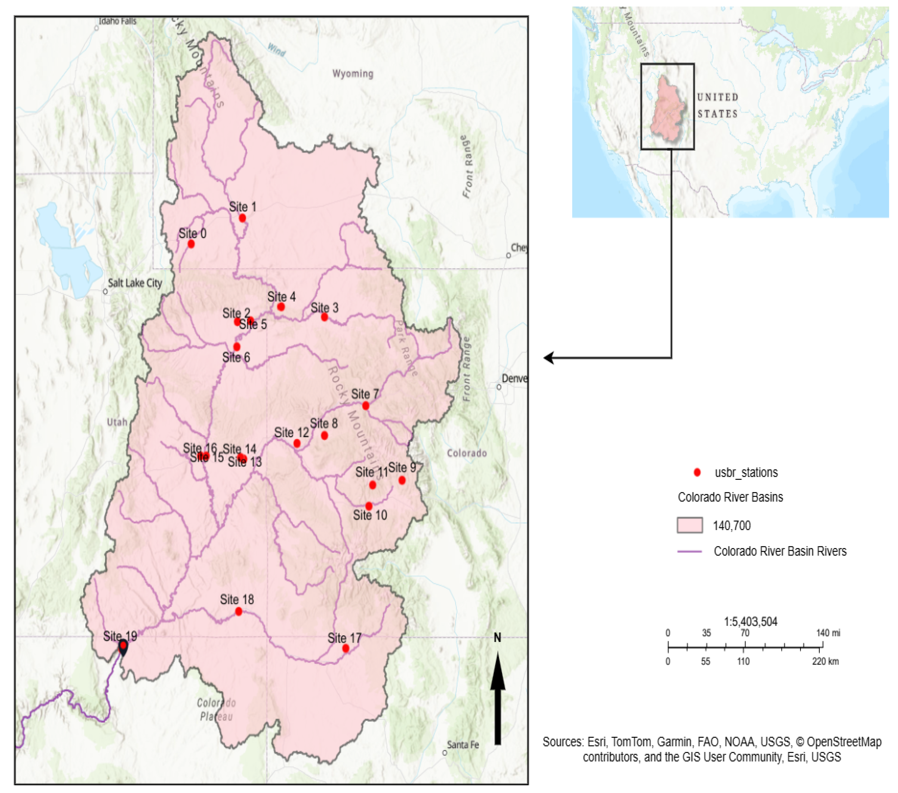
The Upper Colorado River Basin (UCRB) spans approximately 280,000 square kilometers and encompasses parts of Colorado, Utah, Wyoming, and New Mexico, with its outlet located at Lees Ferry, Arizona, as shown in Figure 1. The basin’s elevation ranges from 3300 m at its headwaters in the Rocky Mountains to 900 m near the Colorado–Utah state line [53,54].

The UCRB is a snowmelt-dominated hydrologic system, with approximately 70% of its annual runoff derived from high-elevation snowpack in the Rockies [55]. This snowmelt significantly influences the timing and magnitude of streamflows, which are critical to the region’s water supply. The primary stream in the UCRB is the Upper Colorado River, supported by major tributaries such as the Williams Fork, Blue River, Muddy Creek, Eagle River, Roaring Fork River, and Gunnison River.

Figure 1. Colorado River Basin with monitoring stations. Credit [56].

Figure 1. Colorado River Basin with monitoring stations. Credit [56].

The region’s hydrology is highly sensitive to climatic variations and changes in water storage, which significantly affect vegetation stability and water availability [4,5]. Streamflow prediction in the UCRB is particularly challenging due to its complex hydrological dynamics, influenced by variable snowmelt patterns, precipitation fluctuations, and evolving meteorological trends over time [1,2]. The UCRB’s significance extends beyond its immediate geographical boundaries, serving as a vital water source for the Lower Basin states, including Arizona, California, and Nevada [57].

The UCRB was selected as the study site due to its complex hydrological dynamics and the critical need for accurate streamflow forecasting. The basin is a highly regulated water system with multiple reservoirs and diversions, making it an ideal case study for evaluating data-driven modeling approaches. Additionally, the availability of long-term historical streamflow records and well-established monitoring networks makes it suitable for developing and validating machine learning-based forecasting models.

3. Data

Our research focuses on analyzing historical records of streamflow from the UCRB using data downloaded from the United States Bureau of Reclamation (USBR) website, accessible at (https://www.usbr.gov/lc/region/g4000/NaturalFlow/current.html), accessed on 9 August 2024. The dataset contains monthly river discharge measurements from 29 monitoring sites, covering a long-term historical period (1905–2023). We also collected geospatial data for the UCRB from the United States Geological Survey (USGS) ScienceBase catalog, website (https://www.sciencebase.gov/catalog/item/imap/4f4e4a38e4b07f02db61cebb), accessed on 9 August 2024. After mapping these monitoring station locations to the UCRB’s hydrological boundaries, only 20 stations were found to be relevant to the study. To ensure consistency across sites, streamflow values—initially reported in cubic feet per second (cfs) and acre-feet per month (ac-ft/month)—were standardized to millimeters per month (mm/month). This normalization process scales streamflow values to the basin’s hydrological characteristics, facilitating consistent analysis. Notable locations within this dataset include the Colorado River at Lees Ferry, AZ; the Yampa River near Maybell, CO; and the Colorado River below Parker Dam, AZ.

The USBR provides naturalized flow records adjusted to exclude anthropogenic influences such as reservoir operations and diversions. These flows are calculated using historical gauge measurements, hydrological modeling, and quality control protocols. Specifically, the USBR integrates USGS stream gauge data, precipitation, snowmelt, and land-use datasets to estimate unimpaired flow regimes while applying error-checking algorithms to ensure data consistency. Given the agency’s reputation in hydrological data curation, their quality assurance processes are considered robust. [58,59].

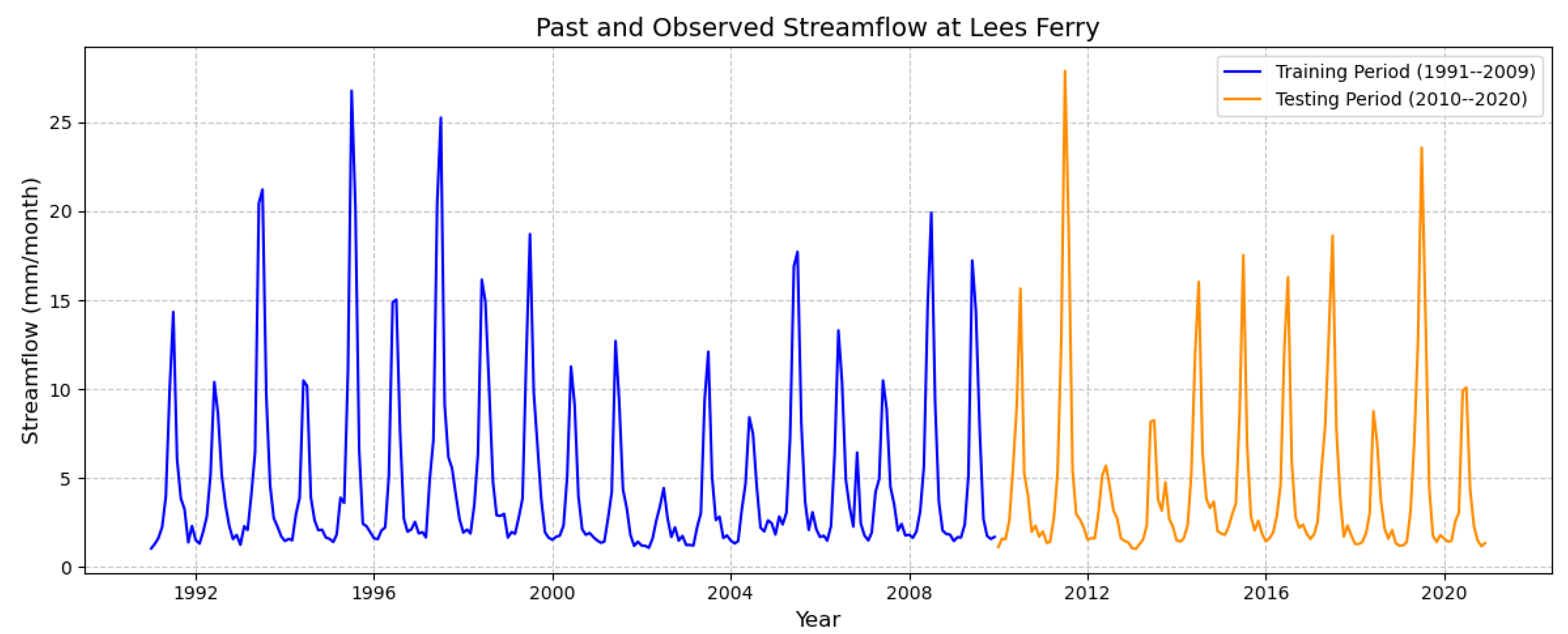
Our study focuses on a 30-year period, from 1991 to 2020. The dataset was divided into training and testing subsets, with 63.33% (January 1991 to December 2009) used for training and 36.67% (January 2010 to December 2020) reserved for testing. Figure 2 illustrates the raw streamflow data, highlighting distinct seasonal cycles and inter-annual variability. The training period (1991–2009) exhibits consistent periodic fluctuations, with annual peaks corresponding to the snowmelt runoff during spring and early summer. The testing period (2010–2020) shows a continuation of these seasonal patterns, although variations in magnitude suggest possible influences of climate variability and basin-specific hydrological responses. The clear seasonality observed in the raw data emphasizes the importance of incorporating temporal dependencies into predictive models.

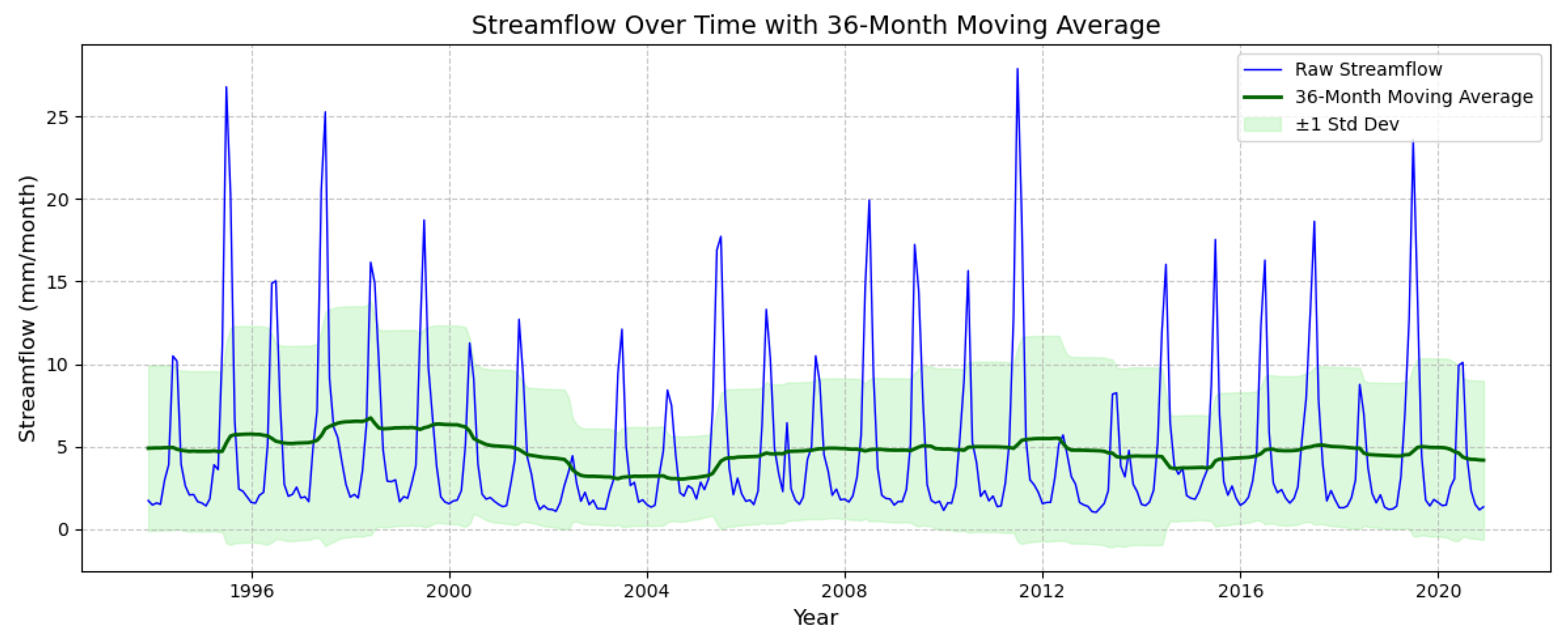
Figure 3 illustrates the temporal variation in streamflow (mm/month) from 1991 to 2020, incorporating both the raw monthly streamflow data (blue line) and a smoothed 36-month moving average (green line). Additionally, a shaded confidence band represents the ±1 standard deviation (light green), highlighting the variability in streamflow over time. The raw streamflow data exhibit pronounced seasonal peaks, primarily driven by hydrological events such as snowmelt and precipitation patterns. Variations in the peak magnitude indicate instances of extreme events, including potential floods or droughts. The 36-month moving average provides a clearer representation of long-term trends, showing a relatively stable baseline streamflow over the observed period.

Despite seasonal and inter-annual fluctuations, the long-term mean streamflow remains consistent, suggesting resilience in the hydrological system. However, the widening and contraction of the shaded standard deviation band indicate periods of increased variability, which could be linked to climatic shifts, land-use changes, or water management interventions. These variations underscore the importance of integrating long-term hydrological trends into predictive modeling to improve water resource management, mitigate flood risks, and enhance drought preparedness.

4. Methodology

This section provides an overview of the methodologies employed for streamflow forecasting.

4.1. Data Collection and Preprocessing

As described in Section 3, the dataset spans from 1991 to 2020 and includes standardized monthly streamflow measurements. No null or missing values were found in the collected data. The dataset was split into training and testing sets, with 63.33% of the data used for training and the remaining 36.67% reserved for testing. For modeling, the time series was divided into overlapping windows. Each window consisted of seq_len months of historical streamflow data, which were used to predict streamflow for the subsequent pred_len months:

$$X=[X_{t-\mathit{seq}\_\mathit{len}+1},X_{t-\mathit{seq}\_\mathit{len}+2},\dots ,X_t]$$

(1)

4.2. Random Forest Regression (RFR)

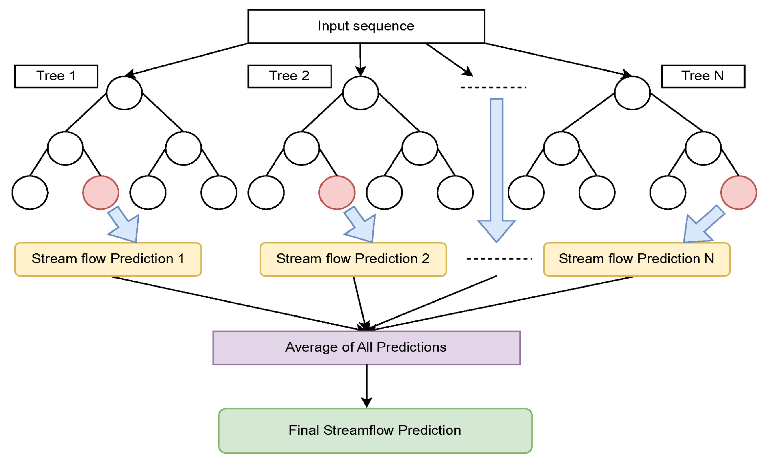
RFR is a tree-based induction model that combines predictions from multiple decision trees (DTs) to improve accuracy and reduce overfitting. Each tree in the forest is trained on different subsets of the dataset, and the final prediction is obtained by averaging the outputs of all the trees. This ensemble approach enhances predictive performance and robustness. Figure 4 illustrates a simplified structure of an RFR model, where each tree in the ensemble has a depth of 2, demonstrating how the predictions from individual trees contribute to the overall output. In general, RFR can be defined by the following equation:

$$\mathrm{RFR}\left(x\right)={\displaystyle \frac{1}{N}}\sum _{i=1}^N{T}_i\left(x\right)$$

(2)

where N is the number of decision trees, $T_i\left(x\right)$ is the prediction made by the i-th tree on input x, and $\mathrm{RFR}\left(x\right)$ represents the average prediction.

Figure 4. A simplified structure of RFR [60].

Figure 4. A simplified structure of RFR [60].

We performed hyperparameter tuning to develop the most effective models. For the univariate RFR, the best results were obtained using default hyperparameters, including 100 estimators, a minimum sample split of 2, a minimum sample leaf of 1, and the use of bootstrapping. Additionally, we explored various look-back window lengths to determine the most suitable configuration for optimal performance.

4.3. LSTM

RNNs are powerful tools for sequence modeling but encounter challenges with vanishing and exploding gradients when processing long sequences. These issues can hinder their ability to capture long-term dependencies. LSTM networks were developed to overcome these challenges, offering an effective solution for managing both short-term and long-term dependencies in sequential data [61,62]. LSTMs enhance the traditional RNN architecture by incorporating a memory cell and three distinct gates: the input gate, the forget gate, and the output gate. 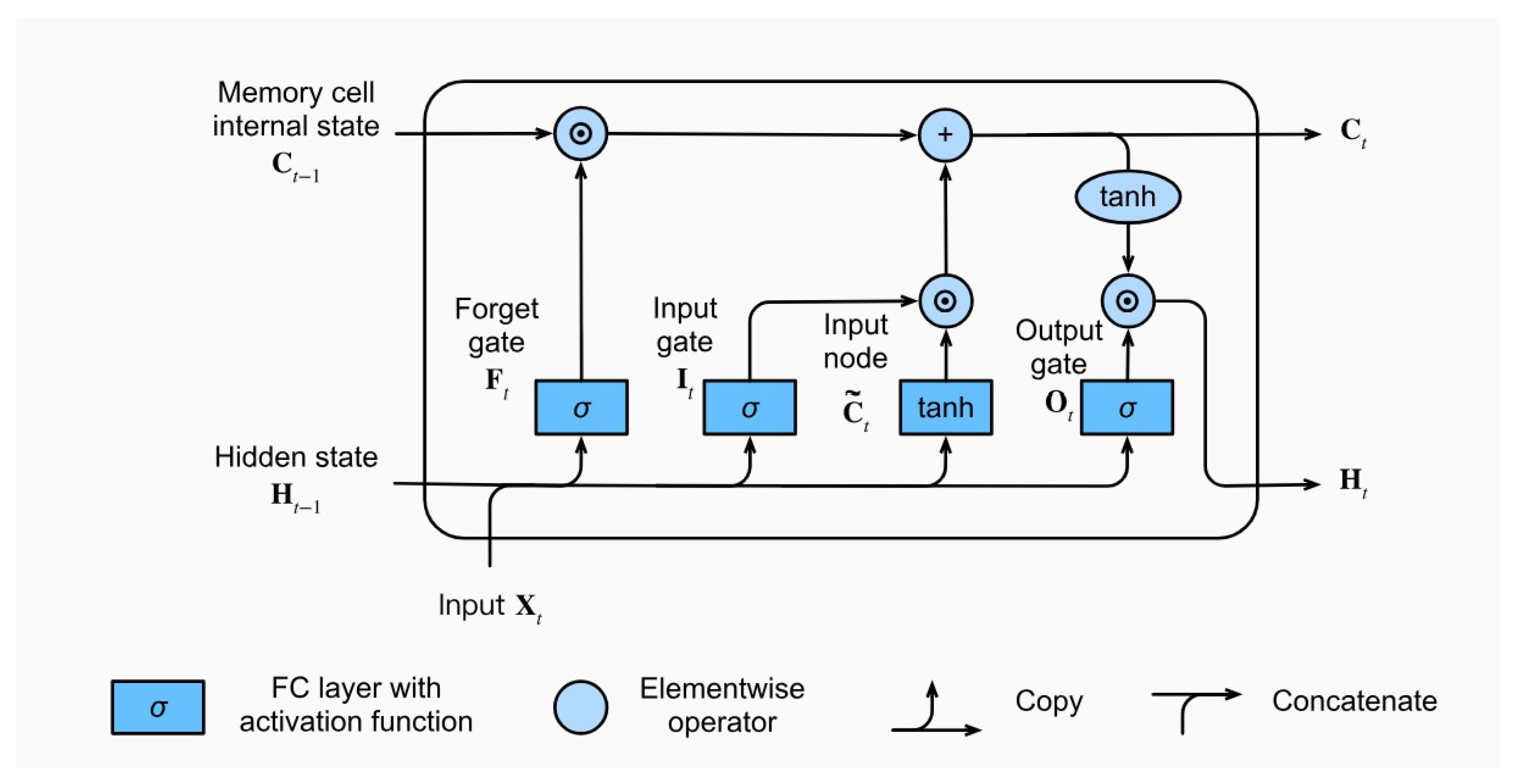These components collectively facilitate the retention and manipulation of information across extended sequences [63,64]. The LSTM architecture as illustrated in Figure 5 features a cell state that acts as a memory unit, enabling the retention of information over long sequences and addressing the limitations of traditional RNNs in capturing long-term dependencies [61,62]. This cell state plays a crucial role in maintaining relevant information over extended periods, which is vital for tasks requiring the retention of historical data. The following sections provide a detailed explanation of these gates and their mathematical formulations.

4.3.1. Input Gate

The input gate controls the flow of new information into the cell state. It uses a sigmoid activation function $\sigma$ to decide which parts of the input $x_t$ should be added to the cell state and a tanh activation function to generate candidate values for updating the cell state. Equation (3) defines the input gate input gate’s activation $i_t$.

$$i_t=\sigma (W_i·[h_{t-1},x_t]+b_i)$$

(3)

where $W_i$ represents the weight matrix for the input gate, $[h_{t-1},x_t]$ is the concatenation of the previous hidden state $h_{t-1}$ and the current input $x_t$, and $b_i$ is the bias term. The activation $i_t$ determines which parts of the new information are relevant to update the cell state at time step t.

4.3.2. Forget Gate

The forget gate determines which information from the previous cell state $c_{t-1}$ should be discarded. It also uses a sigmoid function to decide the extent of forgetting, effectively scaling the cell state values [65]. Equation (4) defines the forget gate’s activation $f_t$.

$$f_t=\sigma (W_f·[h_{t-1},x_t]+b_f)$$

(4)

where $W_f$ represents the weight matrix for the forget gate, $[h_{t-1},x_t]$ is the concatenation of the previous hidden state $h_{t-1}$ and the current input $x_t$, and $b_f$ is the bias term. The activation $f_t$ determines the proportion of information from the previous cell state $c_{t-1}$ that should be retained or discarded at time step t.

4.3.3. Output Gate

The output gate regulates how the cell state contributes to the hidden state $h_t$, which represents the output at each time step. It employs a sigmoid function to manage the influence of the cell state on the output and a tanh function to adjust the cell state values before producing the final output [66]. Equation (5) defines the output gate’s activation $o_t$.

$$o_t=\sigma (W_o·[h_{t-1},x_t]+b_o)$$

(5)

where $W_o$ represents the weight matrix for the output gate, $[h_{t-1},x_t]$ is the concatenation of the previous hidden state $h_{t-1}$ and the current input $x_t$, and $b_o$ is the bias term. The activation $o_t$ determines the extent to which the cell state contributes to the hidden state, and subsequently, the final output at time step t.

4.3.4. Candidate Cell State

The candidate cell state ${\tilde{c}}_t$ is generated using the tanh function, which helps normalize the new values and stabilize the learning process by preventing issues like exploding gradients [67]. Equation (6) defines the activation of the candidate cell ${\tilde{c}}_t$.

$${\tilde{c}}_t=tanh(W_c·[h_{t-1},x_t]+b_c)$$

(6)

where $W_c$ represents the weight matrix for the candidate cell state, $[h_{t-1},x_t]$ is the concatenation of the previous hidden state $h_{t-1}$ and the current input $x_t$, and $b_c$ is the bias term. This formulation ensures that the candidate values are bounded between −1 and 1, facilitating stable updates to the cell state.

The integration of LSTM gates enables the effective handling of long-term dependencies, with proven applications across diverse fields. LSTMs enhance translation accuracy in neural machine translation by managing context over long sentences [63]. Speech recognition systems benefit from LSTM’s ability to model temporal dependencies in spoken language [68]. In time-series forecasting, LSTMs predict future values based on historical data, capturing long-term trends and seasonal variations [66].

4.3.5. Hidden State Output

The final hidden state $h_t$ is determined by applying the output gate to the normalized cell state $tanh\left(c_t\right)$.

$$h_t=o_t·tanh\left(c_t\right)$$

(7)

Figure 5. Architecture of an LSTM unit [69].

Figure 5. Architecture of an LSTM unit [69].

4.4. GRU

The GRU, introduced by [70], is a simplified and efficient variation of the LSTM network. It was specifically designed to address the vanishing gradient problem encountered in traditional RNNs. GRUs employ two gates, the update gate and the reset gate, to regulate the flow of information. Unlike LSTMs, which utilize separate input, forget, and output gates, GRUs combine these functionalities into a simpler structure. This streamlined architecture makes GRUs computationally faster and easier to implement, while still effectively capturing dependencies in sequential data.

The GRU model uses the following equations to update its hidden state:

$$z_t=\sigma (W_z·[h_{t-1},x_t])$$

(8)

$$r_t=\sigma (W_r·[h_{t-1},x_t])$$

(9)

$${\tilde{h}}_t=tanh(W·[r_t\ast h_{t-1},x_t])$$

(10)

$$h_t=(1-z_t)\ast h_{t-1}+z_t\ast {\tilde{h}}_t$$

(11)

In these equations, $z_t$ is the update gate, which determines how much of the past information should be retained, while $r_t$ denotes the reset gate, controlling how much of the past information should be forgotten. The candidate hidden state, ${\tilde{h}}_t$, is computed using the reset gate and the previous hidden state. The final hidden state, $h_t$, is a weighted combination of the previous hidden state and the candidate state, with the weights controlled by the update gate. This mechanism enables GRUs to effectively capture both short-term and long-term dependencies in time-series data while maintaining computational efficiency compared to LSTMs.

In our analysis, the GRU model was configured with the following parameters, which were manually tuned to optimize performance: a GRU layer with 50 neuron units and a ReLU activation function; an input data shape corresponding to the look-back time steps and one feature (flow); and the addition of a dense layer responsible for producing predictions for the next look-ahead time steps. Furthermore, the parameters for epochs, batch size, verbosity, loss function, and optimizer were aligned with those used for the LSTM model. This ensures consistency and facilitates a fair comparison between the two models during training and evaluation.

4.5. SARIMA

The seasonal autoregressive integrated moving average (SARIMA) model, a well-established method for time-series forecasting, is particularly effective when the data exhibit seasonal patterns. The SARIMA model combines the autoregressive (AR) and moving average (MA) components with seasonal differencing to address both short-term dependencies and long-term seasonality within the data. This approach is particularly suitable for datasets with clear seasonal cycles, such as monthly data. It is mathematically defined as follows:

$$SARIMA=c+\sum _{n=1}^p{\alpha }_n{y}_{t-n}+\sum _{n=1}^q{\theta }_n{ϵ}_{t-n}+\sum _{n=1}^P{\varphi }_n{y}_{t-mn}+\sum _{n=1}^Q{\eta }_n{ϵ}_{t-mn}+{ϵ}_t$$

(12)

where p, d, and q represent the autoregressive, differencing, and moving average orders of the trend, while P, D, Q, and m represent their seasonal counterparts. The optimal parameters for our model were $p=3$, $d=0$, $q=2$, $P=1$, $D=0$, $Q=1$, and $m=12$, reflecting the monthly seasonality in our data.

We trained the SARIMA model with an input–output sequence of 24 months to predict the next 12 months, consistent with the setup used in other models. The lack of differencing ($d=0$ and $D=0$) indicates that the time-series data were already stationary and no further transformation was required. This configuration allowed the SARIMA model to effectively capture the autoregressive and seasonal patterns present in the streamflow data.

4.6. STGNN

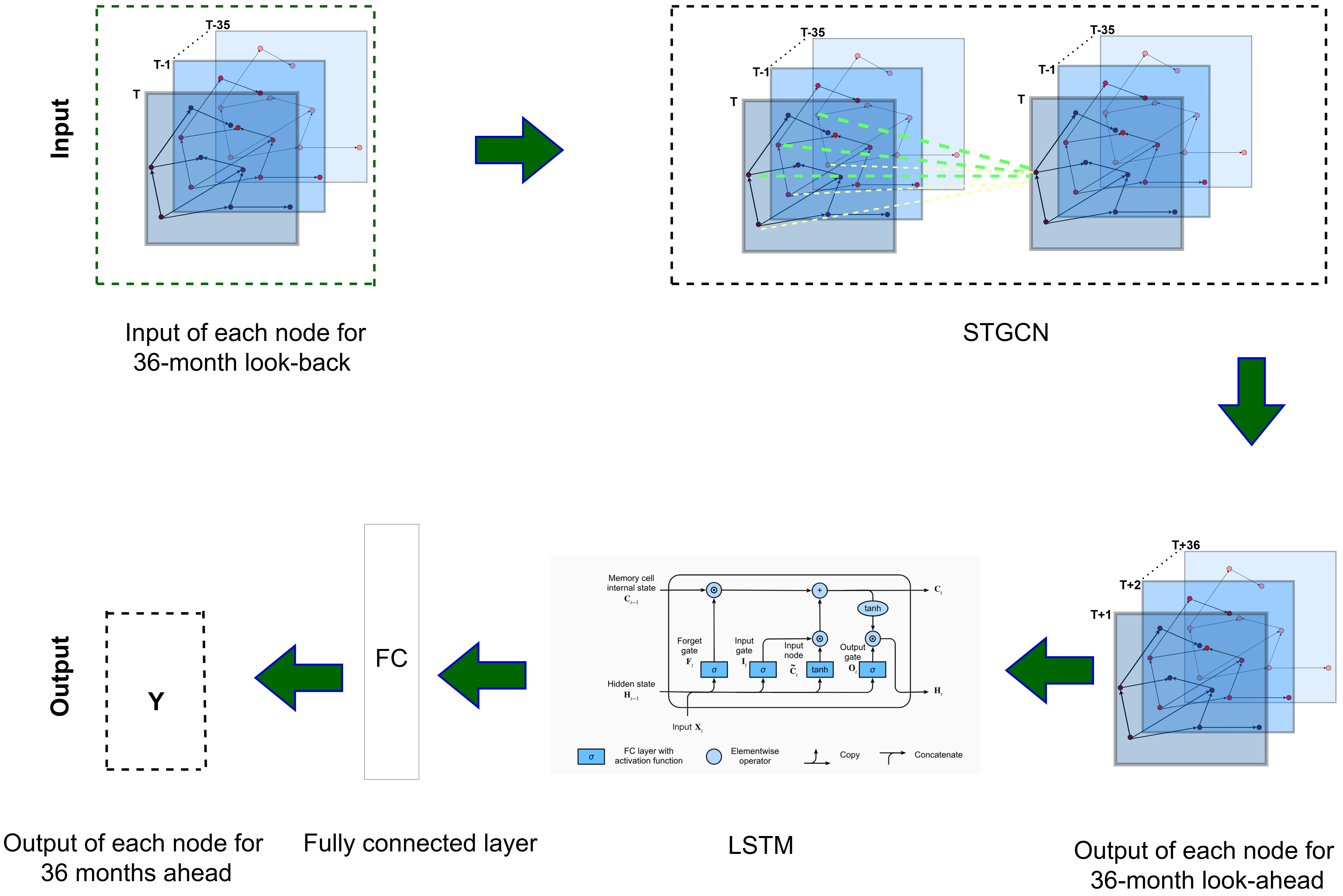
Figure 6 illustrates the proposed STGNN architecture, which integrates graph-based spatial modeling with recurrent network-based temporal modeling to generate multistep forecasts for streamflow at multiple monitoring stations. This architecture aligns with recent deep learning frameworks for hydrometeorological applications [71,72].

4.7. Overview of the STGNN Architecture

The core elements are as follows:

• Graph Convolutional Networks (GCNs): extracting spatial features through neighbor-based feature aggregation;
• LSTM: processing each station’s temporal sequence of GCN-generated embeddings to model temporal dependencies;
• Output Layer: generating multi-step predictions (e.g., 12-, 24-, or 60-month horizons) via a fully connected (FC) projection of the LSTM’s final hidden state.

4.7.1. Graph Construction

Node Set $\left(V\right)$

We define $V=\{v_1,v_2,\dots ,v_N\}$ as the set of N hydrological stations. Each $v_i$ corresponds to one USGS monitoring station, selected based on data availability and spatial coverage in the UCRB.

Adjacency Matrix (A)

The adjacency matrix $A\in {\{0,1\}}^{\left|V\right|\times \left|V\right|}$ encodes whether two stations share a direct hydrological connection within the river network. Each element $A_{ij}$ is defined as follows:

$$A_{ij}=\left\{\begin{array}{cc}1\hfill & \mathrm{if}\mathrm{station}{v}_i\mathrm{is}\mathrm{directly}\mathrm{connected}\mathrm{to}{v}_j,\hfill \\ 0\hfill & \mathrm{otherwise}.\hfill \end{array}\right.$$

(13)

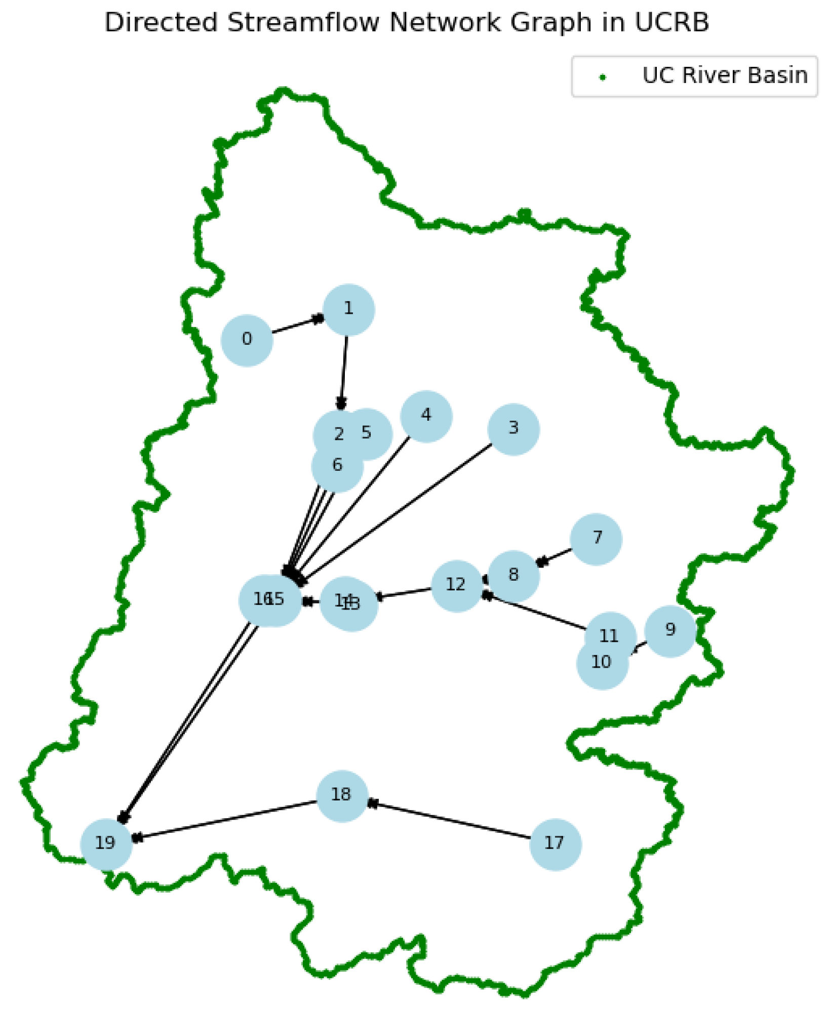
As illustrated in Figure 7, the connections within the graph network are based on the river basin’s inherent hydrographic structure, encompassing both the main channel and its tributary network. Monitoring stations located along the same river reach or nested within a shared sub-basin are considered neighbors, ensuring that the adjacency matrix A accurately represents the natural flow pathways within the basin. This approach allows the network to preserve the directional influences of upstream conditions on downstream flow, aligning with the inherent hydrological connectivity of the system [73,74,75].

4.7.2. Spatial Modeling Using GCN

The GCN layers embed each station’s features while integrating information from neighboring stations. The update rule for the GCN layers is expressed as follows:

$$H^{(l+1)}=\sigma \left(D^{-1/2}A{D}^{-1/2}{H}^{\left(l\right)}{W}^{\left(l\right)}\right)$$

(14)

where $H^{\left(l\right)}$ is the feature matrix at layer l, A is the adjacency matrix, D is the degree matrix, and $W^{\left(l\right)}$ is the trainable weight matrix. The output of the GCN layers captures spatial features that influence streamflow at each station.

By stacking multiple GCN layers, the model learns increasingly complex spatial representations. This enables each station’s embedding to reflect upstream and downstream flow influences, as stations within the same sub-basin share related hydrological patterns [76].

4.7.3. Temporal Modeling Using LSTM

Following the GCN layers, node embeddings are reshaped into sequences suitable for an LSTM module, which focuses on temporal dependencies. We adopt the standard LSTM formulation [61], in which the hidden and cell states ${\mathbf{H}}_t$ and ${\mathbf{C}}_t$ evolve over the input window (e.g., 12 months). The LSTM learns to capture both short-term dynamics (e.g., monthly variability) and longer-term trends (e.g., seasonal cycles). To achieve this, the GCN-produced embeddings for each node across all time steps are first flattened into an LSTM-compatible sequence. At each time step, the LSTM updates its hidden and cell states (${\mathbf{H}}_t$ and ${\mathbf{C}}_t$) based on both the current input and the previous states, thereby progressively refining the temporal representation. Once the final time step is reached (e.g., the T-th month), the last hidden state ${\mathbf{H}}_{\mathrm{end}}$ encapsulates the spatio-temporal information learned by the model, forming the foundation for subsequent predictions or analyses.

4.7.4. Output and Multi-Step Forecasting

A fully connected (FC) layer converts the final LSTM hidden state into a multi-step prediction:

$$\mathbf{Y}=\mathrm{FC}\left({\mathbf{H}}_{\mathrm{end}}\right)\in {\mathbb{R}}^{N\times p}$$

(15)

where p is the forecast horizon (e.g., 12, 24, or 60 months) and N is the number of stations. To mitigate overfitting, we optionally apply dropout [77], as also recommended in [71] for improving generalization in data-driven forecasting tasks.

4.8. Evaluation Metrics

In streamflow prediction, which is a regression task aimed at forecasting continuous values like streamflow, traditional metrics such as R² (coefficient of determination), RMSE (root mean square error), MAE (mean absolute error), and MAPE (mean absolute percentage error) are commonly employed. R² measures the proportion of variance in observed data that is predictable from the model, with values closer to 1 indicating a better fit. However, Legates and McCabe (1999) [78] noted the limitations of relying solely on R² and Pearson’s correlation coefficient (r), highlighting that these metrics can sometimes produce misleading results, especially when there are biases in the predictions.

More robust metrics like Nash–Sutcliffe efficiency (NSE) and Kling–Gupta efficiency (KGE) are often used in hydrological modeling to address these limitations. These metrics are better suited for evaluating streamflow models because they consider the correlation between predicted and observed values and errors in bias and variability [79,80].

$$\mathrm{RMSE}=\sqrt{{\displaystyle \frac{1}{n}}\sum _{i=1}^n{(f_i-r_i)}^2}$$

(16)

where $f_i$ is the predicted value and $r_i$ is the observed value. The RMSE quantifies the average difference between predicted and observed values.

$$R^2=1-{\displaystyle \frac{RSS}{TSS}}$$

(17)

where $RSS$ is the residual sum of squares, and $TSS$ is the total sum of squares. R² measures the proportion of variance explained by the model.

$$\mathrm{MAE}={\displaystyle \frac{1}{n}}\sum _{i=1}^n|f_i-r_i|$$

(18)

MAE represents the average absolute difference between the predicted and observed values.

$$\mathrm{MAPE}={\displaystyle \frac{1}{n}}\sum _{i=1}^n\left|{\displaystyle \frac{f_i-r_i}{r_i}}\right|\times 100$$

(19)

MAPE calculates the average absolute percentage difference between the predicted and observed values, providing a relative measure of prediction accuracy. However, the MAPE has limitations, such as its sensitivity to values near zero, which can lead to infinite or undefined percentage errors, and it may not be suitable for cases with large variability in the magnitude of the observations [81,82].

$$NSE=1-{\displaystyle \frac{{\sum }_{i=1}^n{(r_i-f_i)}^2}{{\sum }_{i=1}^n{(r_i-\overline{r})}^2}}$$

(20)

where $\overline{r}$ is the mean of the observed values. NSE assesses how well the model predicts relative to the mean of the observed data [79].

$$KGE=1-\sqrt{{(CC-1)}^2+{(\alpha -1)}^2+{(\beta -1)}^2}$$

(21)

where $CC$ is the correlation coefficient, $\alpha$ is the ratio of the variability in predicted and observed flows, and $\beta$ is the bias ratio between predicted and observed means. KGE refines the evaluation by considering correlation, bias, and flow variability [80].

Percent bias (PBIAS) measures the average tendency of the simulated values to be larger or smaller than the observed values. A positive PBIAS indicates model underestimation (underpredicting streamflow), while a negative PBIAS indicates model overestimation (overpredicting streamflow). A PBIAS value closer to zero is desirable, as it suggests minimal systematic bias in the model’s predictions [83].

$$\mathrm{PBIAS}=\left[{\displaystyle \frac{{\sum }_{i=1}^n(Y_{\mathrm{obs},i}-Y_{\mathrm{sim},i})\times 100}{{\sum }_{i=1}^n{Y}_{\mathrm{obs},i}}}\right]$$

(22)

where $Y_{\mathrm{obs},i}$ = observed streamflow value at time step i, $Y_{\mathrm{sim},i}$ = simulated (predicted) streamflow value at time step i, and n = total number of time steps.

Given the suitability of NSE and KGE for hydrological tasks, we have adopted them as key evaluation metrics in this research to assess the performance of our streamflow prediction models. By using these metrics, we provide a more reliable and robust evaluation than traditional metrics like R², RMSE, MAE, and MAPE. This approach offers a more comprehensive assessment of model performance, considering the intricacies of hydrological modeling.

5. Results

In this section, we present the detailed experimental results of our analysis, which are divided into two subsections. (1) Comparison of Five Machine Learning Models evaluates STGNN, GRU, LSTM, SARIMA, and RFR across multiple performance metrics. (2) Sequence Analysis for STGNN examines how varying the input (look-back) and output (look-ahead) lengths influences the predictive accuracy of the proposed STGNN model.

In our analysis, we tested various look-back (input) and look-ahead (output) configurations to determine the optimal setup for streamflow forecasting. Using 36 months of historical data to predict 36 months ahead provided the best balance for model training and testing. Sequential analysis revealed that while performance improves with longer input and output windows, it declines beyond a certain threshold, leading to higher errors. Five evaluation metrics (described in Section 4.8) were used to quantify accuracy, and prediction-versus-observation plots were generated to provide a clear perspective on model performance.

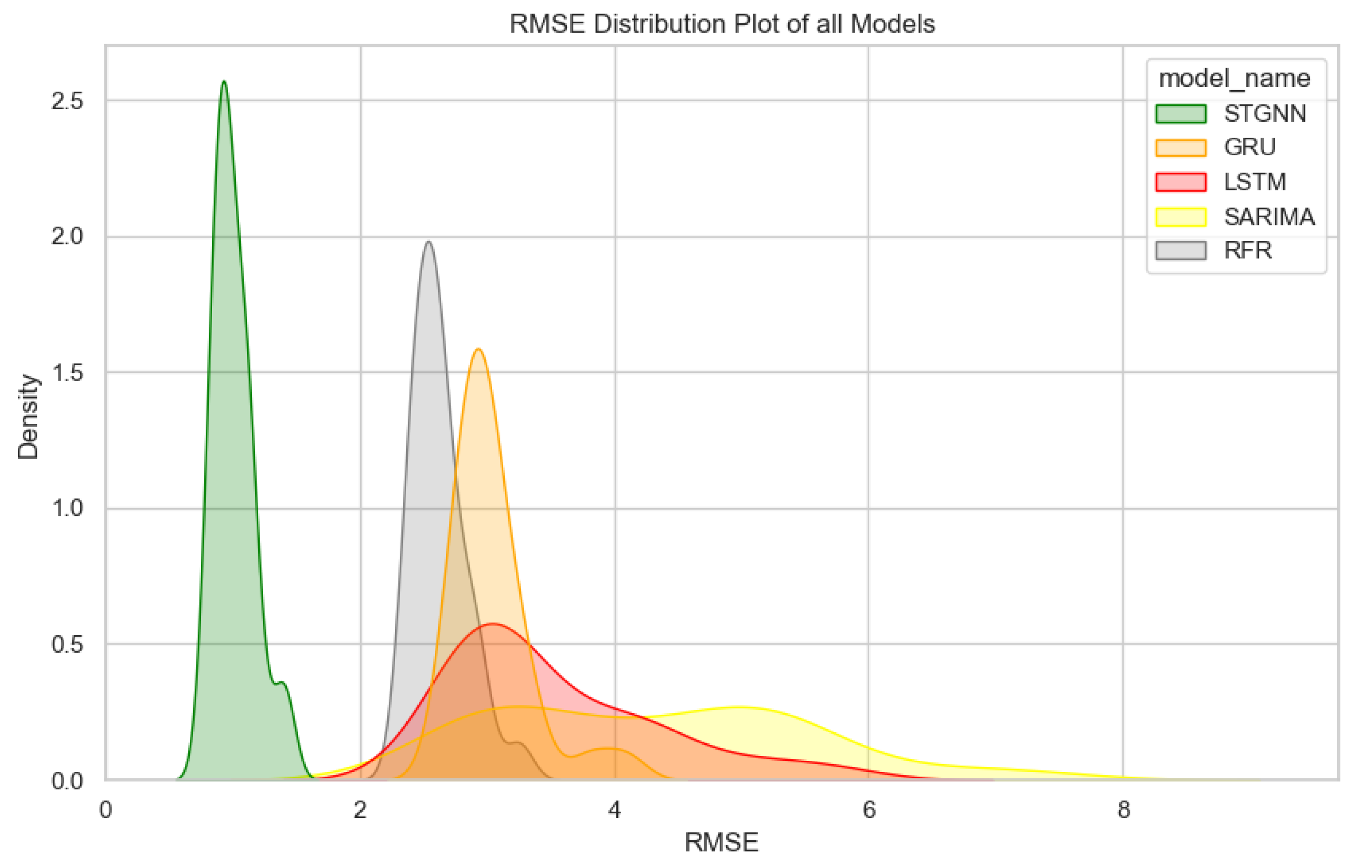
The comparison of the five models starts with an analysis of the RMSE distribution shown in Figure 8.

The STGNN model demonstrates the lowest median RMSE value of approximately 1.0 mm/month, with a narrow spread, indicating minimal variability in prediction errors. In contrast, SARIMA and LSTM exhibit significantly wider distributions, indicating high variability and uncertainty in their predictions. This inconsistency suggests that these models struggle with generalization across the dataset, making them less reliable for streamflow forecasting. The GRU model performs moderately well, with a narrower spread compared to SARIMA and LSTM, but its median RMSE value of approximately 2.5 mm/month remains higher than desired, highlighting its limitations in achieving low error rates. RFR, while more consistent than GRU in terms of error spread, achieves a median RMSE value of around 2.3 mm/month, which, although better than that of GRU, is still higher than that of STGNN. Moreover, the peak of RFR’s distribution is less pronounced than that of STGNN, indicating that its predictions are not as concentrated within a narrow error range.

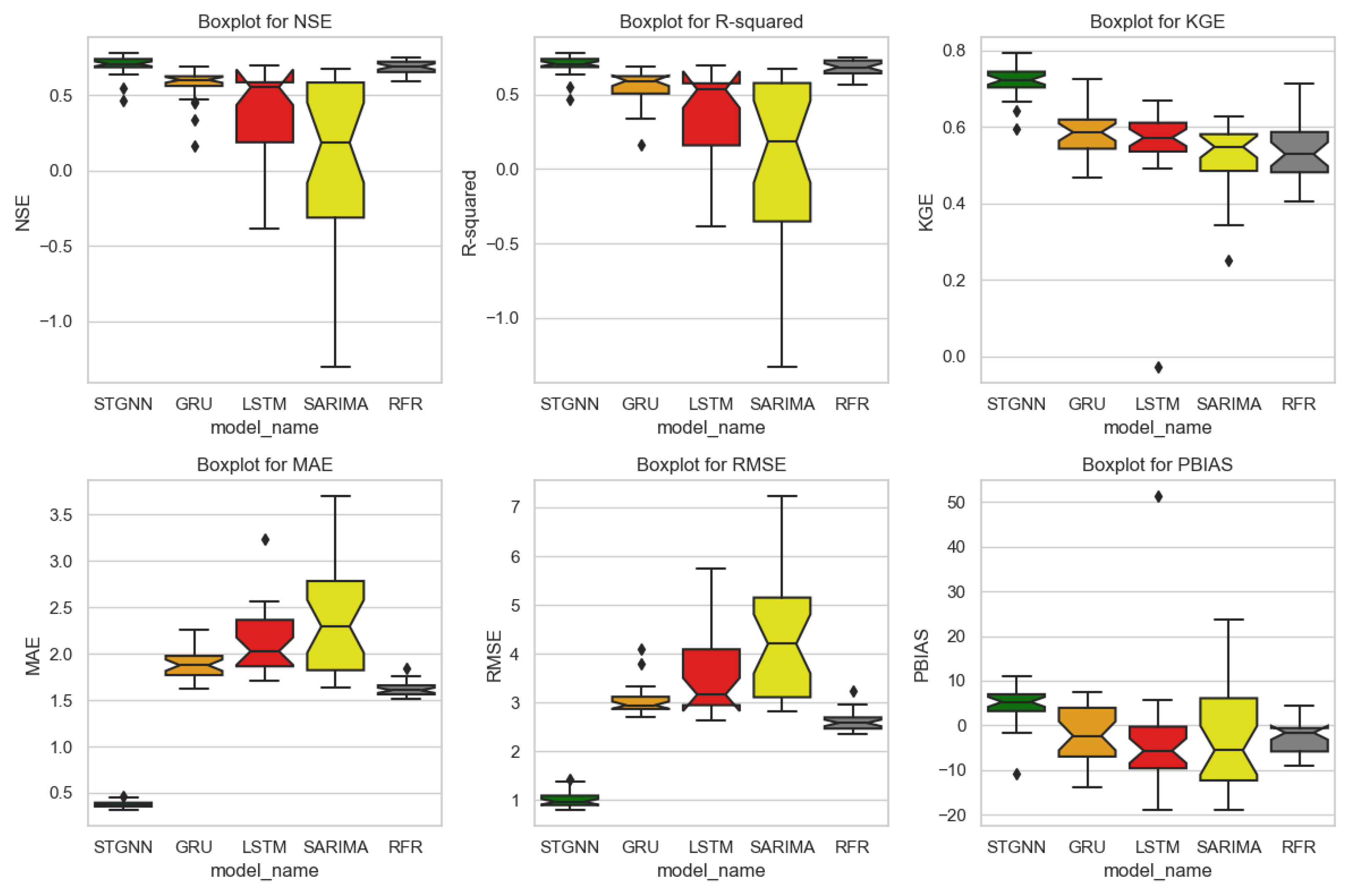
Figure 9 presents the box plots for five key performance metrics, NSE, R², KGE, MAE, and RMSE, evaluated across the five machine learning models. The STGNN model showcases the highest median values for NSE (0.71), R² (0.71), and KGE (0.72), with the narrowest interquartile ranges across these metrics. This indicates that STGNN produces highly consistent and reliable predictions. Moreover, STGNN achieves the lowest median RMSE (0.97 mm/month) and MAE (0.37 mm/month), highlighting its ability to generate highly accurate forecasts with minimal error. The tight clustering of RMSE and MAE values confirms the robustness of STGNN, making it the most reliable model for streamflow forecasting among the tested approaches.

In contrast, SARIMA shows the weakest performance, with the lowest median NSE (0.18) and R² (0.18) values, and the widest spread for RMSE (4.20 mm/month) and MAE (2.29 mm/month). These results highlight SARIMA’s inability to model the non-linear dynamics of streamflow. Similarly, LSTM demonstrates moderate performance but struggles with variability, achieving a median NSE of 0.55 and R² of 0.53, with RMSE and MAE medians of 3.17 mm/month and 2.03 mm/month. Its broader interquartile ranges suggest difficulty maintaining prediction stability.

The GRU model performs better than LSTM, with a median NSE of 0.60 and R² of 0.59, and RMSE and MAE medians of 2.95 mm/month and 1.88 mm/month. While GRU shows improved consistency over SARIMA and LSTM, its error levels remain higher than those of STGNN. RFR achieves competitive results, with median NSE and R² values of 0.69 and 0.68, and a lower RMSE (2.58 mm/month) and MAE (1.61 mm/month) than GRU. However, its broader error spread compared to STGNN indicates less stability.

The PBIAS box plot in Figure 9 highlights the bias distribution across models. SARIMA exhibited the most inconsistent PBIAS, reflecting its difficulty in modeling non-linear streamflow dynamics. GRU and LSTM showed relatively balanced PBIAS distributions, though with wider variability, suggesting occasional fluctuations in their predictive bias. RFR maintained a near-zero median PBIAS, indicating minimal systematic bias but greater variance across different time periods. Initially, STGNN showed a positive PBIAS, suggesting a slight underestimation of streamflow values. To address STGNN’s systematic bias, we applied linear bias correction (LBC), a widely used post-processing technique for model calibration [84]. The research supports simple scaling as an effective method to reduce systematic errors in hydrological and machine learning models [85,86]. By implementing this correction, we successfully eliminated systematic bias in STGNN predictions while preserving its temporal-spatial learning capabilities.

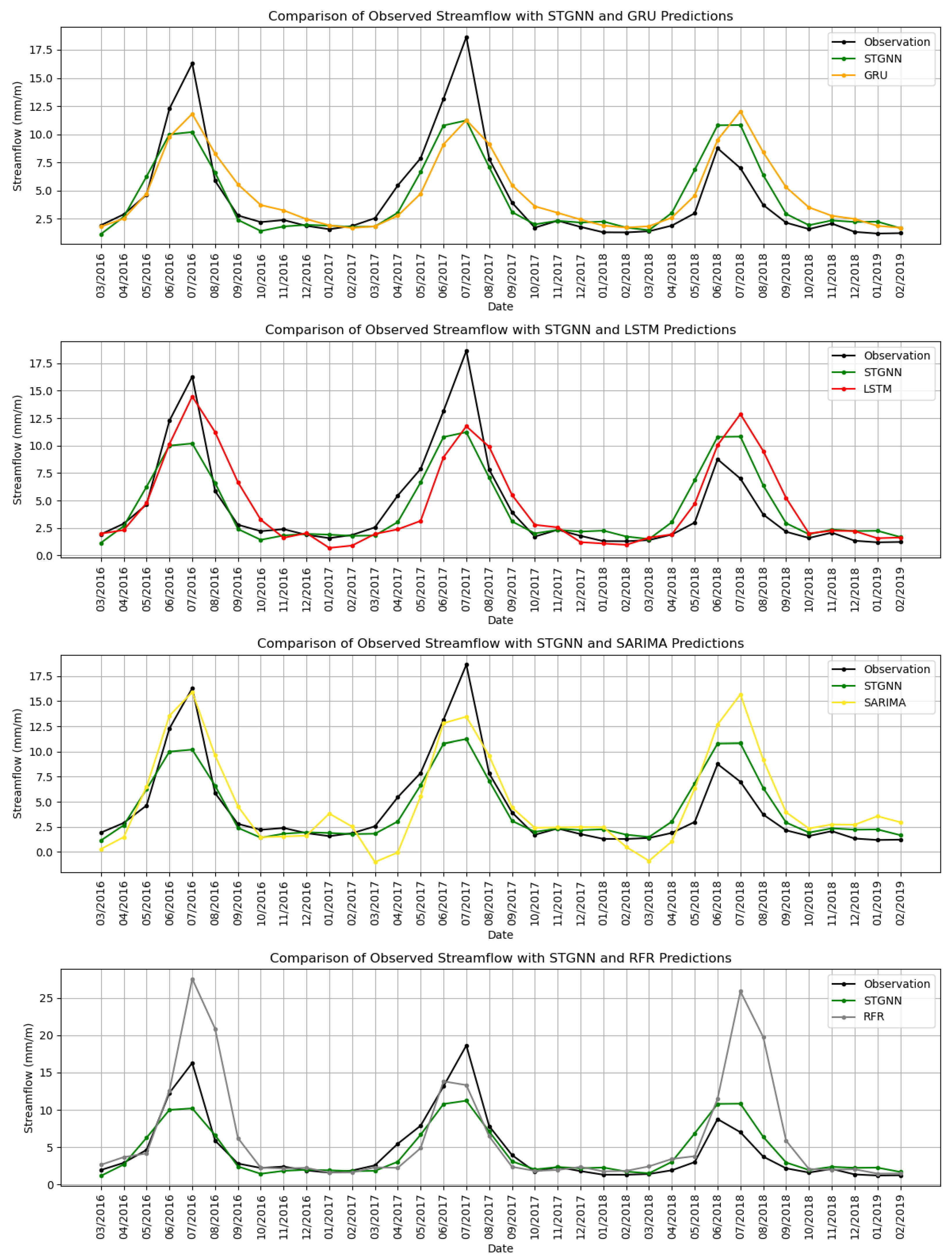
Figure 10 shows a comparison of observed streamflow against the predictions made by the models over the testing period from March 2016 to February 2019. The predictions represent a 36-month forecast, highlighting the ability of each model to capture both seasonal variations and peak flow magnitudes.

The STGNN model shows strong alignment with observed streamflow, effectively capturing seasonal peaks and baseflow periods with minimal deviation. Its predictions closely follow the observed streamflow during high-flow periods, such as mid-2017 and mid-2018, and maintain consistency across low-flow intervals. The GRU model, as shown in the top panel, performs well in tracking the general trend of streamflow but shows noticeable deviations during peak flow periods. For instance, it overestimates the peak flow in mid-2017 and underestimates flow during recessional periods, indicating some limitations in capturing rapid changes. The LSTM model, shown in the second panel, struggles more significantly, overestimating peak flows during high-flow periods and exhibiting greater variability during low-flow intervals.

The SARIMA model, shown in the third panel, fails to accurately capture peak flows and introduces higher variability during low-flow periods. Its underestimation of flow magnitude during critical periods, such as mid-2017 and mid-2018, demonstrates its limitations in handling the non-linear and dynamic nature of streamflow. RFR, illustrated in the bottom panel, shows improved performance during baseflow conditions but tends to overestimate peak flows, such as during mid-2018. This suggests that while RFR performs better than SARIMA in certain conditions, it still lacks the accuracy and stability required for precise streamflow forecasting.

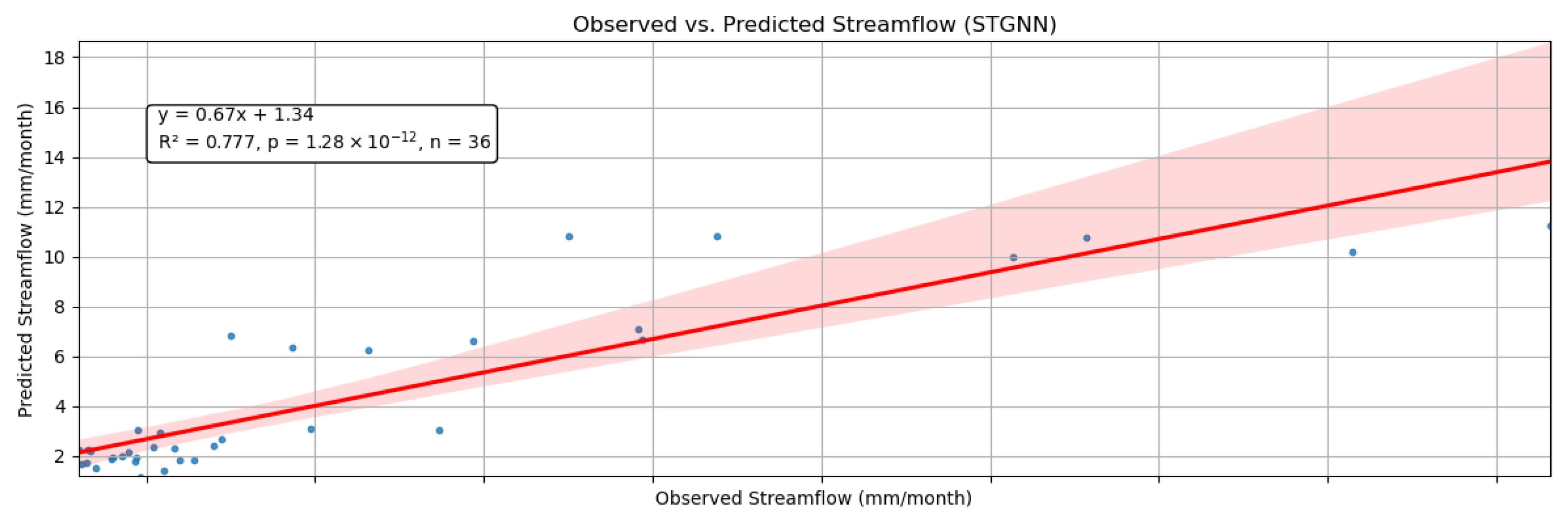
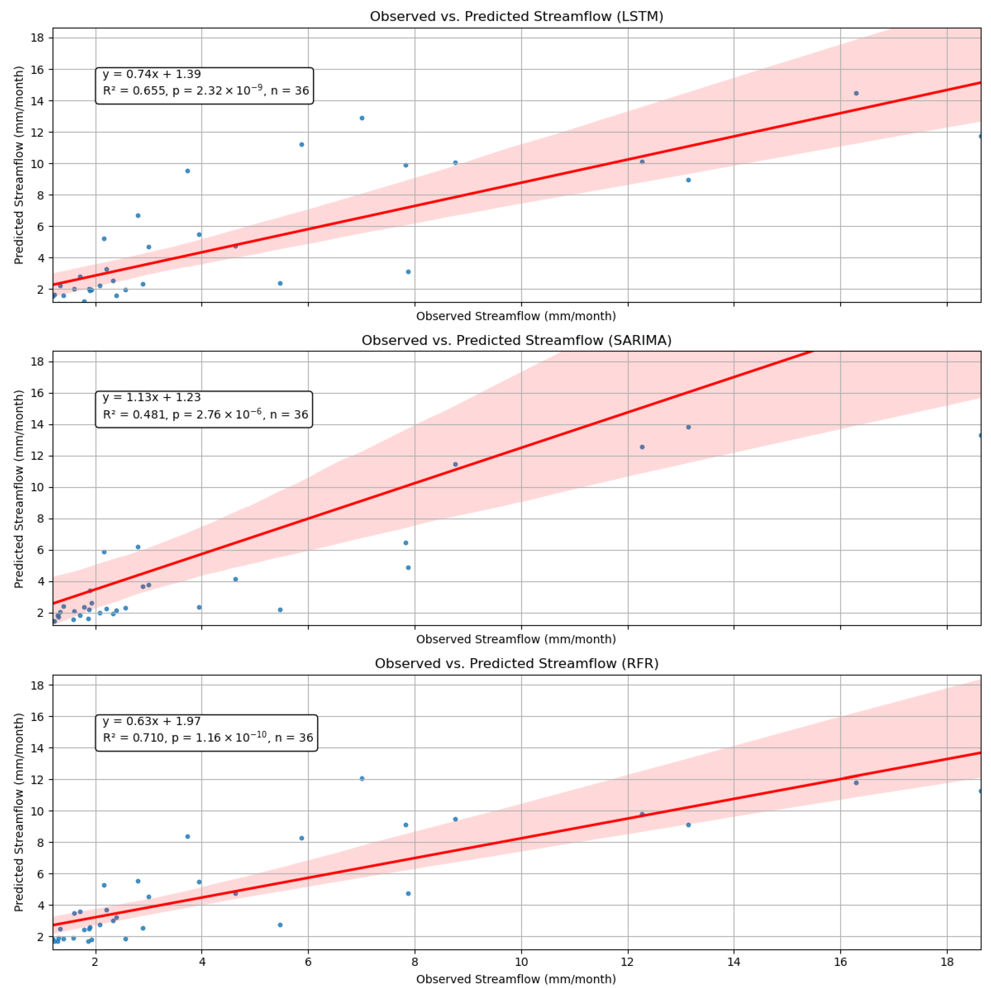
To further assess model performance and highlight approximation errors, we plotted observed–predicted correlation graphs with regression lines in Figure 11. These plots provide a clearer visualization of prediction trends, showcasing the strengths and limitations of each model. The STGNN model demonstrates strong agreement with observed values, effectively capturing overall trends while slightly underestimating extreme peak flows. The LSTM model follows the general pattern but exhibits greater variability, often overestimating high-flow events. The SARIMA model shows significant underestimation of peak flows, reflecting its limitations in handling non-linear streamflow variations. The RFR model performs well in baseflow conditions but tends to overpredict high streamflow values, leading to increased dispersion at larger magnitudes. Each plot includes a linear regression equation quantifying the relationship between observed and predicted streamflow. R² values range from 0.481 (SARIMA) to 0.777 (STGNN), reflecting varying predictive accuracy. Low p-values confirm statistical significance, with a consistent sample size n = 36 across models. STGNN and RFR slightly underestimate streamflow, while SARIMA’s slope $>1$ suggests overestimation at lower magnitudes. The regression lines and confidence intervals highlight model deviations and alignment with observed data.

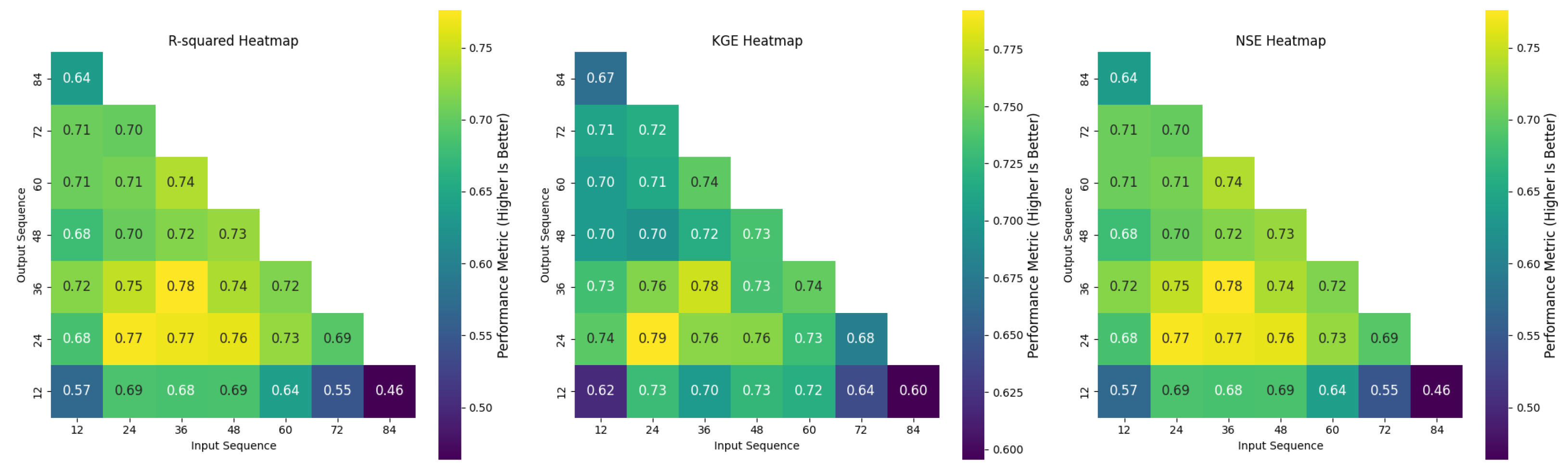
6. Sequence Analysis for STGNN Model

The sequence analysis evaluated the impact of varying input (look-back) and output (look-ahead) sequence lengths on the STGNN model’s performance. A total of 28 combinations were tested, including (12, 12), (12, 24), (12, 36), (12, 48), (12, 60), (12, 72), (12, 84), (24, 12), (24, 24), (24, 36), (24, 48), (24, 60), (24, 72), (36, 12), (36, 24), (36, 36), (36, 48), (36, 60), (48, 12), (48, 24), (48, 36), (48, 48), (60, 12), (60, 24), (60, 36), (72, 12), (72, 24), and (84, 12). This comprehensive analysis provides insights into the trade-offs between shorter and longer input–output sequences, helping identify the optimal configuration for streamflow forecasting.

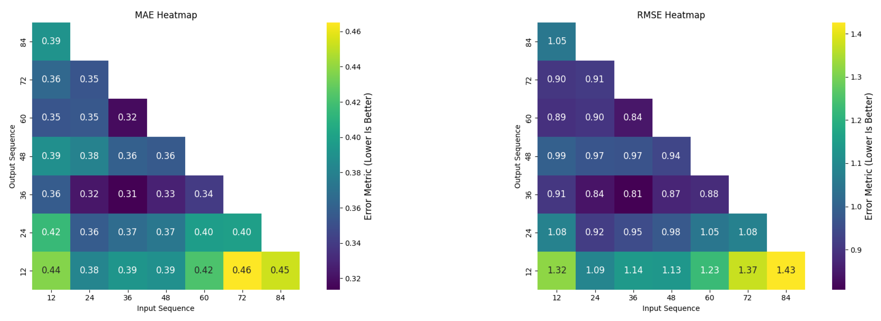
Figure 12 shows heatmaps for R², NSE, and KGE, while Figure 13 displays the MAE and RMSE across sequence combinations. Configurations like (24, 24) and (36, 36) consistently performed well. The (36, 36) configuration achieved slightly better results (R²: 0.78, NSE: 0.78, KGE: 0.79) than (24, 24) (R²: 0.77, NSE: 0.77, KGE: 0.74), indicating its superior ability to capture input–output relationships. The error metrics displayed in Figure 13 demonstrated a similar trend. The (36, 36) configuration achieved the lowest RMSE (0.81 mm/month) and MAE (0.32 mm/month), compared to the (24, 24) configuration, which had an RMSE of 0.92 mm/month and MAE of 0.36 mm/month. These results highlight that while both configurations perform well in terms of correlation, the (36, 36) setup minimizes prediction errors more effectively, making it the optimal choice for this dataset.

The MAE heatmap in Figure 13 highlights the importance of moderate input–output combinations. Shorter sequences, like (12, 12), had higher MAE values (0.44 mm/month), indicating insufficient historical data, while longer sequences, such as (48, 48), showed diminishing returns, with the MAE increasing to 0.34 mm/month.

The RMSE heatmap in Figure 13 supports this, as configurations beyond (48, 48) exhibited higher errors. The (36, 36) configuration, with the lowest MAE and RMSE, demonstrates the effectiveness of balancing sequence length for optimal predictions.

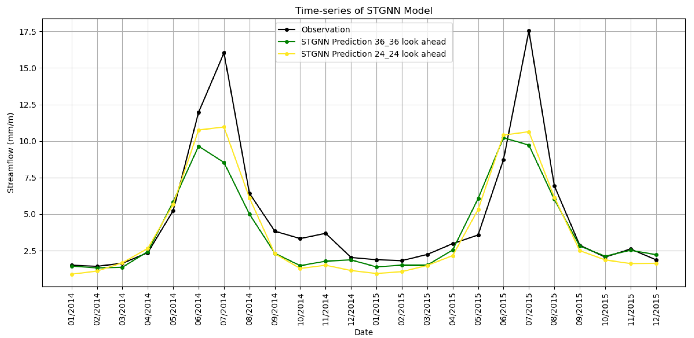
The comparison of STGNN predictions for the (24, 24) and (36, 36) configurations, shown in Figure 14, further supported these findings. The (36, 36) configuration more accurately captured both the magnitude and timing of seasonal peaks compared to (24, 24). During the high-flow period in mid-2015, the (36, 36) predictions aligned more closely with observed streamflow, while the (24, 24) configuration underestimated the peaks. These differences emphasized the advantage of the (36, 36) setup in leveraging additional temporal information for more accurate long-term forecasts. Beyond the (36, 36) configuration, performance began to decline as sequence lengths increased. The (48, 48) configuration showed a slight drop in R² to 0.73 and an increase in RMSE to 0.94 mm/month, highlighting the diminishing returns of excessively long input–output sequences. Longer sequences introduced unnecessary complexity and noise, reducing the model’s ability to generalize effectively.

Figure 15 illustrates the impact of varying input (look-back) lengths on STGNN predictions. Shorter look-back windows, such as 12 or 24 months, led to underestimations during high-flow periods and greater variability during baseflow periods. In contrast, longer look-back windows, such as 36 and 48 months, improved the model’s ability to capture both high and low flows. However, increasing the look-back length to 60 months introduced inconsistencies, such as overestimations during certain periods. This suggested that excessively long input sequences reduced predictive accuracy since they may introduce noise or irrelevant historical data, which complicate the model’s ability to generalize effectively. The 36-month look-back emerged as the most effective configuration, striking a balance between capturing sufficient historical context and avoiding unnecessary complexity.

7. Discussion

The proposed STGNN model demonstrated a significant advancement in streamflow prediction accuracy compared to traditional methods, including SARIMA, RFR, LSTM, and GRU. By integrating spatial connectivity through GCNs and capturing temporal dynamics with LSTM layers, the STGNN consistently outperformed these models across multiple metrics, including NSE, R², RMSE, and KGE.

The integration of spatial and temporal features was a critical factor in the enhanced predictive performance of the STGNN. Studies have highlighted the importance of spatial connectivity in hydrological modeling, demonstrating how incorporating spatial relationships improves prediction accuracy [18,31]. Similarly, spatially aware machine learning models significantly enhance streamflow predictions in ungauged basins [34]. These insights align with our approach, where an adjacency matrix representing hydrological connectivity was used to capture interdependencies between river nodes. For instance, at critical locations such as Lees Ferry, the STGNN achieved an R² value of 0.78, outperforming GRU and LSTM models, which achieved R² values of 0.60 and 0.55, respectively. This result corroborates findings on the effectiveness of spatio-temporal graph-based methods in capturing streamflow dynamics under varying climatic conditions [36].

Spatio-temporal machine learning models are increasingly recognized as valuable tools in hydrological applications. Attention-based spatio-temporal models have been used for drought forecasting, showcasing their capability to capture complex interdependencies across space and time [87]. Similarly, hybrid spatio-temporal neural networks for rainfall-runoff modeling have highlighted the importance of integrating spatial interactions with temporal sequences [88]. These studies reinforce the value of spatio-temporal frameworks like STGNN in effectively combining spatial and temporal features, leading to superior predictive performance compared to traditional methods.

Among traditional ML models, RFR demonstrated notable performance in streamflow prediction, particularly in multivariate setups. Research has emphasized the advantages of multivariate models [60,89] but our research, focusing exclusively on streamflow data, found that RFR still outperformed SARIMA, LSTM, and GRU. The robustness of RFR in capturing non-linear relationships and avoiding overfitting highlights its adaptability across diverse hydrological conditions [60,90]. Furthermore, the limitations of SARIMA in addressing non-linear dynamics, such as its lower NSE and higher RMSE values compared to STGNN, were evident in our findings [91]. These results underscore the importance of advanced data-driven models like RFR and STGNN in addressing the complexities of streamflow prediction, particularly in heterogeneous basins such as the UCRB.

Traditional models like SARIMA have often been noted for their reliability in long-term forecasts, particularly under specific conditions like droughts [91]. However, their performance is often hindered by limitations in handling non-linearities and spatial variations in streamflow data. While SARIMA requires significant hyperparameter tuning, it often falls short when compared to data-driven models like STGNN. Despite these shortcomings, SARIMA remains a viable option for long-term streamflow predictions, especially when larger datasets are available [91].

Despite its strong performance, the study has some limitations. The model struggled to fully capture extreme peak flows, likely due to their infrequent occurrence in the training data. Additionally, while STGNNs excel in modeling spatial relationships, their computational demands increase with larger networks, which could pose scalability challenges for broader applications. The reliance on historical streamflow data also underscores the need for integrating additional hydrometeorological variables to enhance predictive robustness.

Our sequence analysis further demonstrated the importance of optimizing input–output configurations in spatio-temporal models. Previous studies explored the trade-offs associated with varying sequence lengths [39,92], and consistent with these findings, our research identified the (36, 36) configuration as optimal. This setup achieved NSE, R², and KGE values of 0.78, 0.78, and 0.79, respectively, balancing the historical context and forecast horizon. It outperformed shorter sequences like (12, 12) and longer ones like (48, 48). These results align with observations that emphasize the need for careful sequence optimization in spatio-temporal models for hydrological forecasting [36].

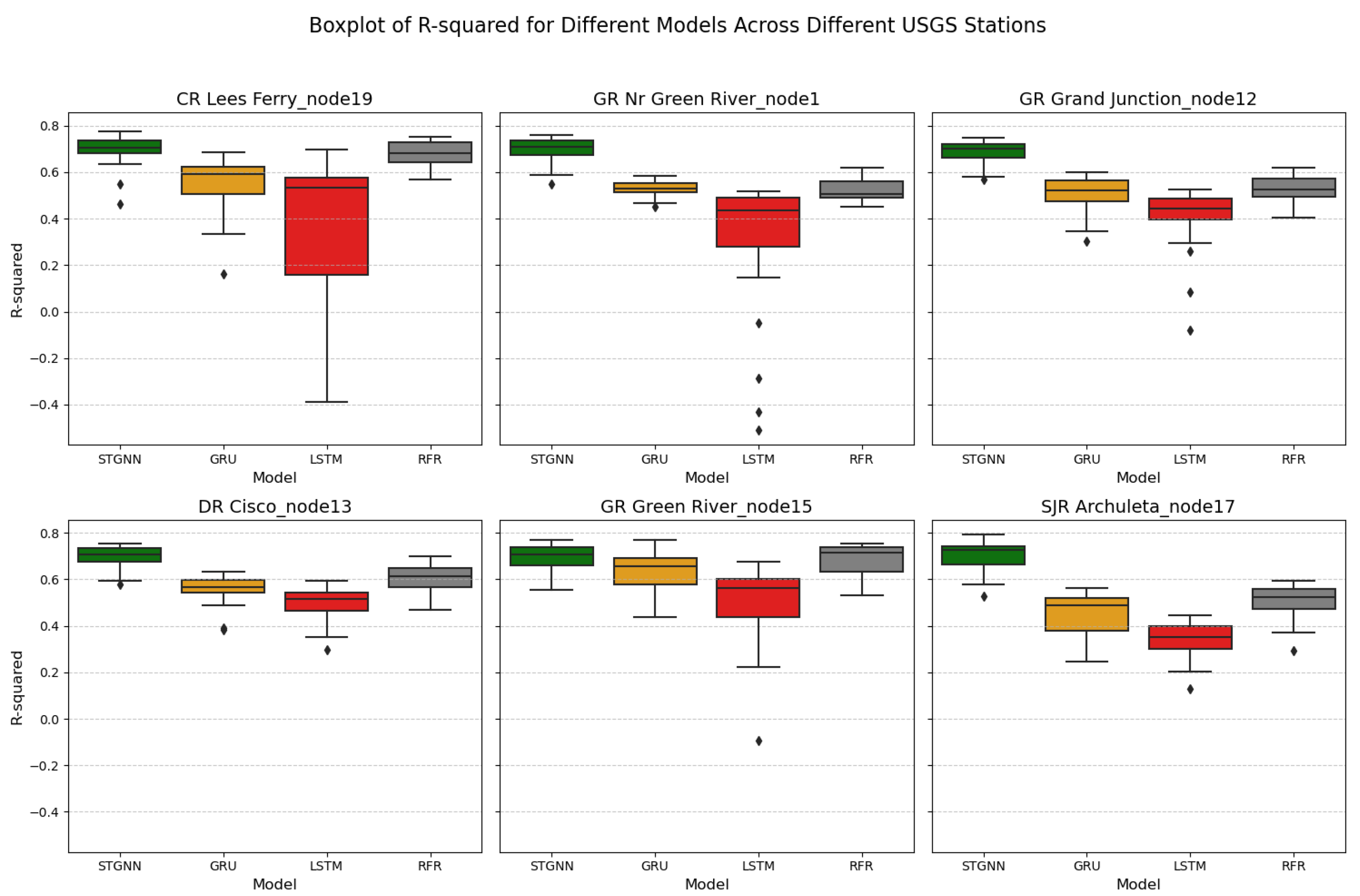
The boxplots in Figure 16 illustrate the R² performance of STGNN, GRU, LSTM, and RFR across six strategically selected USGS stations within the Upper Colorado River Basin. These stations—GR Nr Green River (Node 1), Grand Junction (Node 12), Cisco (Node 13), Green River (Node 15), Archuleta (Node 17), and Lees Ferry (Node 19)—were chosen to represent diverse sub-basins and critical flow convergence points, ensuring the evaluation of model performance under varying hydrological and geographical conditions.

Each station highlights key aspects of the basin’s flow dynamics. For instance, Node 1 (GR Nr Green River) integrates upstream tributary inflows, while Node 12 (Grand Junction) captures the confluence of the Gunnison River with the Upper Colorado. Node 17 (Archuleta) represents the San Juan sub-basin before its downstream merger, and Node 19 (Lees Ferry) serves as the primary evaluation point for the basin. Mid-basin nodes like Node 13 (Cisco) and Node 15 (Green River) assess performance in regions with moderate streamflow. Across these stations, STGNN consistently achieves the highest median R² values, showcasing robust generalizability. For example, at Lees Ferry (Node 19), STGNN achieves a median R² of approximately 0.78, demonstrating strong predictive accuracy. Similarly, at Green River (Node 1), Grand Junction (Node 12), and Archuleta (Node 17), STGNN outperforms GRU, LSTM, and RFR with higher median R² values and reduced variability. While STGNN achieves a median R² of approximately 0.75 at Green River (Node 15), its performance is comparable to that of RFR, but with narrower interquartile ranges, indicating greater consistency.

These findings underscore the strength of STGNN in capturing flow dynamics across diverse hydrological conditions, including those with moderate or low streamflow. While both STGNN and RFR perform well at certain nodes, such as Green River (Node 15), STGNN consistently shows higher median R² values and narrower interquartile ranges across most stations, indicating greater robustness and reduced error variability. The model’s consistent performance across geographically varied stations, such as Lees Ferry (Node 19) and Archuleta (Node 17), highlights its adaptability and generalizability beyond specific training locations. This robust performance positions STGNN as a reliable tool for streamflow forecasting in heterogeneous basins, a critical requirement for effective water resource management in regions with varying flow regimes.

Building on the strengths of this study, future research could explore incorporating precipitation, snowfall, soil moisture, and evapotranspiration data to further enhance model accuracy. Furthermore, refining the adjacency matrix construction by using correlation-weighted edges could improve the representation of hydrological connectivity. Implementing scalable graph partitioning and adaptive graph sampling techniques may enhance computational efficiency, enabling STGNNs to model larger hydrological networks. To further improve generalization, ensemble learning methods and transfer learning approaches could mitigate overfitting, particularly in data-scarce regions. Optimizing STGNN architectures for real-time operational use, particularly in reservoir management and flood forecasting, is another promising direction. These advancements will expand the applicability of STGNNs, making them even more versatile and effective in addressing the complexities of hydrological forecasting.

8. Conclusions

This study utilized a spatio-temporal graph neural network (STGNN) model for streamflow prediction in the Upper Colorado River Basin, leveraging graph convolutional networks (GCNs) for spatial dependencies and long short-term memory (LSTM) networks for temporal dynamics. Through rigorous evaluation against traditional methods such as seasonal autoregressive integrated moving average (SARIMA), random forest regression (RFR), LSTM, and gated recurrent units (GRU). The STGNN showed superior performance, achieving an R² of 0.78 and a KGE of 0.79 at critical nodes, like Lees Ferry. It also achieved the lowest median RMSE of 0.81 mm/month and a median MAE of 0.32 mm/month, reflecting its ability to generate highly accurate predictions with minimal errors. The configuration (36, 36), which uses 36 months of historical data to forecast 36 months, emerged as the optimal setup, balancing predictive accuracy, model complexity, and error minimization.

Potential future research could focus on integrating meteorological data, such as snow precipitation and temperature, to enhance model accuracy. Exploring advanced graph representation techniques with weighted edges could improve the understanding of hydrological relationships. Furthermore, adapting STGNN models for real-time applications, including reservoir management and flood forecasting, would be a promising direction for operational hydrology.