Plantwide Control for the Separation of THF-H₂O in an Azeotropic Distillation Process

Abstract

This paper presents a plantwide control strategy for optimizing a pressure-swing azeotropic distillation process used in tetrahydrofuran dehydration. Leveraging Skogestad’s methodology, this strategy focused on two distillation columns: a low-pressure column for water recovery at 20 psia and a high-pressure column that achieved 0.99 molar fraction purity of tetrahydrofuran at 115 psia. This study identified critical control variables through plant analysis by implementing PI controllers in the regulatory control layer to stabilize flows and pressures. In the supervisory control layer, a PI controller combined with MIMO MPC effectively enhanced the product purity and reduced the energy consumption by 36%. Stable inlet and outlet flow conditions (100 lbmol/hr inlet, 29.59 lbmol/hr outlet) were maintained without compromising the equipment integrity. The operational ranges for the process included variations in the tetrahydrofuran mole fraction from 0.25 to 0.35 at the inlet, which demonstrated a robust performance across perturbations. These achievements signify significant advancements in process efficiency and sustainability, offering substantial reductions in energy usage while ensuring consistent high purity levels in tetrahydrofuran production. The developed control structure sets a new standard for efficient azeotropic distillation processes, with implications for enhancing operational performance across industrial applications.

1. Introduction

In many industrial processes, strategically optimizing operations to enhance raw materials and energy use is crucial. The key is to achieve these objectives without significant investment while improving the operation and control of each piece of equipment in a plant. Instead of designing control systems individually for each process unit, a more strategic approach is to implement plantwide control [1,2,3,4,5].

In some chemical plants, the complexity is such that we find hundreds of variables that must be measured and controlled. Over the years, various methods have been developed to optimize the energy and raw materials in these processes. One of the pioneering works was that of Buckley [6], who proposed complete plant control techniques that were gradually perfected. In addition to the different techniques, architectures also emerged to design the control of an entire plant, as explained by Ochoa et al. [7], who classified these architectures into four main groups and characterized them by the system’s complexity.

Luyben [8] described a hierarchical plantwide methodology divided into nine levels, each combining heuristic rules applied in several process cases. Larsson and Skogestad [9] studied different methodologies of plantwide control and classified them in terms of a focus on simulation and a focus on mathematical and optimization models.

Several real-world examples demonstrated the application of plantwide control methodologies. For instance, Araújo and Skogestad [10] implemented the complete plant control methodology in the ammonium synthesis process. Gera et al. [11] developed a selection procedure for the primary controlled variables of the Skogestad methodology in the Cumene manufacturing process. Panahi and Skogestad [12] used the methodology to optimize the operation of an economical CO₂ capture process. Jagtap et al. [13] conducted a steady-state analysis to study three realistic examples of processes. These studies followed a systematic approach, including the determination of unrestricted degrees of freedom, consistent mass balances, the definition of primary controlled variables, and the location of the manipulator’s performance. Minasidis et al. [14] presented a complete plant control design based on the methodology of Skogestad [15] and evaluated the economic performance of a chemical process plant consisting of a reactor, a separator, and a recycling flow with purge. The primary variables were determined from local methods, and the control structures performed well under large perturbations in the system. Gera et al. [11] presented the results of a control structure designed using the Skogestad methodology in the Cumene production process to maximize the production of the process. In addition, all degrees of freedom were optimized in a steady state to obtain more significant benefits.

One of the most popular plantwide control structures was presented by Skogestad [16]; the design consists of a top-down analysis and a bottom-up design. The top-down analysis begins with defining the operational objectives, identifying the manipulated variables and degrees of freedom (DOF), then optimizing, and finally selecting the primary variables for control ($C{V}_1$). In contrast, the bottom-up design starts with the stabilizing the control layer (regulatory layer) and the supervisory controller ($C{V}_2$) and ends with providing integration with the optimization layer.

During the top-down step, an important decision involves selecting economic controlled variables ($C{V}_1$). In the bottom-up step, a key decision involves selecting stabilizing controlled variables ($C{V}_2$). The $C{V}_1$ variables often act as active constraints and are sometimes transferred to the fast regulatory layer as part of $C{V}_2$.

Some examples that implemented this type of control are the following: complete plant control for the oil production process [17]; biodiesel production to maintain product quality [18]; an economic plantwide control for the cumene process [19]; the capture of CO₂ by absorption and stripping using a monoethanolamine solution [20]; and we can observe that implementation of this type of control is used in large chemical processes such as the HDA process [10], or in this case, the separation of a mixture.

Separating azeotropic THF–water mixtures is crucial for various industrial processes, like polymer and pharmaceutical production. Effective separation is essential for maintaining purity, reducing costs, and minimizing the environmental impact. Improved separation also supports recycling, cost effectiveness, and advances in research and development. This process has been widely studied: In [21], a comparison between extractive and pressure-swing distillation was analyzed to separate the THF–water mixture. Two flowsheets to separate this mixture were compared in [22]. In [23], a criterion to select an entrainer in extractive distillation to separate the THF–water was studied. Bartokova et al. [24] studied how to separate THF–water using stearic acid. Another method to separate the mixture involves using a batch extractive distillation, as mentioned in [25]. They used the HYSYS process simulator to verify the results, and the compound 1,2 propanediol was selected as the separation agent for the distillate mixture. In Chapman et al. [26], they used pervaporation distillation to separate this mixture with a combined membrane. A study of azeotropic distillation with pressure changes was carried out, integrating heat externally in one of the columns [27]. They analyzed the costs in a plant without and with this provision of heat energy. In Zhang et al. [28], they selected a solvent to separate this mixture through extractive distillation.

Also, the THF–water separation processes have several variables that must be controlled, such as pressure, heat, and/or reflux ratios, as presented in [29]. They presented dynamic control of the reflux ratio and reboiler heat duty. Additionally, they added a thermal integration process. In [30], a heat integration and dynamic control strategy of reactive pressure-swing distillation to separate the mixture was applied. In [31], a dynamic controllability study was applied to extractive and pressure-swing distillation; they controlled the feed flow, pressures, reflux drum levels, and temperatures in trays using PI controllers.

Azeotropic processes involve multiple interacting loops, where changes in one part of the process affect others due to the fixed composition behavior at the azeotropic point. Skogestad’s method considers these interactions explicitly, aiming to optimize the overall process performance by minimizing the disturbances and maximizing the control effectiveness across the entire plant. By optimizing the overall plant operation, Skogestad’s method can lead to reduced energy consumption. Also, this approach ensures that the control system operates closer to optimal conditions, minimizing waste and improving the overall process efficiency. This efficiency can translate into higher yields and a better quality of the final product. The field of opportunity to use this methodology is in mixtures of bioethanol and water to reach the biofuel standards.

The contributions to this research using Skogestad’s methodology in the process of pressure-swing azeotropic distillation for the separation of THF-H2O are the following: optimization of the operation of the process that consumes less energy without altering the plant’s architecture, control that maintains the quality of the product, and a reduction in energy consumption in the event of disturbances at the entrance.

This article is organized as follows: Section 2 introduces the azeotropic plant and the methodology. In Section 3, we implement the methodology and show the results. In this section, we present the top-down analysis and the bottom-up design procedure, including the design and robustness properties of the regulatory and supervisory control layers. We consider the system’s identification methods to obtain a model and create a MIMO MPC controller. Conclusions are given in Section 4.

2. Pressure-Swing Azeotropic Distillation Plant for Dehydrating Tetrahydrofuran

This case study was a process for separating a mixture of tetrahydrofuran (THF) and water. It is an essential separation in the industry because THF is used as a solvent for polymers (such as PVC) and is a semiconductor-cleaning agent [32]. THF is required to be anhydrous; therefore, it requires a dehydration process. The THF–water mixture is homogeneous and forms an azeotrope that cannot be separated with a single binary distillation column. From a thermodynamic point of view, the presence of an azeotrope indicates non-ideal behavior of the mixture. We considered a binary azeotropic distillation plant with pressure changes, as described by Luyben [33], for the dehydration of THF.

Figure 1 shows the flow diagram of the plant with the values of the flows and compositions of the steady-state system taken from Luyben [33]. Also, the operating conditions suggested by Luyben [33] were taken. The inlet feed flow to the low-pressure column was 100 lbmol/hr with a molar composition of 0.7 water and 0.3 THF. The distillate from this column was fed to the high-pressure column with a flow rate of 69.679 lbmol/h and a molar composition of 0.789 THF and 0.211 water. The columns had a total of 11 stages or trays each, including the condenser (plate 1) and the reboiler (plate 11); both columns were fed into plate 6. The low-pressure column operated at 20 psia, and the high-pressure column at 115 psia. The distillate from the high-pressure column was recirculated to the low-pressure column with a flow rate of 42.1 lbmol/h and a mole fraction of 0.641 THF and 0.359 water, where it entered plate 3 of the low-pressure column. The bottom products must be 99% pure. Water was obtained in the low-pressure column, and THF was obtained in the high-pressure column. The reflux ratio in both columns was 1.

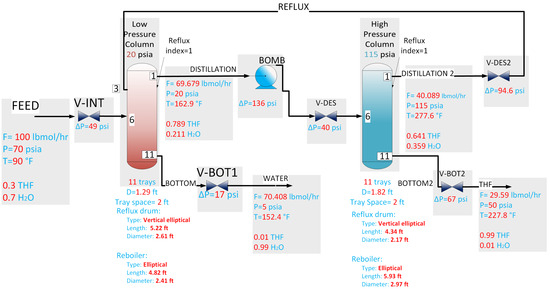
Figure 1. Flow diagram of the azeotropic distillation process with pressure changes.

Several methods exist to separate azeotropic mixtures. One of the simplest methods is to change the pressure of the mixture to shift the azeotrope to a different composition. One of these columns operates near atmospheric pressure to obtain a distillate with a composition close to the azeotropic point. The mixture then enters a second column with a composition close to 0.828 (mole fraction). The second column operates at a much higher pressure. Under these new conditions, the azeotropic point is located at a lower composition than the feed so that the second column operates in a region free of an azeotrope, and it is possible to continue with the purification process. Therefore, the separation can be prolonged until a sufficiently pure product is obtained.

Table 1 shows the geometric parameters of the column, namely, the sizing of the reflux drums, the base of the column, and the diameters of each distillation column. The equipment’s dimensions are necessary for the dynamic simulation. We simulated this process using Aspen Plus V8.0.

Table 1. Sizes of the trays of the columns.

	Low-Pressure Column (14.7 psia)	High-Pressure Column (115 psia)
Diameter (ft)	2.7	1.4
Reflux drum holdup ($f{t}^3$)	28	16
Base holdup ($f{t}^3$)	22	41

The steady-state simulation was developed in the Aspen Plus V8.0 sequential process simulator. The operating conditions and column configuration proposed by Luyben for the case study reported in [33] were considered, corresponding to the process presented in the flow diagram of Figure 1. The pressures were designed to minimize the total annual cost of the separation process. The more significant the difference between the two pressures, the less recycle flow was required and the less energy was consumed. We used the conditions presented before and the sizing of the tanks. The steady-state results defined the process’s nominal conditions, as shown in Table 2. Table 3 presents the nominal values in the steady state for the main flow rates. Finally, Table 4 shows each tray’s temperature and pressure profiles in the steady state in each distillation column.

Table 2. Nominal conditions of the distillation columns.

	Low-Pressure Column (14.7 psia)	High-Pressure Column (115 psia)
Condenser temperature	162.91 °F	277.62 °F
Specific heat of the condenser	−1,889,370 Btu/hr	−1,011,850 Btu/hr
Condenser pressure	20 psia	115 psia
Reflux ratio	1	1
Distillation flow rate	69.66 lbmol/hr	40.07 lbmol/hr
Bottom flow rate	70.41 lbmol/hr	29.59 lbmol/hr
Reboiler temperature	191.99 °F	296.24 °F
Reboiler heat	1,958,810 Btu/hr	1,310,350 Btu/hr
Reboiler pressure	22 psia	117 psia

Table 3. Nominal conditions in the main flow rates.

	Feed Flow Rate	Flow Distillation D1—LPC	Flow Bottom B1—LPC	Flow Distillation D2—HPC	Flow Bottom B2—HPC
Temperature (F)	90	162.9	192	277.6	296.2
Pressure (psia)	70	20	22	115	117
Mass flux (lbmol/hr)	100	69.66	70.41	40.07	29.59
Mass flow rate (lbmol/hr)	3424.27	4228.61	1306.52	2110.95	2117.67
Molar flow composition
THF	30	54.97	0.70	25.68	29.29
Water	70	14.69	69.71	14.39	0.29
Molar fraction composition
THF	0.3	0.78	0.01	0.64	0.99
Water	0.7	0.22	0.99	0.36	0.01

Table 4. Temperature and pressure in each tray in the steady state for both columns. R#EQ1.

	Low-Pressure Column			High-Pressure Column
Stage	Temperature (°F)	Pressure (psia)		Temperature (°F)	Pressure (psia)
1	162.91	20		277.62	115
2	163.50	20.2		277.75	115.2
3	164.20	20.4		277.91	115.4
4	164.77	20.6		278.11	115.6
5	165.42	20.8		278.44	115.8
6	166.81	21		279.03	116
7	167.19	21.2		279.77	116.2
8	167.79	21.4		281.91	116.4
9	168.40	21.6		286.67	116.6
10	169.57	21.8		292.42	116.8
11	191.99	22		296.24	117

We determined the equilibrium liquid–vapor pressure of the THF-H2O mixture using the chemical process simulator Aspen Plus. First, we defined the components and selected the NRTL (non-random two-liquid) thermodynamic property method. Then, we ran a simulation using a Flash unit at atmospheric pressure (14.67 psia). The vapor–liquid equilibrium diagram obtained for the THF–water is shown in Figure 2.

Figure 2. Vapor–liquid equilibrium in the mixture THF-H₂O from Luyben and Chien [34].

The blue curve shows the bubble temperature, while the green curve shows the dew temperature. In a THF–water mixture, when the pressure is constant, the region below the bubble temperature curve represents a liquid mixture, while the region above the dew temperature curve represents a vapor mixture. The area between the two curves indicates the presence of both liquid and vapor phases. At around 0.802 THF composition, the two curves meet at an azeotrope. At this point, the THF composition is the same in both the liquid and vapor phases, making separation impossible under these pressure and temperature conditions [34].

Once the steady-state simulation was completed, the dynamic simulation was performed using Aspen Dynamics v8.0 and Matlab to control the key variables that affect product quality and maintain reduced energy consumption. The plantwide control methodology was used to regulate the plant’s variables; this is described below.

Plantwide Control

Figure 3 shows the general diagram of the control methodology for complete chemical plants. It is a hierarchical methodology that consists of three levels [16]. The first level is optimization. In this, the nominal operating conditions are redefined, establishing a cost function that allows for optimizing aspects such as the energy consumption, production costs, and quantity and quality of the production. The optimization of the process was undertaken in a steady state, respecting the plant design restrictions. The results allow for defining the references for the variables selected in the following levels as controlled variables. The second level is supervision, which consists of defining the primary control of the process that includes the location of the production manipulator to maintain optimal conditions defined by a cost function. Finally, there is the secondary regulation or control level, which ensures the operational conditions of the process.

Figure 3. Hierarchical structure that proposes the Skogestad methodology for the design of a complete plant control structure.

In Figure 3, $C{V}_1$ represents the primary controlled variables, $C{V}_2$ represents the secondary controlled variables, $CV{1}_S$ and $CV{2}_S$ are the references of the controlled variables, d represents the perturbances, $n^y$ are the measured errors, and H and $H_2$ are matrices that represent the controlled variables.

Skogestad’s methodology is divided into 2 parts [16,35]. The steps to follow are described below:

1.

Top-down analysis:

• Definition of operational objectives: determine operational constraints and recognize a scalar cost function J to be minimized and constraints.
• Manipulate variables and degrees of freedom: identify dynamic and steady-state degrees of freedom.
• Self-optimization control: select the primary controlled variables ($C{V}_1$).
• Select the manipulator of throughput: set the production rate.

2.

Bottom-up design:

• Regulatory control layer: the purpose of this layer is to “stabilize” the plant and select “stabilizing” controlled variables ($C{V}_2$).
• Supervisory control layer: control the primary controlled variables.
• Optimization layer: update the setpoints of the primary controlled variables when disturbances occur.

The results and analysis of the methodology applied to the pressure-swing azeotropic distillation columns described before are presented below. First, the steady-state simulation was used in the top-down analysis, and the dynamic simulation was used in the bottom-up design part.

3. Results and Discussion

In this section, the proposed methodology was implemented in the azeotropic distillation plant for the THF-H2O separation process. This was divided into two sections: the first was carried out only with the steady-state simulation of the plant described in the previous section, and the second part describes the controller for the primary and secondary variables that affect the stability, production, and energy consumed by the plant.

1.

Top-Down Analysis

The top-down analysis specifically identified the plant’s primary variables, aiding in formulating the optimization problem. Additionally, constraints were determined.

• Operational objectives and restrictions:
  The objective was to treat the feed rate F₀ = 100 lbmol/hr with a mixture of THF and water. The operational objective was to minimize the energetic cost of this feed rate. In the THF dehydration plant, Equation (1) takes the energy of the reboilers and the recovered energy of the condensers in each column:

  $$J=Q_{reb1}+Q_{reb2}+abs(Q_{cond1}+Q_{cond2})$$

  (1)

  where $Q_{reb1}$ and $Q_{reb2}$ are the reboilers’ energy, and $Q_{cond1}$ and $Q_{cond2}$ are the condensers’ energy in each distillation column.
  We needed to add constraints because the optimization problem requires it. So, the constraints were

  $$F_0=100\mathrm{lbmol}/\mathrm{hr}$$

  (2)

  $$x_{B1,THF}\le 0.01$$

  (3)

  $$x_{B2,THF}\ge 0.99$$

  (4)

  where $x_{B1,THF}$ is the composition of THF in the bottom product of stream B1, $F_0$ is the feed rate of the low-pressure distillation column, and $x_{B1,THF}$ is the composition of THF in the bottom product of stream B2.
• Degrees of freedom analysis:
  We assumed the feed was fixed, so the mode selected was mode 1: given throughput. This corresponded to the standard mode in all the processes.

  (a)

  Identification of the degree of freedom optimization:

  The dynamic degrees of freedom of the systems were

  $$N_m=[F_0,V1,B1,D1,L1,C1,V2,B2,D2,L2,C2]$$

  (5)

  The DOFs in the steady state were obtained by suppressing the tank levels of the dynamics DOFs:

  $$N_{opt}=[F_0,V1,D1,L1,C1,V2,D2,L2,C2]$$

  (6)

  $D_1,$ $D_2,$ $B_1$, and $B_2$ were used by the level controls of $M_{D_1},$ $M_{B_1},$ $M_{D_2}$, and $M_{B_2}$, respectively; these variables did not affect the cost in the steady state of the plant but were controlled to stabilize the plant. Figure 4 represents the process flowsheet with the DOFs analysis.

  

  Figure 4. Process flowsheet with analysis of degrees of freedom in a steady state. The numbers in blue referred to all the DOFs and the red ones to the tank levels.

  (b)

  Identify disturbances in the system:

  We considered the main disturbances in the composition of THF in the feed rate, like (7):

  $$d=\left[z_{F_0}\right]=\left[0.3\pm 0.05THF\right]$$

  (7)

• Self-optimizing control:
  This step presents the selection of the main variables to control to produce the cost function J.

  (a)

  Optimization:

  We defined the primary variables of operation, which were the compositions at the bottom of each column. The products were THF and water with a 0.99 molar fraction. We considered the optimization problem from (2)–(4) and substituted to obtain the following:

  $$minJ\left(u_{ss}\right)=Q_{reb1}+Q_{reb2}+abs(Q_{cond1}+Q_{cond2})$$

  (8)

  $$for{x}_{B1}\le 0.01THF$$

  (9)

  $$for{x}_{B2}\le 0.01H_{2}O$$

  (10)

  Therefore, we resolved this optimization problem using the process simulator Aspen Plus and its tools. Then, we chose the self-optimizing variables. These variables minimized the function J. We included the valves shown in (6). We subtracted three of them: the feed rate because it was an input variable and the vapor generated by the reboilers. After all, they were included in the cost function, and they were dependent on other variables because they are internal streams. Table 5 shows the optimization results, including the bounds and optimal values.

  Table 5. Analysis results of self-optimizing variables.

  Input Variables	Bounds (min/max)	Nominal Value	Optimal Value
  Pressure in high-pressure column	110/120 psia	115 psia	120 psia
  Reflux ratio in high-pressure column	0.2/1.5	1	0.40722
  Pressure in low-pressure column	15/25 psia	20 psia	15 psia
  Reflux ratio in low-pressure column	0.1/1.5	1	0.152835

  Table 5. Analysis results of self-optimizing variables.

  Input Variables	Bounds (min/max)	Nominal Value	Optimal Value
  Pressure in high-pressure column	110/120 psia	115 psia	120 psia
  Reflux ratio in high-pressure column	0.2/1.5	1	0.40722
  Pressure in low-pressure column	15/25 psia	20 psia	15 psia
  Reflux ratio in low-pressure column	0.1/1.5	1	0.152835

  Then, we used the optimal values for these variables in the simulation, and the optimization resulted in a 30% decrease in energy consumption using (1). The energy value was 6.4 × 10⁶ Btu/hr, and the result after optimization was 4.3 × 10⁶ Btu/hr, i.e., a decrease. The most important operating conditions used in the optimization are summarized in the following Table 6.

  Table 6. Operational conditions of the distillation columns after the optimization.

  	Low-Pressure Column (15 psia)	High-Pressure Column (120 psia)
  Condenser temperature	147.50 °F	280.95 °F
  Specific heat of the condenser	−1,119,441.74 Btu/hr	−719,801 Btu/hr
  Condenser pressure	15 psia	120 psia
  Reflux ratio	0.152835	0.40722
  Distillation flow rate	70.60 lbmol/hr	41.00 lbmol/hr
  Bottom flow rate	70.41 lbmol/hr	29.59 lbmol/hr
  Reboiler temperature	179.48 °F	300.03 °F
  Reboiler heat	1,132,014.03 Btu/hr	1,069,961.97 Btu/hr
  Reboiler pressure	17 psia	122 psia

  Table 6. Operational conditions of the distillation columns after the optimization.

  	Low-Pressure Column (15 psia)	High-Pressure Column (120 psia)
  Condenser temperature	147.50 °F	280.95 °F
  Specific heat of the condenser	−1,119,441.74 Btu/hr	−719,801 Btu/hr
  Condenser pressure	15 psia	120 psia
  Reflux ratio	0.152835	0.40722
  Distillation flow rate	70.60 lbmol/hr	41.00 lbmol/hr
  Bottom flow rate	70.41 lbmol/hr	29.59 lbmol/hr
  Reboiler temperature	179.48 °F	300.03 °F
  Reboiler heat	1,132,014.03 Btu/hr	1,069,961.97 Btu/hr
  Reboiler pressure	17 psia	122 psia

  The optimized conditions in the main flow rates are shown in Table 7; the main differences were in the pressures and temperatures, except in the feed flow rate because it was the manipulator of the throughput.

  Table 7. Optimal conditions in the main flow rates.

  	Feed Flow Rate	Flow Distillation D1—LPC	Flow Bottom B1—LPC	Flow Distillation D2—HPC	Flow Bottom B2—HPC
  Temperature (°F)	90	147.502	179.481	280.952	300.037
  Pressure (psia)	70	15	17	120	122
  Mass flux (lbmol/hr)	100	70.571	70.408	40.977	29.593
  Mass flow rate (lbmol/hr)	3424.28	4298.45	1306.51	2180.53	2117.92
  Molar flow composition
  THF	30	55.962	0.704	26.664	29.297
  Water	70	14.609	69.704	14.313	0.296
  Molar fraction composition
  THF	0.3	0.793	0.01	0.650	0.99
  Water	0.7	0.207	0.99	0.349	0.01

  Table 7. Optimal conditions in the main flow rates.

  	Feed Flow Rate	Flow Distillation D1—LPC	Flow Bottom B1—LPC	Flow Distillation D2—HPC	Flow Bottom B2—HPC
  Temperature (°F)	90	147.502	179.481	280.952	300.037
  Pressure (psia)	70	15	17	120	122
  Mass flux (lbmol/hr)	100	70.571	70.408	40.977	29.593
  Mass flow rate (lbmol/hr)	3424.28	4298.45	1306.51	2180.53	2117.92
  Molar flow composition
  THF	30	55.962	0.704	26.664	29.297
  Water	70	14.609	69.704	14.313	0.296
  Molar fraction composition
  THF	0.3	0.793	0.01	0.650	0.99
  Water	0.7	0.207	0.99	0.349	0.01

  Other changes that occurred in the optimization were the profile temperatures of both distillation columns; these changes are presented in Table 8. The differences in the profiles of the temperatures were due to the changes in the operational pressures of both columns. In the LPC, the pressure was lower, so the temperatures dropped. In the HPC, the operating pressure was higher, so the temperatures in the trays rose.

  Table 8. Temperature and pressure after optimization in both columns.

  	Low-Pressure Column			High-Pressure Column
  Stage	Temperature (°F)	Pressure (psia)		Temperature (°F)	Pressure (psia)
  1	147.502	15		280.952	120
  2	148.516	15.2		281.203	120.2
  3	149.591	15.4		281.567	120.4
  4	150.295	15.6		281.965	120.6
  5	151.084	15.8		282.331	120.8
  6	152.590	16		282.636	121
  7	153.245	16.2		283.494	121.2
  8	153.895	16.4		285.812	121.4
  9	154.555	16.6		290.616	121.6
  10	155.728	16.8		296.260	121.8
  11	179.481	17		300.037	122

  Table 8. Temperature and pressure after optimization in both columns.

  	Low-Pressure Column			High-Pressure Column
  Stage	Temperature (°F)	Pressure (psia)		Temperature (°F)	Pressure (psia)
  1	147.502	15		280.952	120
  2	148.516	15.2		281.203	120.2
  3	149.591	15.4		281.567	120.4
  4	150.295	15.6		281.965	120.6
  5	151.084	15.8		282.331	120.8
  6	152.590	16		282.636	121
  7	153.245	16.2		283.494	121.2
  8	153.895	16.4		285.812	121.4
  9	154.555	16.6		290.616	121.6
  10	155.728	16.8		296.260	121.8
  11	179.481	17		300.037	122

  After the optimization, the primary controlled variables were selected using a loss function.

  (b)

  Selection of self-optimizing variables:

  We realized an evaluation to obtain the self-optimizing variables. In this research, we used the “brute force” approach. This approach needed several dynamics simulations. Then, the optimization helped us to find a better energy consumption and simulation in the steady state, so we exported the simulation to a dynamic state using the simulators Aspen Plus and Aspen Plus Dynamics. Figure 5 shows the behavior of the energy consumption when a disturbance in the THF composition was considered.

  

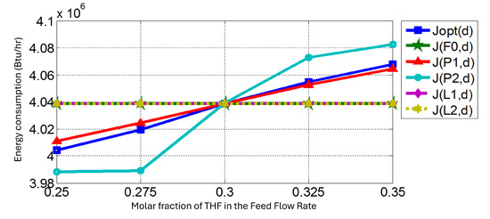  Figure 5. Behavior of the J function when a composition disturbance was considered.

  Figure 5 links the energy consumption in the function to the applied disturbance in the THF composition in the feed rate. The quantification of error concerning the energy in the nominal systems was measured in two ways: with Equation (11), or the loss function, and with the ITAE criterion:

  $$L=J(u_{ss},d)-J_{opt}\left(d\right)$$

  (11)

  where $J_{opt}\left(d\right)$ is the energy consumption value with the disturbances at the molar fraction of the THF in the feed flow rate without controlling any variable. $J(u_{ss},d)$ represents the energy consumption using a variable constant $u_{ss}$. The control of $u_{ss}$ was necessary, while the others did not require control.

  Table 9 shows the results for this analysis, where the primary variables controlled were the compositions at the bottom and the pressure in the low-pressure column. The first set maintained the production objective (the quality of products), and the second set maintained the conditions of optimal energy consumption.

  Table 9. Evaluations of loss and ITAE for candidate variables.

  Constant Variable	Loss Function	ITAE Criterion
  Feed rate	1575.44	733.73
  Pressure in low-pressure column	1214.88	120.55
  Pressure in high-pressure column	−2634.59	590.16
  Reflux ratio in low-pressure column	1575.44	733.72
  Reflux ratio in high-pressure column	1575.44	733.72

  Table 9. Evaluations of loss and ITAE for candidate variables.

  Constant Variable	Loss Function	ITAE Criterion
  Feed rate	1575.44	733.73
  Pressure in low-pressure column	1214.88	120.55
  Pressure in high-pressure column	−2634.59	590.16
  Reflux ratio in low-pressure column	1575.44	733.72
  Reflux ratio in high-pressure column	1575.44	733.72

• Selection of the manipulator of the throughput:
  By default, in the chemical process, the manipulator of the throughput was collocated in the plant’s feed rate.

2.

Bottom-Up Design

The bottom-up analysis focused on the dynamic control of the process. A dynamic process model was needed to validate the implementation of the proposed controlled variables from the top-down analysis. In this part, we first selected the stabilizing controlled variables (CV2) and paired them with the properly manipulated variables (MVs). Then, we determined the structure of the supervisory control layer by pairing the primary CV1 with the remaining manipulated variables.

• Regulation level:
  This section’s main purpose was to maintain the process at acceptable values in the presence of disturbances. We used simple PID controllers. At this point, we needed to make decisions:

  (a)

  Select the secondary controlled variables.

  (b)

  Choose the links between the manipulated and controlled variables, i.e., the closed loops.

  First, we controlled the stabilization in the process. The variables that stabilized the process influenced the mass balance. These variables were the levels and pressures.
  We needed to control the tank level in each distillation column and the pressure in the high-pressure column. Therefore, we controlled the manipulator of the throughput (feedrate) to help maintain the production.
  In Figure 6, the structure regulation control is shown. It had flow control, four-level control, and one pressure control. The controllers stabilized the plant at the regulatory level.
  The controller gains used were empiric values from [33]. Subsequently, they were tuned using Ziegler–Nichols methods. Table 10 presents the configuration of the secondary variables.

  

  Figure 6. Architecture regulation control for the distillation azeotropic process, where FC represents the feed flow rate control; LC1, LC2, LC3, and LC4 represent the level controls in the reflux and reboiler tanks; and PC2 represents the pressure control in the HPC.

  Table 10. Configuration of secondary variable gains using Ziegler–Nichols tuning.

  Controlled Variable	Manipulated Variable	Proportional Gain	Integral Gain	Controller Action
  Feed rate	Valve V1	0.59	0.87	Inverse
  Reflux tank level ${\displaystyle M_{D1}}$	Valve V2	6.57	4.13	Direct
  Reflux tank level ${\displaystyle M_{D2}}$	Valve V4	51.74	2.13	Direct
  Reboiler tank level ${\displaystyle M_{B1}}$	Valve V3	23.34	4.04	Direct
  Reboiler tank level ${\displaystyle M_{B2}}$	Valve V5	6.17	2.53	Direct
  Pressure in the high-pressure column	Heat input in condenser	2	10	Inverse

  Table 10. Configuration of secondary variable gains using Ziegler–Nichols tuning.

  Controlled Variable	Manipulated Variable	Proportional Gain	Integral Gain	Controller Action
  Feed rate	Valve V1	0.59	0.87	Inverse
  Reflux tank level ${\displaystyle M_{D1}}$	Valve V2	6.57	4.13	Direct
  Reflux tank level ${\displaystyle M_{D2}}$	Valve V4	51.74	2.13	Direct
  Reboiler tank level ${\displaystyle M_{B1}}$	Valve V3	23.34	4.04	Direct
  Reboiler tank level ${\displaystyle M_{B2}}$	Valve V5	6.17	2.53	Direct
  Pressure in the high-pressure column	Heat input in condenser	2	10	Inverse

  Figure 7 shows the behavior of the level controls when a change in the setpoints was realized. PI controllers were tuned using the Ziegler–Nichols method. The control signal in each subfigure was the valve opening (represented as a percentage).
  The pressure control in the HPC was regulated using the heat duty condenser. Figure 8 shows the behavior of the pressure control tuned using the Ziegler–Nichols method when we used different setpoints and the control signal behavior.
  Note that in the regulatory control, we did not mention the pressure control for the LPC because it was a primary controlled variable that affected the operational objective.

  

  Figure 7. Level controllers for the regulatory control. PI controls were synchronized using Ziegler–Nichols methods. (a) The reflux tank level $M_{D1}$ control using valve V2. (b) The reflux tank level $M_{D2}$ control using valve V4. (c) The reboiler tank level $M_{B1}$ control using valve V3. (d) The reboiler tank level $M_{B2}$ control using valve V5.

  

  Figure 8. Pressure control for the high-pressure column using the Ziegler–Nichols tuning method.
• Supervisory control:

This stage was responsible for controlling the primary variables of the distillation process. In our case study, these were the concentrations and pressures of the low-pressure column. The supervisory control configuration was divided into three sections.

First, a sensitivity analysis was carried out that allowed for the pairings of variables to be established to define the control loops; that is, the pairs of the controlled output variables and manipulated input variables were determined. Furthermore, their interactions were analyzed. Second, it was decided to indirectly control the compositions of the products with the control of the plate temperatures in the columns. However, it was crucial to properly select a tray to control the temperature in each distillation column. Third, it was decided to design an MPC controller due to the interactions that typically exist in distillation columns. However, the design of a MIMO control was primarily based on the results of the sensitivity analysis. The formulation of a reduced dynamic model of the system was necessary to design the MIMO controller. The system identification technique in state space was used to obtain the mathematical model.

(a)

Sensibility analysis:

This analysis determined the control architecture of the primary controlled variables. For this study, we used the parametric sensitivity formula from [36] with a little modification:

$$S={\displaystyle \frac{\%\Delta \widehat{M}V}{\%\Delta MV}}$$

(12)

where $\Delta \widehat{M}V$ is the variation in the measured variable and $\Delta MV$ is the variation in the manipulated variable. When the sensitivity index S takes values around one, there is a direct relationship between the changes; close to zero, there is no relationship between the variables; and when it is much higher than one, we have an output that is very sensitive to changes in the input. Table 11 presents the values that resulted from this analysis.

Table 11. Results of the sensitivity analysis carried out for the primary variables of the process.

				Output Variables
				THF LPC			THF HPC			Pressure LPC
Input Variables	Nominal Values	Variation of +−5%	Units	Results	% Variation	Sens. Index	Results	% Variation	Sens. Index	Results	% Variation	Sens. Index
HPC reboiler	1,069,696.92	1,123,181.77	Btu/hr	0.85	14.21	2.84	0.99	1.00	0.20	29.61	97.44	19.48
heat		1,016,212.08		0.99	0.23	0.047	0.97	1.42	0.28	12.28	18.09	3.61
HPC reflux	888.3	932.72	lbmol/hr	0.97	3.34	0.67	0.99	0.44	0.08	19.32	28.83	5.76
		843.89		0.93	5.96	1.19	0.99	0.73	0.14	21.72	44.86	8.97
LPC specific	−1,119,431.65	−1,175,403.23	Btu/hr	1.00	1.01	0.20	0.97	1.06	0.21	4.50	69.95	13.99
heat condenser		−1,063,460.06		0.82	17.34	3.47	0.99	1.00	0.20	37.10	147.34	29.46
LPC reboiler	1,127,708.65	1,184,094.08	Btu/hr	0.82	17.29	3.47	0.99	1.00	0.20	46.35	209.03	41.80
heat		1,071,323.21		0.93	5.50	1.10	0.99	0.73	0.14	21.14	40.98	8.19
LPC reflux	657.03	689.88	lbmol/hr	0.81	17.87	3.57	0.99	1.00	0.20	29.46	96.41	19.28
		624.18		0.94	4.62	0.92	0.99	0.62	0.12	20.54	36.96	7.39

With the results reported in Table 11, it could be concluded that the compositions of the bottom products had strong interactions with more than one variable. Therefore, it was decided to implement a MIMO MPC controller to control these primary variables and a PI controller to control the pressure of the low-pressure column (LPC).

One of the ways to control the composition is to do it indirectly to avoid the need to measure the composition. Temperature control was performed instead of a composition control. For this indirect control to work correctly, a constant reflux relationship must be maintained in the process [37]. Therefore, it was necessary to regulate the reflux relations, and to do so, the following was undertaken: To keep the reflux ratio (RR) constant, the Aspen Plus Dynamics simulator used a block called Multiply that maintained the relationship between two inputs and one output. The two inputs were the total distillate mass flow rate of the low-pressure column and the RR value of 0.40722, and the output was the reflux mass flow rate of the low-pressure column. The high-pressure column had the same inlets and outlets, but with an RR of 0.152835.

Figure 9 shows the process flow diagram incorporating these controllers within the simulator. The controllers used to maintain constant reflux are indicated by RR1 and RR2. This regulation allowed the composition to be controlled indirectly by regulating the temperature in a dish.

Figure 9. Flow diagram of the distillation process with changes in pressure, with the reflux controllers presented as RR1 and RR2.

Once this was done, the manipulated variables were reduced to the following: heat in the reboiler of the low- and high-pressure columns and the specific heat of the condenser of the low-pressure column. The last variable was matched to the pressure of the low-pressure column. In summary, the two primary loops consisted of an SISO control to regulate the pressure of the first column to manipulate the heat in the condenser and an MIMO control to regulate the temperature in a plate for each column to manipulate the heat of the reboilers of both columns. The first primary control loop used a PI controller, while the second was developed using an MIMO MPC. However, we needed to know which tray needed to be controlled.

(b)

Temperature control tray selection:

The tray control temperature was selected using the criteria described in Luyben [38]. Figure 10 shows the nominal values of the temperatures in the trays of each column in the Figure 10a,b. These profiles were used in each criterion:

Figure 10. Profiles of the temperatures and temperature slope criteria in the distillation columns.

(i)

Slope criterion: The tray was selected with a significant temperature change from tray to tray. This was the difference between adjacent plates $T_{(n+1)}-T_n$. The Figure 10c,d show this criterion, where we observed the drastic change in the 11th tray in the LP column and a big difference from the 8th to the 9th trays.

(ii)

Sensitivity criterion: A tray was selected where the temperature difference was greater when the manipulated variable changes were sought. This change was suggested to be very small (0.1%), for example, in the heat of the reboiler of each column. Figure 11 shows this criterion. Figure 11a shows the sensitivity in the LP column, which resulted in the 11th plate having the most sensitivity. Figure 11b shows the sensitivity in the HP column, showing that the most sensitive was the ninth plate.

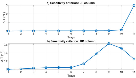Figure 11. Temperature sensitivity criteria in distillation columns.

(iii)

SVD criterion: Singular value decomposition (SVD) analysis was used. A standard SVD program (the MATLAB $svd$ function) decomposed the gain matrix $K^{\prime }$, with the dimensions determined by the number of trays and manipulated variables, rows, and columns. Figure 12 shows the U matrix; this represents the singular values when the reboiler heat changed at several occasions and measured the temperatures in the trays. The results show that the 11th tray in the LP column and the 9th tray in the HP column were the best options to control.

Figure 12. Singular–value decomposed criteria in distillation columns.

(iv)

Invariant temperature criterion: With the bottom and distillate purities fixed, the composition of the feed was manipulated over an expected range. The dish was selected where the temperature did not change despite the changes.

(v)

Minimum product variation criterion: the dish that produced the slightest change in the product purity was chosen, that is, when the purity of the product remained constant, even in the face of disturbances in the feed compositions.

Below, we present the three criteria results, showing that the 11th and 9th plates were chosen to control the temperature in each column.

With the previous results, the temperature of the 11th plate was controlled in the LPC, and the temperature of the 9th plate in the HPC. Once the plates were correctly selected, we used the identification method to identify a model.

(c)

Obtaining an identified model:

The identification systems methodology described in Luyben [33] was used to create a state-space model that represented the behaviors of the reboilers and the temperatures of the trays, i.e., the 11th tray in the HP column and the 9th tray in the LP column.

First, an experiment to acquire data was designed using a PRBS signal with 6 bits; the amplitudes of the signals was given for the low-pressure column as $1.12\times {10}^6\pm 1$% Btu/hr, and the high-pressure column as $1.06\times {10}^6\pm 1.54$% Btu/hr, with a total duration of 94.5 h. These input signals are shown in Figure 13. Figure 14 shows the temperatures of the selected trays.

Figure 13. PRBS input signals for system model identification.

Figure 14. Measured system outputs when the input was the PRBS signal.

Using the inputs–output data, we systematically created different models that accurately represented the data’s behavior. We found a robust state-space model using the system identification toolbox in this case. To determine the best model that gave the best estimation of the measured data, we assessed the normalized root-mean-square error (NRMSE) Equation (13) and searched for the maximum FIT; the state-space model is presented in Equation (14), which reached above 95% of FIT. The results are shown in Figure 15.

$$FIT=100\left(1-∥{\displaystyle \frac{y-\widehat{y}}{y-\overline{y}}}∥\right)$$

(13)

$$\begin{array}{cc}x(k+1)=& Ax\left(k\right)+Bu\left(k\right)\\ y\left(k\right)=& Cx\left(k\right)\end{array}$$

(14)

where

$$\begin{array}{l}A=\left[\begin{array}{cccc}-18.12& -1.202& 0.7138& 5.527\\ 22.2& -7.919& -12.79& -3.178\\ -0.5539& 0.3601& 0.07509& -0.7253\\ -14.71& -2.306& 2.691& 1.376\end{array}\right],\hfill \\ B=\left[\begin{array}{cc}-0.0006884& 0.0003937\\ 0.001389& -0.0008602\\ -0.00004811& 0.00002849\\ -0.0005596& 0.0003121\end{array}\right],\\ C=\left[\begin{array}{cccc}-24.84& -4.272& -56.92& 18.68\\ -10.66& 4.655& -6.074& -0.0803\end{array}\right]\end{array}$$

(15)

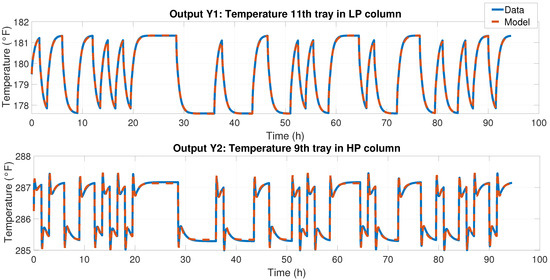Figure 15. Comparison of the experiment data vs. the model identified in the state space; for output Y1, the fit achieved was 98.04%, and for output Y2, the fit achieved was 93.75%.

We obtained a 2 × 2 MIMO model, i.e., a model with two inputs and two outputs, as described in Equations (14) and (15). Once the identified model was obtained, we designed an MIMO MPC controller.

(d)

Designing the MPC controller:

The model represented in Equation (14) predicted the dynamics of the THF dehydration process. The MPC controller was configured and implemented in Simulink/MATLAB 2023a using the Model Predictive Control toolbox. A discrete state-space model was first used to design the controller.

The constraints for the manipulated variables were set as two minimum values and two maximum values. The minimum values were the nominal values in a steady state of the heat of the reboilers in each distillation column. In contrast, the amount of heat determined the maximum values that the process supported without generating losses greater than 5 lbmol/hr in the flow of the THF product when various perturbations were applied. Regarding the restrictions of the controlled variables, no limit was set.

In the LP column, the heat reboiler constraints were from $1.1052\times {10}^6$ to $1.1503\times {10}^6$ Btu/hr, and in the HP column, the constraints in the heat reboiler were from $1.0483\times {10}^6$ to $1.0911\times {10}^6$ Btu/hr. The complete plantwide schematic with the regulatory and supervisory controls is presented in Figure 16.

Figure 16. Process flow diagram with controllers for secondary controlled variables and MPC for primary controlled variables.

The primary controls used a PI controller to maintain the 15 psia pressure in the LPC and the MIMO MPC, with the plates’ temperatures as the measured outputs and the heat reboilers as the manipulated variables. The pressure control maintained the operational objectives, and the MPC maintained the production objective. Table 12 describes these controllers and parameters.

Table 12. Configuration of primary controllers in the supervisory stage.

Type of Control	SISO PI	MIMO MPC
Controlled variable	Pressure in LPC	Temperatures: Tray 11 in LPC Tray 9 in HPC
Manipulated variable	Heat duty in condenser in LPC	Heat reboiler in each column
Model	PI Proportional gain: 6.17 Integral gain: 2.53	MIMO (2 × 2 system) described in Equation (14)
Controller action	Inverse	—
Parameters MPC
Prediction horizon		75
Control horizon		50
Cost function		$J={\sum }_{k=0}^P\left({∥y_{ref}\left(k\right)-y\left(k\right)∥}_Q^2+{∥\Delta u\left(k\right)∥}_R^2\right)$
Weights		R = 1500, Q = 800
Constraints		Qreb in LPC Min: $1.12\times {10}^6$ Max: $1.40\times {10}^6$ Qreb in HPC Min: $1.06\times {10}^6$ Max: $1.35\times {10}^6$

The MPC controller regulated and supervised the purity of the product at the bottom. Figure 17 presents the controller’s behavior with disturbances presented in terms of the molar fraction of the feed flow rate. The temperature in the ninth tray of the HPC aimed to be above the nominal value of 290.83 °F; when the disturbance was high, i.e., more than a 0.325 molar fraction, we observed that the temperature dropped a few degrees above the nominal temperature. The purity in all the cases maintained the 0.99 molar fractions or above, except at times 1, 4, and 7 h. One possible reason was that we had a slow process because we manipulated the temperature to control the purities and stabilize the signal. The control needed more time, and these intervals were short compared with the stabilizing time of the plant (about 1.5 h).

Figure 17. Behavior of the manipulated variable and product purity with disturbances in the feed flow rate. (a) A disturbance in the THF molar fraction in the feed. (b) The temperature of the 9th tray in the HPC. (c) The purity of the bottom product in the HPC.

The main objective in the supervision stage was to measure the energy consumption by the reboilers; for this, a test was carried out against disturbances in the concentration of the THF inlet flow. We compared the plantwide structure from Luyben [33] and our proposal.

The test carried out was as follows: a step perturbation was applied after one hour of simulation; this step generated a change in the mole fraction of THF from 0.3, which was the nominal value, to the following values: 0.25, 0.275, 0.325, and 0.35. The test was carried out for 8 h of simulation, and the last acquired value of the energy consumed by the process was taken. Figure 18 shows the energy consumed by the process in the face of each disturbance, and it was observed that the proposed control structure had a lower energy consumption and remained within the range. In contrast, the structure proposed by Luyben had a linear behavior. On average, the proposed structure consumed 26.95% less when each disturbance was applied.

Figure 18. Comparison of the energy consumption by the plantwide control structures under different perturbations in terms of the concentration of THF in the feed stream. In green is the one proposed by Luyben, and in blue is the one proposed by this research.

Also, the THF molar fraction at the bottom of the HP column was analyzed and the results are presented in Figure 19, where our proposal conserved the 0.99 molar fractions of the products. Instead, Luyben’s method maintained an error.

Figure 19. Comparison of the THF concentrations in the bottom product of the high-pressure column under different disturbances in the feed flow rate.

Among the tests performed, one was performed with a varying amplitude perturbation on the THF concentration in the feed stream, where the amplitude varied between values of 0.25 and 0.35 molar fractions, as presented in the top of Figure 20. The result is that the energy consumed in the event of this perturbation behaved like in the bottom of Figure 20, and the results of the concentration in the bottom product are presented in Figure 21.

Figure 20. (a) Variant amplitude disturbance. (b) The two control structures consumed energy in response to the disturbance. The proposed method consumed less energy than the Luyben method for the disturbance applied.

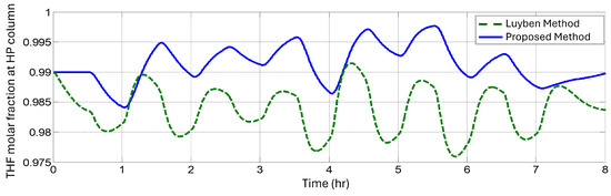
Figure 21. THF concentration in the bottom product of the high-pressure distillation column when the perturbation was applied.

Figure 20 and Figure 21 show that Luyben’s plantwide control consumed 33% more than the proposed plantwide control using the Skogestad methodology. Our work presents a stable energy consumption and maintained, almost all the time, a purity higher than a 0.99 THF molar fraction. In the cases where we maintained a constant disturbance, Figure 19 compares the methodologies and shows the THG molar fraction. It was observed that Luyben’s methodology always remained lower than the desired purity, in contrast with our method, which always aimed to remain higher.

4. Conclusions

Skogestad’s methodology for designing comprehensive plantwide control systems offers significant economic benefits, primarily through maximizing the production efficiency or minimizing the energy consumption. In this study, the optimized control strategy resulted in a dynamic energy consumption reduction of 33% during the disturbances compared with the Luyben structure. This improvement was attributed to the initial minimization of the objective function J in Skogestad’s procedure and the subsequent process reconfiguration based on optimization. The strategy achieved 36% energy savings in steady-state conditions while maintaining nominal feed and bottom product flows.

The supervisory control scheme, a key component of our study, effectively stabilized the energy consumption against variations in the feed flow rates. It also ensured consistent product purity at a 0.99 molar fraction of tetrahydrofuran (THF). This scheme, when implemented, significantly improved the system’s stability and product quality. Additionally, the MIMO MPC system, another important aspect of our study, controlled the reboiler heat and tray temperatures, which contributed to the stable operation and enhanced process efficiency.

Future research will explore alternative local methods for selecting primary controlled variables and investigate advanced control techniques for the MIMO system focusing on heat reboilers and tray temperatures. Additionally, Skogestad’s methodology will be applied to the azeotropic distillation plant prototype at Centro Universitario de Los Valles, providing practical insights and further validating the effectiveness of the proposed control strategies.

References

- López Núñez, A.R.; Rumbo Morales, J.Y.; Salas Villalobos, A.U.; De La Cruz-Soto, J.; Ortiz Torres, G.; Rodríguez Cerda, J.C.; Calixto-Rodriguez, M.; Brizuela Mendoza, J.A.; Aguilar Molina, Y.; Zatarain Durán, O.A.; et al. Optimization and recovery of a pressure swing adsorption process for the purification and production of bioethanol. Fermentation 2022, 8, 293. [Google Scholar] [CrossRef]
- Rumbo Morales, J.Y.; López López, G.; Alvarado, V.M.; Torres Cantero, C.A.; Azcaray Rivera, H.R. Optimal predictive control for a pressure oscillation adsorption process for producing bioethanol. Comput. Sist. 2019, 23, 1593–1617. [Google Scholar]
- Brizuela-Mendoza, J.A.; Sorcia-Vázquez, F.D.; Rumbo-Morales, J.Y.; Ortiz-Torres, G.; Torres-Cantero, C.A.; Juárez, M.A.; Zatarain, O.; Ramos-Martinez, M.; Sarmiento-Bustos, E.; Rodríguez-Cerda, J.C.; et al. Pressure swing adsorption plant for the recovery and production of biohydrogen: Optimization and control. Processes 2023, 11, 2997. [Google Scholar] [CrossRef]
- Rumbo-Morales, J.Y.; Ortiz-Torres, G.; Sarmiento-Bustos, E.; Rosales, A.M.; Calixto-Rodriguez, M.; Sorcia-Vázquez, F.D.; Pérez-Vidal, A.F.; Rodríguez-Cerda, J.C. Purification and production of bio-ethanol through the control of a pressure swing adsorption plant. Energy 2024, 288, 129853. [Google Scholar] [CrossRef]
- Ortiz-Torres, G.; Rumbo-Morales, J.; Sorcia-Vázquez, F.; Pérez-Vidal, A.; Cruz-Rojas, A.; Brizuela-Mendoza, J.; Oceguera-Contreras, E. Concentration estimation and fault tolerant control in a CSTR modelled as a quasi linear parameter varying system. Rev. Mex. Ingeniería Química 2021, 20, 51–66. [Google Scholar] [CrossRef]
- Buckley, P. Techniques of Process Control; John Wiley: New York, NY, USA, 1964. [Google Scholar]
- Ochoa, S.; Wozny, G.; Repke, J.U. Plantwide Optimizing Control of a continuous bioethanol production process. J. Process. Control 2010, 20, 983–998. [Google Scholar] [CrossRef]
- Luyben, W.L. Tuning proportional-integral-derivative controllers for integrator/deadtime processes. Ind. Eng. Chem. Res. 1996, 35, 3480–3483. [Google Scholar] [CrossRef]
- Larsson, T.; Skogestad, S. Plantwide control—A review and a new design procedure. Model. Identif. Control 2000, 21, 209–240. [Google Scholar] [CrossRef]
- Araújo, A.; Skogestad, S. Control structure design for the ammonia synthesis process. Comput. Chem. Eng. 2008, 32, 2920–2932. [Google Scholar] [CrossRef]
- Gera, V.; Kaistha, N.; Panahi, M.; Skogestad, S. Plantwide Control of a Cumene Manufacture Process. Comput. Aided Chem. Eng. 2011, 29, 522–526. [Google Scholar] [CrossRef]
- Panahi, M.; Skogestad, S. Economically efficient operation of CO2 capturing process. Part II. Design of control layer. Chem. Eng. Process. Process. Intensif. 2012, 52, 112–124. [Google Scholar] [CrossRef]
- Jagtap, R.; Kaistha, N.; Skogestad, S. Economic plantwide control over a wide throughput range: A systematic design procedure. AIChE J. 2013, 59, 2407–2426. [Google Scholar] [CrossRef]
- Minasidis, V.; Skogestad, S.; Kaistha, N. Simple Rules for Economic Plantwide Control. In Computer Aided Chemical Engineering; Elsevier: Amsterdam, The Netherlands, 2015. [Google Scholar]
- Skogestad, S. Plantwide control: The search for the self-optimizing control structure. J. Process. Control 2000, 10, 487–507. [Google Scholar] [CrossRef]
- Skogestad, S. Control structure design for complete chemical plants. Comput. Chem. Eng. 2004, 28, 219–234. [Google Scholar] [CrossRef]
- Jahanshahi, E.; Krishnamoorthy, D.; Codas, A.; Foss, B.; Skogestad, S. Plantwide control of an oil production network. Comput. Chem. Eng. 2020, 136, 106765. [Google Scholar] [CrossRef]
- Martínez-Sánchez, O.; Gómez-Castro, F.I.; Ramírez-Corona, N. Plantwide control of a biodiesel production process with variable feedstock. Chem. Eng. Res. Des. 2022, 185, 377–390. [Google Scholar] [CrossRef]
- Gera, V.; Panahi, M.; Skogestad, S.; Kaistha, N. Economic plantwide control of the cumene process. Ind. Eng. Chem. Res. 2013, 52, 830–846. [Google Scholar] [CrossRef]
- Lin, Y.J.; Pan, T.H.; Wong, D.S.H.; Jang, S.S.; Chi, Y.W.; Yeh, C.H. Plantwide Control of CO2 Capture by Absorption and Stripping Using Monoethanolamine Solution. Ind. Eng. Chem. Res. 2011, 50, 1338–1345. [Google Scholar] [CrossRef]
- Ghuge, P.D.; Mali, N.A.; Joshi, S.S. Comparative analysis of extractive and pressure swing distillation for separation of THF-water separation. Comput. Chem. Eng. 2017, 103, 188–200. [Google Scholar] [CrossRef]
- Luyben, W.L. Comparison of flowsheets for THF/water separation using pressure-swing distillation. Comput. Chem. Eng. 2018, 115, 407–411. [Google Scholar] [CrossRef]
- Iqbal, A.; Ahmad, S.A. Entrainer based economical design and plantwide control study for Tetrahydrofuran/Water separation process. Chem. Eng. Res. Des. 2018, 130, 274–283. [Google Scholar] [CrossRef]
- Bartokova, B.; Laredo, T.; Marangoni, A.G.; Pensini, E. Mechanism of tetrahydrofuran separation from water by stearic acid. J. Mol. Liq. 2023, 391, 123262. [Google Scholar] [CrossRef]
- Xu, S.; Bao, J. Plantwide process control with asynchronous sampling and communications. J. Process. Control 2011, 21, 927–948. [Google Scholar] [CrossRef]
- Chapman, P.D.; Tan, X.; Livingston, A.G.; Li, K.; Oliveira, T. Dehydration of tetrahydrofuran by pervaporation using a composite membrane. J. Membr. Sci. 2006, 268, 13–19. [Google Scholar] [CrossRef]
- Yamaki, T.; Matsuda, K.; Huang, K.; Matsumoto, H.; Nakaiwad, M. Separation of Binary mixture using Pressure Swing Distillation with Heat Integration. In Proceedings of the Symposium on Computer Aided Process Engineering, London, UK, 17–20 June 2012; Volume 17, p. 20. [Google Scholar]
- Zhang, Z.g.; Huang, D.h.; Lv, M.; Jia, P.; Sun, D.z.; Li, W.x. Entrainer selection for separating tetrahydrofuran/water azeotropic mixture by extractive distillation. Sep. Purif. Technol. 2014, 122, 73–77. [Google Scholar] [CrossRef]
- Shan, B.; Sun, D.; Zheng, Q.; Zhang, F.; Wang, Y.; Zhu, Z. Dynamic control of the pressure-swing distillation process for THF/ethanol/water separation with and without thermal integration. Sep. Purif. Technol. 2021, 268, 118686. [Google Scholar] [CrossRef]
- Xu, Q.; Liu, X.; Sun, D.; Shan, B.; Cui, P.; Wang, Y.; Zhang, F. Heat integration and dynamic control of reactive pressure-swing distillation for separation of tetrahydrofuran/ethanol/water. Chem. Eng. Process. Process. Intensif. 2023, 191, 109466. [Google Scholar] [CrossRef]
- Mtogo, J.W.; Mugo, G.W.; Mizsey, P. Dynamic Controllability Study of Extractive and Pressure-Swing Distillations for Tetrahydrofuran/Water Separation. Chem. Eng. Technol. 2023, 46, 1706–1716. [Google Scholar] [CrossRef]
- Herslund, P.J.; Thomsen, K.; Abildskov, J.; von Solms, N. Application of the cubic-plus-association (CPA) equation of state to model the fluid phase behaviour of binary mixtures of water and tetrahydrofuran. Fluid Phase Equilibria 2013, 356, 209–222. [Google Scholar] [CrossRef]
- Luyben, W. Plantwide Dynamic Simulators in Chemical Processing and Control; CRC Press: Boca Raton, FL, USA, 2002. [Google Scholar]
- Luyben, W.L.; Chien, I.L. Design and Control of Distillation Systems for Separating Azeotropes; John Wiley & Sons: Hoboken, NJ, USA, 2011. [Google Scholar]
- Downs, J.J.; Skogestad, S. An industrial and academic perspective on plantwide control. Annu. Rev. Control 2011, 35, 99–110. [Google Scholar] [CrossRef]
- Dorf, R.C. Sistemas de Control Moderno; Pearson Educación: London, UK, 2005. [Google Scholar]
- Hori, E.S.; Skogestad, S. Selection of control structure and temperature location for two-product distillation columns. Chem. Eng. Res. Des. 2007, 85, 293–306. [Google Scholar] [CrossRef]
- Luyben, W.L. Control of a multiunit heterogeneous azeotropic distillation process. AIChE J. 2006, 52, 623–637. [Google Scholar] [CrossRef]
Disclaimer/Publisher’s Note: The statements, opinions and data contained in all publications are solely those of the individual author(s) and contributor(s) and not of MDPI and/or the editor(s). MDPI and/or the editor(s) disclaim responsibility for any injury to people or property resulting from any ideas, methods, instructions or products referred to in the content. |
© 2024 by the authors. Licensee MDPI, Basel, Switzerland. This article is an open access article distributed under the terms and conditions of the Creative Commons Attribution (CC BY) license (https://creativecommons.org/licenses/by/4.0/).