Scheduling Jobs on Unreliable Machines Subject to Linear Risk

Abstract

Background: This paper addresses a new class of scheduling problems in the context of machines subject to (unrecoverable) interruptions; i.e., when a machine fails, the current and subsequently scheduled work on that machine is lost. Each job has a certain processing time and a reward that is attained if the job is successfully completed. Methods: For the failure process, we considered the linear risk model, according to which the probability of machine failure is uniform across a certain time horizon. Results: We analyzed both the situation in which the set of jobs is given, and that in which jobs must be selected from a pool of jobs, at a certain selection cost. Conclusions: We characterized the complexity of various problems, showing both hardness results and polynomial algorithms, and pointed out some open problems.

1. Introduction

This paper addresses a scheduling problem that arises in the context of machines subject to failures. In several models, failures imply the temporary unavailability of the machine and they occur at unpredicted times, though a probabilistic description of the failure process is usually available [1]. In many models, after the machine recovers from failure, the job that was being processed can either continue where it left off (preempt-resume models), or it has to be restarted from scratch (preempt-repeat models) [2,3]. In these cases, the problem is to optimize a classical scheduling-related objective, such as the weighted completion time or some tardiness-related measure, etc. In this paper, we address a different situation, namely when machines are subject to unrecoverable interruptions [4]. By “interruption”, we mean that, while processing a job, a processing resource may become unavailable for whatever reason (e.g., a real machine failure or the machine being preempted by some higher-priority user). In any case, when an interruption occurs, the current job and all subsequently scheduled jobs on the machine are lost. In such contexts, we consider that each job has a certain value if successfully carried out, and the problem becomes that of deciding the schedule of the jobs so as to maximize the expected amount of this value. Clearly, such a decision must take into account the specificity of the failure process of the machine(s). The models addressed in this paper have applications in both manufacturing [5] and computer systems [6].

This paper addresses the following scenario. Consider a job set $J=\{1,\dots ,n\}$ ($\left|J\right|=n$) and m identical machines. Each job requires a certain processing time $p_j$, $j=1,\dots ,n$ and, if it is successfully carried out, a reward $r_j$ is gained. The machines are subject to unrecoverable interruptions.

In this context, we address two different problem types:

(i)

Given J, the problem is to assign the jobs to the m machines and sequence them on each machine in order to maximize the expected reward. We called this problem the unrecoverable interruption machine-scheduling problem, and denote it by UIMSP$\left(m\right)$.

(ii)

Given J, for each job, a selection cost $c_j$ is further specified for selecting it. The problem is then to decide which subset $S\subseteq J$ of jobs should be selected, and how the selected jobs should be assigned and sequenced on the machines in order to maximize the net expected reward, i.e., the expected reward of the selected jobs minus their selection cost. The problem is then called the unrecoverable interruption machine-scheduling problem with job selection, denoted by UIMSPS$\left(m\right)$. The cardinality of S may or may not be fixed, giving rise to two variants of the problem. If it is imposed that $\left|S\right|=k$, the problem is denoted by UIMSPS_k(m).

Note that $c_j$ represents the cost to secure job j, e.g., the cost of raw materials or other fixed costs. It is important to underline that, even if a selected job is not carried out because of the interruption, the cost $c_j$ is borne anyhow.

For UIMSP (and UIMSPS) to be fully defined, one must specify the machine failure process. In this paper, we addressed the case in which the failure process follows a linear risk model, i.e., the probability of interruption is proportional to the amount of time elapsed since the beginning of the schedule (see, e.g., [6]). In our paper, we considered that a time horizon of length T is given, i.e., the jobs must be completed within a certain time horizon T, as the machine is not available afterwards. Besides representing all situations with a constant failure rate, the linear risk assumption can conveniently represent situations in which access to the processing resource is given at budget cost, but it is not granted for the whole time horizon, as some higher-priority users may claim the resource at any time [6]. Without any information on when the resource can be withdrawn, we assume that the interruption probability is uniformly distributed across the time horizon, hence yielding the linear risk model.

In this paper, we address various problems:

• UIMSP(1). In this case, we show that the problem can be solved in polynomial time by a simple priority rule.
• UIMSPS(1). We show that UIMSPS_k(1) is, in general, NP-hard, but some special cases are polynomially solvable. We derived a particularly efficient algorithm for the case in which jobs have a unit-processing time ($p_j=1$).
• UIMSP(m). We show that the problem is, in general, NP-hard, but it can be solved in polynomial time for the special case in which all jobs have the same reward ($r_j=r$) or the same processing times ($p_j=p$).

The layout of this paper is as follows. In Section 2, we review the relevant literature on these kinds of problems. In Section 3, the various complexity results are presented. Section 4 reports the results of a set of computational experiments. Finally, in Section 5, some conclusions are drawn.

2. Literature Review

Scheduling models in which machines may fail constitute a meaningful subfield in the area of machine scheduling [1]. However, in most of these models, it is assumed that the machine remains unavailable for a certain time span (during which it is repaired), and thereafter, processing activity can be resumed [2]). Unlike these contexts, here we consider that machine interruptions are unrecoverable, i.e., there is no possibility of resuming jobs that have been interrupted or processing jobs that have not even started. Hence, scheduling decisions must carefully take this issue into account. Unlike usual scheduling settings, the manager’s objectives are not related to classical objective functions such as tardiness or flow time-related measures, but rather to maximizing the expected profit.

Enlarging the view beyond the scheduling domain, there are other situations in which unrecoverable events may bring activities to a halt. For example, in the case of project scheduling, uncontrollable events may force the project to close down [7], or in diagnostic problems, the tests are stopped when the results of the previous tests show that the overall system is not properly working [8]. Within the scheduling field, unrecoverable interruptions are considered in cloud computing, and strategies are enacted to hedge against host permanent failures (HPCs) [9]. Benoit et al. [6] analyzed the problem of sharing the workload among various computers subject to unrecoverable interruptions, using strategies such as job replication or checkpointing. A stream of works exists in which failure probabilities are associated with the jobs; i.e., for each job j, a probability ${\pi }_j$ is given that the machine will fail while performing that job. This problem is called the unreliable job-scheduling problem (UJSP). The problem is to sequence the jobs in order to maximize the expected reward. Under a different name, this problem was introduced by Stadje [10], who was the first to show that a simple priority rule solves UJSP without further constraints. For $m=2$, UJSP becomes NP-hard [5], and a list-scheduling algorithm on m machines produces a solution that is $0.8535$-approximate [11]. Notice that, if the machine failure process is exponentially distributed, the probability that a job is successfully carried out does not depend on the amount of time elapsed, but only on the job’s processing time. In this case, if $p_j$ denotes the processing time of job j, then ${\pi }_j=e^{-\lambda p_j}$. In other words, when machine failures are exponentially distributed, UJSP and UIMSP coincide. This special case of UJSP is dealt with in [12]. We are not aware of papers that have addressed UIMSP with linear risks, but in [13], the need for investigating this type of failure model is pointed out.

The selection variant of UJSP has received less attention in the literature; however, it has been shown [10] that the problem of selecting the jobs in order to maximize the net expected reward can be solved by a greedy algorithm when all the jobs have the same selection cost. Ref. [14] further characterized special cases of selection problems (including UJSP), which can be solved by a greedy approach. However, in the previous papers, the complexity of the general UJSP with selection costs was left open. We are not aware of papers that have addressed UIMSP with job selection (i.e., UIMSPS). Our paper, using a linear risk model, is the first contribution in this sense.

3. Methodology

In this section, we address the complexity of various cases of UIMSP and UIMSPS when failures follow a linear risk model. Under this model, a time horizon T is specified, and the failure probability is uniformly distributed across T. Hence, the probability that a machine is still working at time $t<T$, which can be called $q_t$, is given by

$$q_t=1-{\displaystyle \frac{t}{T}}.$$

(1)

When $m\ge 2$, machines may fail independently, and the time horizon T is the same for each machine.

In the following, if $T\ge {\sum }_i{p}_i$, we say that T is nonbinding; otherwise, we say that T is binding.

3.1. UIMSP(1)

Let us start from the simplest problem, i.e., there is a single machine and there are no selection costs. In what follows, we consider the case when T is nonbinding.

Given a schedule $\sigma$, let $\sigma \left(i\right)$ denote the job in the i-th position. So, the first scheduled job is $\sigma \left(1\right)$, of length $p_{\sigma \left(1\right)}$ and reward $r_{\sigma \left(1\right)}$. Due to (1), the expected reward stemming from the execution of the first scheduled job is given by

$$r_{\sigma \left(1\right)}\left(1-{\displaystyle \frac{p_{\sigma \left(1\right)}}{T}}\right).$$

The reward of $\sigma \left(2\right)$ is attained if the machine does not fail within time $p_{\sigma \left(1\right)}+p_{\sigma \left(2\right)}$; hence, its contribution to the expected reward is

$$r_{\sigma \left(2\right)}\left(1-{\displaystyle \frac{p_{\sigma \left(1\right)}+p_{\sigma \left(2\right)}}{T}}\right),$$

and so on. Given a schedule $\sigma =\left\{\sigma \right(1),\sigma (2),\dots ,\sigma \left(n\right)\}$, the expected reward $ER\left(\sigma \right)$ of the schedule $\sigma$ is therefore given by

$$ER\left(\sigma \right)=\sum _{i=1}^n{r}_{\sigma \left(i\right)}\left(1-{\displaystyle \frac{{\sum }_{k=1}^i{p}_{\sigma \left(k\right)}}{T}}\right).$$

(2)

Example 1.

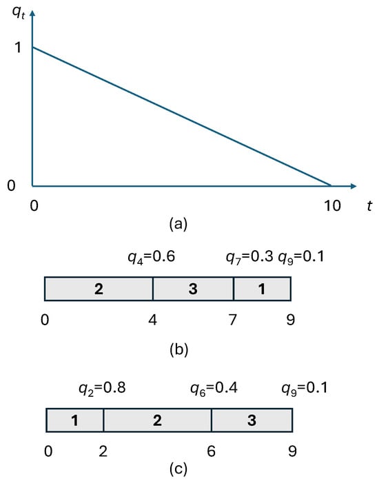
Consider the example in Table 1, where $T=10$. Figure 1a shows the probability $q_t$ that the machine is still working at time t. Starting from 1, $q_t$ linearly decreases, becoming 0 at time $T=10$. Figure 1b illustrates a feasible schedule $\{2,3,1\}$. Under this schedule, the probability of successfully carrying out job 2 is $(1-p_2/T)=0.6$; hence, the expected reward from scheduling job 2 is $r_2(1-p_2/T)=80·0.6=48$. The probability of successfully carrying out job 3 is $(1-(p_2+p_3)/T)=0.3$, and therefore, job 3 contributes by $r_3(1-(p_2+p_3)/T)=55·0.3=16.5$. A similar computation for job 1 yields $r_1(1-(p_2+p_3+p_1)/T)=50·0.1=5$; hence, the total expected reward of this schedule is $z=69.5$.

Table 1. Data for Example 1.

i	1	2	3
$p_i$	2	4	3
$r_i$	50	80	55
$p_i/r_i$	0.04	0.05	0.0545

Figure 1. The linear risk function (a) and two feasible schedules (b) and (c) for Example 1.

We next show that UIMSP(1) can be efficiently solved when T is nonbinding. From (2), we have

$$ER\left(\sigma \right)=\sum _{i=1}^n{r}_{\sigma \left(i\right)}-{\displaystyle \frac{1}{T}}\sum _{i=1}^n{r}_{\sigma \left(i\right)}\left(\sum _{h=1}^i{p}_{\sigma \left(h\right)}\right).$$

(3)

Since the first term of the above expression is a constant, the expected reward $ER\left(\sigma \right)$ is maximized when

$${\displaystyle \frac{1}{T}}\sum _{i=1}^n{r}_{\sigma \left(i\right)}\left(\sum _{h=1}^i{p}_{\sigma \left(h\right)}\right)$$

(4)

is minimized. Now consider the classical scheduling problem $1\left|\right|\sum w_j{C}_j$, consisting of minimizing the total weighted completion time of n jobs, with each having a processing time $p_j$ and a weight $w_j$. If we let $w_j:=r_j/T$, observing that $p_{\sigma \left(1\right)}+\dots ,p_{\sigma \left(i\right)}$ is the completion time of the job in the i-th position, (4) coincides with the value of the total weighted completion time of a given schedule. As a consequence, (4) is minimized by sequencing the jobs according to Smith’s rule [15], i.e., by nondecreasing order of the ratios

$${\displaystyle \frac{p_j}{r_j}}.$$

(5)

Theorem 1.

When $m=1$, UIMSP under linear risk is solved in $O(nlogn)$.

Note that the ordering rule is fairly intuitive, in that it gives precedence to jobs with a small processing time and a large reward.

Example 2.

By sequencing the jobs of Example 1 by increasing ratios $p_j/r_j$, one obtains the schedule in Figure 1c, i.e., schedule $\{1,2,3\}$. This is the optimal schedule, and its value is given by $50(1-2/10)+80(1-(2+4)/10)+55(1-(2+4+3)/10)=77.5$.

Finally, we observe that, if T is binding (i.e., $T<{\sum }_j{p}_j$), the nature of the problem changes significantly, since no jobs can complete after T. Thus, the problem becomes deciding which jobs should be completed before T, and UIMSP(1) becomes equivalent to UIMSPS(1) with no costs. The complexity of UIMSP(1) in this case is still open.

3.2. UIMSPS(1) and UIMSPS_k(1)

In this section, we address the problem with selection costs; i.e., each job j also has a cost $c_j$ that is paid if the job is selected for processing. Notice that, once a subset $S\subseteq J$ of jobs is selected to be performed within T, the optimal sequence is obtained by ordering the jobs according to (5). Hence, UIMSPS(1) essentially consists of finding S. In what follows, we denote by $z\left(S\right)$ the value of the net expected reward when S is selected, i.e., from (2):

$$z\left(S\right)=ER\left(S\right)-\sum _{j\in S}{c}_j$$

(6)

We next propose a dynamic programming algorithm for solving UIMSPS(1). In what follows, we assume that the jobs are numbered by nondecreasing values of the ratio (5). For a given positive integer $B\le T$, let $\mathcal{P}(j,B)$ denote the subproblem restricted to jobs $\{1,2,\dots ,j\}$, under the condition that the last selected job completes exactly at time B. We denote by $F(j,B)$ the value of the optimal solution of $\mathcal{P}(j,B)$. It is possible to express $F(j,B)$ by means of the following recursive formula:

$$F(j,B)=max\{F(j-1,B);F(j-1,B-p_j)+r_j(1-{\displaystyle \frac{B}{T}})-c_j\}$$

(7)

The first term corresponds to the case in which j is not selected in the optimal solution of $\mathcal{P}(j,B)$. The second term corresponds to selecting j, in which case job j is appended at the end of the optimal solution of $\mathcal{P}(j,B-p_j)$, and the contribution of job j is accounted for. The value of the optimal solution of UIMSPS(1) is given by

$$z^{*}=\underset{0\le B\le T}{max}\left\{F(n,B)\right\}.$$

(8)

The correctness of the algorithm is derived from the following considerations. Suppose that, for some $(j,B)$, in the optimal solution of $\mathcal{P}(j,B)$, there is some idle time of length $\tilde{I}$ between two consecutive jobs (which is possible, to meet the constraint that the last job precisely completes at B). By eliminating such an idle time, we obtain a schedule that is feasible for the subproblem $\mathcal{P}(j,B-\tilde{I})$ and has a strictly larger net expected reward. Hence, as we consider all values of B in (8), the makespan $B^{*}\le T$ of the optimal solution to UIMSPS(1) is also included.

Formula (7) must be suitably initialized, as follows:

$$F(j,0)=0\mathrm{f}\mathrm{o}\mathrm{r} \mathrm{a}\mathrm{l}\mathrm{l} j=1,\cdots ,n,$$

$$F(0,B)=0\mathrm{f}\mathrm{o}\mathrm{r} \mathrm{a}\mathrm{l}\mathrm{l} B=0,\cdots ,T,$$

$$F(j,B)=-\infty \mathrm{f}\mathrm{o}\mathrm{r} \mathrm{a}\mathrm{l}\mathrm{l} B<0,$$

$$F(1,B)=\left\{\begin{array}{cc}max\{0,r_1(1-p_1/T)-c_1\}& \mathrm{if} p_1\le B\\ -\infty & \mathrm{if} p_1>B\end{array}\right.$$

In conclusion, the following result holds.

Theorem 2.

UIMSPS(1) can be solved in $O\left(nT\right)$ time.

Proof. 

Formula (7) has to be computed for each value of i and B. As each $F(i,B)$ is simply obtained by comparing two terms, it can be computed in constant time, and the thesis follows.  □

In Section 4, we report the results of some computational experiments about the viability of the above dynamic programming approach. Notice that, although the complexity of UIMSPS(1) is open, the result of Theorem 2 rules out the strong NP-hardness of UIMSPS(1).

Concerning UIMSPS(1), as its complexity is open, a relevant issue is to figure out whether it could be solved by a greedy approach. A greedy algorithm in this context simply consists of iteratively adding to the set of selected jobs a new job that maximizes the improvement of the objective function (see Algorithm 1). The algorithm stops when no other jobs can be added to the current set, either because the time horizon would be violated or because any additions would only decrease the value of the objective function. In this algorithm, $P\left(S\right)$ denotes the total processing time of a set S of jobs.

Algorithm 1: Greedy algorithm for UIMSPS(1)

The following example shows that the greedy algorithm may not return the optimal solution.

Example 3.

Consider an instance of UIMSPS(1) with the data in Table 2, and the time horizon is $T=83$. Jobs are numbered according to (5). The greedy algorithm starts by considering singletons, as follows: $z\left(\left\{1\right\}\right)=r_1(1-p_1/T)-c_1=5366.26$, $z\left(\left\{2\right\}\right)=r_2(1-p_2/T)-c_2=5483.97$, and $z\left(\left\{3\right\}\right)=r_3(1-p_3/T)-c_3=5101.2$. Among these options, the best is $z\left(\right\{2\left\}\right)$, so job 2 is added to S. Next, we observe that all sets with two jobs have a total length smaller than T. Hence, the next step of the greedy algorithm compares sets $\{1,2\}$ and $\{2,3\}$, yielding $z\left(\{1,2\}\right)=r_1(1-p_1/T)+r_2(1-(p_1+p_2)/T-c_1-c_2=5493.61$ and $z\left(\{2,3\}\right)=r_2(1-p_2/T)+r_3(1-(p_2+p_3)/T-c_2-c_3=5404.45$. As $z\left(\right\{1,2\left\}\right)>z\left(\right\{2,3\left\}\right)$, job 1 is added to S. Since $p_1+p_2+p_3>T$, the set $\{1,2,3\}$ cannot be considered, and in conclusion, the greedy algorithm returns set $S=\{1,2\}$. However, it is easy to check that the optimal solution is $S^{*}=\{1,3\}$, as $z\left(\{1,3\}\right)=r_1(1-p_1/T)+r_3(1-(p_1+p_3)/T-c_1-c_3=5768.67>z\left(\{1,2\}\right)$.

Table 2. Data for Example 3.

j	1	2	3
$p_j$	39	43	39
$r_j$	10,500	11,400	10,000
$c_j$	200	10	200
$p_j/r_j$	0.00371	0.00377	0.0039

We next address UIMSPS_k, i.e., the case in which $\left|S\right|=k$. To establish the complexity of the problem, we first express UIMSPS_k(1) in decision form:

UIMSPS_k(1)_dec. A set J of $n^{\prime }$ jobs is given. Each job has a processing time $p_i$, a reward $r_i$, and a cost $c_i$, $i=1,\dots ,n^{\prime }$. Given an integer T, and the linear risk function

$$1-{\displaystyle \frac{t}{T}},$$

is there a subset S of k jobs such that, when selected and scheduled on the machine, the net expected reward is at least R?

In the proof, we use the following well-known NP-complete problem:

Equal-size partition. Given a set of positive integers, $N=\{a_1,a_2,\dots ,a_n\}$ (n even), such that ${\sum }_{i=1}^n{a}_i=A$, is there an equal-size partition, i.e., a partition $(S,\overline{S})$ of N, such that $\left|S\right|=|\overline{S}|=n/2$ and

$$\sum _{i\in S}{a}_i=\sum _{i\in \overline{S}}{a}_i={\displaystyle \frac{A}{2}}?$$

Theorem 3.

UIMSPS_k(1)_dec is NP-complete.

Proof. 

Clearly, UIMSPS_k(1)_dec is in NP. Consider an instance of an equal-size partition with n integers, in which we denote as $a_{min}$ the smallest integer in N. We define an instance of UIMSPS(1)_dec as follows. There are $n^{\prime }:=n$ jobs, corresponding to the integers of the equal-size partition, and we let $k:=n/2$. The processing times and the rewards of the jobs are defined as

$$r_i:=p_i:=A^2+a_i,i=1,\dots ,n$$

(9)

Note that, since $p_i/r_i=1$ for all jobs, the order in which the selected jobs are sequenced is immaterial. The time horizon T is defined as

$$T:={\displaystyle \frac{{\sum }_{i=1}^n{p}_i}{2}}={\displaystyle \frac{n{A}^2+A}{2}}.$$

(10)

For all $i=1,\dots ,n$, let

$$c_i:=K-{\displaystyle \frac{p_i^2}{2T}},$$

(11)

where K is a suitable integer defined later on. We want to establish if there is a subset S of $n/2$ jobs yielding a net expected profit of at least

$$R:={\displaystyle \frac{T}{2}}-{\displaystyle \frac{n}{2}}K.$$

(12)

Consider a subset S of jobs. For the sake of simplicity, let us number the selected jobs with $1,2,\dots ,n/2$. The corresponding value z of the net expected reward is, from (2),

$$z\left(S\right)=\sum _{j=1}^{n/2}{p}_j\left(1-{\displaystyle \frac{{\sum }_{i=1}^j{p}_i}{T}}\right)-\sum _{j=1}^{n/2}{c}_j=\sum _{j=1}^{n/2}(p_j-c_j)-{\displaystyle \frac{1}{T}}\left(\sum _{j=1}^{n/2}\sum _{i=1}^j{p}_i{p}_j\right)=$$

(13)

$$=\sum _{j=1}^{n/2}(p_j-c_j)-{\displaystyle \frac{1}{T}}\left(\sum _{j=1}^{n/2}{p}_j^2+\sum _{i<j}{p}_i{p}_j\right).$$

(14)

Since, given $n/2$ integers $\{p_1,\dots ,p_{n/2}\}$,

$$\sum _{i<j}{p}_i{p}_j={\displaystyle \frac{{\left({\sum }_{i=1}^{n/2}{p}_i\right)}^2-{\sum }_{i=1}^{n/2}{p}_i^2}{2}},$$

we can rewrite (14) as

$$z\left(S\right)=\sum _{j=1}^{n/2}(p_j-c_j)-{\displaystyle \frac{1}{T}}\left(\sum _{j=1}^{n/2}{p}_j^2+{\displaystyle \frac{1}{2}}{\displaystyle (}{{\displaystyle (}\sum _{j=1}^{n/2}{p}_j{\displaystyle )}}^2-\sum _{j=1}^{n/2}{p}_j^2{\displaystyle )}\right)$$

(15)

$$=\sum _{j=1}^{n/2}(p_j-c_j)-{\displaystyle \frac{1}{2T}}\left({{\displaystyle (}\sum _{j=1}^{n/2}{p}_j{\displaystyle )}}^2+\sum _{j=1}^{n/2}{p}_j^2\right)$$

(16)

and, from (11),

$$=\sum _{j=1}^{n/2}{\displaystyle (}{p}_j-K+{\displaystyle \frac{p_j^2}{2T}}{\displaystyle )}-{\displaystyle \frac{1}{2T}}\left({{\displaystyle (}\sum _{j=1}^{n/2}{p}_j{\displaystyle )}}^2+\sum _{j=1}^{n/2}{p}_j^2\right)$$

(17)

$$=\sum _{j=1}^{n/2}{p}_j-{\displaystyle \frac{n}{2}}K-{\displaystyle \frac{1}{2T}}{\left(\sum _{j=1}^{n/2}{p}_j\right)}^2.$$

(18)

Now observe that the term $-Kn/2$ is a constant, as it does not depend on which jobs are selected. Hence, the problem is to select $n/2$ jobs so that the target value R specified in (12) is met. Considering the function

$$f\left(x\right)=x\left(1-{\displaystyle \frac{x}{2T}}\right),$$

we can rewrite the net expected reward (18) as

$$z\left(S\right)=f(\sum _{j=1}^{n/2}{p}_j)-{\displaystyle \frac{n}{2}}K.$$

(19)

We observe that $f\left(x\right)$ is maximized by $x=T$, and the maximum value is $f\left(T\right)=T/2$. This means that, if there is a set S of $n/2$ jobs such that

$$\sum _{j\in S}{p}_j=T,$$

then (18) is the maximum, attaining the value

$${\displaystyle \frac{T}{2}}-{\displaystyle \frac{n}{2}}K=R.$$

Therefore, we can conclude that a selection S of $n/2$ jobs achieving the net expected profit of R exists if, and only if, there are $n/2$ jobs such that

$$\sum _{j\in S}{p}_j={\displaystyle \frac{n{A}^2}{2}}+\sum _{j\in S}{a}_j=T={\displaystyle \frac{n{A}^2+A}{2}},$$

i.e., if, and only if,

$$\sum _{j\in S}{a}_j={\displaystyle \frac{A}{2}},$$

which holds if, and only if, the instance of UIMSPS_k(1)_dec is a yes-instance.

We are only left with showing that a suitable value of K exists. Since the costs $c_j$ must be positive, from (11), it must hold that, for all $j=1,\dots ,n$,

$$K>{\displaystyle \frac{p_j^2}{2T}}.$$

(20)

On the other hand, it must also hold that $c_i<p_i$ for all i; hence,

$$c_j=K-{\displaystyle \frac{p_j^2}{2T}}<p_j.$$

(21)

Consider the following:

$$K:={\displaystyle \frac{{(A^2+A)}^2}{2T}}.$$

Since $p_j^2={(A^2+a_j)}^2<{(A^2+A)}^2$, (20) holds for all $j=1,\dots ,n$. Moreover, recalling the definition of T (10), we can write

$$K={\displaystyle \frac{A^4+A^2+2A^3}{2T}}={\displaystyle \frac{A^4}{2T}}+{\displaystyle \frac{A^2+2A^3}{n{A}^2+A}}<{\displaystyle \frac{A^4}{2T}}+{\displaystyle \frac{1}{n}}+{\displaystyle \frac{2A^2}{nA+1}}<{\displaystyle \frac{A^4}{2T}}+{\displaystyle \frac{1}{n}}+{\displaystyle \frac{2A}{n}};$$

since, obviously, $1/n+2A/n<A^2$, and from (9), $A^2+a_{min}\le p_j$ for all j; thus, one has

$$K<{\displaystyle \frac{A^4}{2T}}+A^2<{\displaystyle \frac{{(A^2+a_{min})}^2}{2T}}+(A^2+a_{min})\le {\displaystyle \frac{p_j^2}{2T}}+p_j,$$

Also, (21) is fulfilled for all $j=1,\dots ,n$. Finally, as $K<4A^4$, we observe that the number of bits necessary to encode K does not exceed $log\left(4A^4\right)=16logA$, hence resulting in a polynomial in the input size of the equal-size partition.    □

3.2.1. UIMSPS_k(1) with Identical Rewards

We next consider the special case of UIMSPS_k in which all jobs have the same reward, i.e., $r_j=r$ for all $j=1,\dots ,n$. In this case, the selected jobs are simply sequenced by nondecreasing processing times (SPT rule). We show that this problem can be solved in polynomial time.

Given a set S, let us denote the k selected jobs as $\sigma \left(1\right),\sigma \left(2\right),\dots ,\sigma \left(k\right)$, and suppose they are numbered by nondecreasing processing times. Then, the value of the objective function is

$$z\left(S\right)=k-{\displaystyle \frac{r}{T}}{\displaystyle (}k{p}_{\sigma \left(1\right)}+(k-1)p_{\sigma \left(2\right)}+\cdots +(k-h+1)p_{\sigma \left(h\right)}+\cdots +p_{\sigma \left(k\right)}{\displaystyle )}-\sum _{i=1}^k{c}_{\sigma \left(i\right)}$$

$$=rk-{\displaystyle \frac{r}{T}}\sum _{i=1}^k(k-i+1)p_{\sigma \left(i\right)}-\sum _{i=1}^k{c}_{\sigma \left(i\right)}.$$

As k is fixed, the objective of maximizing $z\left(S\right)$ is therefore equivalent to that of minimizing the following function $\overline{z}\left(S\right)$:

$$\overline{z}\left(S\right)={\displaystyle \frac{r}{T}}\sum _{i=1}^k(k-i+1)p_{\sigma \left(i\right)}+\sum _{i=1}^k{c}_{\sigma \left(i\right)}.$$

(22)

From this expression, if a job j is selected and assigned to position h, its contribution to $\overline{z}\left(S\right)$ is given by

$${\displaystyle \frac{r}{T}}(k-h+1)p_j+c_j.$$

(23)

Suppose now that the jobs are numbered by nondecreasing processing times. UIMSPS_k is equivalent to the following assignment problem, in which $x_{jh}=1$ if job j is assigned to position h:

$$\begin{array}{ccc}\hfill & \min \hfill & \hfill \sum _{j=1}^n\sum _{h=1}^k{q}_{jh}{x}_{jh}\end{array}$$

(24a)

$$\begin{array}{cccccc}\hfill & \hfill & \hfill \sum _{j=1}^n{x}_{jh}& =1\hfill & \hfill & \forall h=1,\dots ,k\hfill \end{array}$$

(24b)

$$\begin{array}{ccccc}\hfill & \sum _{h=1}^k{x}_{jh}\hfill & \hfill \le 1& \hfill & \hfill \forall j=1,\dots ,n\end{array}$$

(24c)

$$\begin{array}{cccccc}\hfill & \hfill & \hfill x_{jh}& \ge 0\hfill & \hfill & \forall j=1,\dots ,nh=1,\dots ,k\hfill \end{array}$$

(24d)

where

$$q_{jh}=\left\{\begin{array}{ccc}{\displaystyle \frac{r}{T}}(k-h+1)p_j+c_j& \mathrm{if}& h\le j\\ +\infty & \mathrm{if}& h>j\end{array}\right.$$

(25)

The correctness of Formulation (24) is derived from the fact that exactly k jobs are selected, as implied by the k assignment constraints (24b). Given an optimal solution $\left\{x^{*}\right\}$ of (24a)–(24d), the optimal set $S_k^{*}$ of selected jobs is given by

$$S_k^{*}=\left\{j\right|x_{jh}^{*}=1\mathrm{for} \mathrm{some}h\}.$$

Notice that the second case in (25) is derived from the observation that we can assume that a job j will not occupy a position h larger than j. Suppose, in fact, that $j\in S_k^{*}$ and j is assigned position $h>j$. Hence, some other job $u\in S_k^{*}$ such that $p_u\ge p_j$ is assigned a position $\ell <h$. By switching positions between jobs j and u, it is easy to check that $\overline{z}\left(S\right)$ decreases in the amount of $(h-\ell )(p_u-p_j)$, which is always nonnegative. We can therefore conclude the following:

Theorem 4.

UIMSPS_k(1), when $r_j=r$, can be solved in $O\left(n^3\right)$.

If we solve UIMSPS_k(1) for all values $k=1,\dots ,n$, we obtain n optimal subsets, $S_1^{*},S_2^{*},\dots ,S_n^{*}$. Clearly, the optimal solution to UIMSPS(1) (without a cardinality constraint on S) is

$$S^{*}=arg\underset{1\le k\le n}{max}\left\{z\left(S_k^{*}\right)\right\},$$

so we obtain the following result.

Theorem 5.

UIMSPS(1), when $r_j=r$, can be solved in $O\left(n^4\right)$.

3.2.2. UIMSPS_k(1) with Unit-Processing Times

Let us now consider another special case, namely when $p_j=1$ for all j, and we must select k jobs. Since, in this case, the jobs have identical processing times, from (5), the selected jobs will be sequenced by nonincreasing rewards. Moreover, we obviously assume that $k\le T$, as otherwise, the problem would be infeasible.

As before, consider a set S of k selected jobs, denoted as $\sigma \left(1\right),\sigma \left(2\right),\dots ,\sigma \left(k\right)$, and suppose they are numbered by nonincreasing rewards. The value of the objective function is

$$z\left(S\right)=r_{\sigma \left(1\right)}\left(1-{\displaystyle \frac{1}{T}}\right)+r_{\sigma \left(2\right)}\left(1-{\displaystyle \frac{2}{T}}\right)+\cdots +r_{\sigma \left(k\right)}\left(1-{\displaystyle \frac{k}{T}}\right).$$

Hence, if job i is selected and assigned to position j, its contribution to the objective function is

$$r_i\left(1-{\displaystyle \frac{j}{T}}\right)-c_i.$$

(26)

Therefore, this special case of UIMSPS_k can also be solved through an assignment problem. However, in this case, it is easy to see that the problem can be solved more efficiently, taking advantage of the following property.

Theorem 6.

Given an instance of UIMSPS in which all jobs have the same processing time $p_j=1$, let $S_{k-1}$ be the optimal set of UIMSPS_k−1. There exists an optimal set $S_k$ for UIMSPS_k that includes $S_{k-1}$ ($k=2,\dots ,n$).

Proof. 

The proof is by induction on k. Consider $k=1$, i.e., set $S_1$. In this case, the selected job h is such that

$$r_h\left(1-{\displaystyle \frac{1}{T}}\right)-c_h=\underset{i\in N}{max}\left\{r_i\left(1-{\displaystyle \frac{1}{T}}\right)-c_i\right\}.$$

(27)

Now suppose that the set $S_2$ does not include h, but it includes jobs i and j, so that

$$z\left(S_2\right)=r_i\left(1-{\displaystyle \frac{1}{T}}\right)+r_j\left(1-{\displaystyle \frac{2}{T}}\right)-c_i-c_j.$$

If, in $S_2$, we replace i with h, we obtain set $S_2^{\prime }$ such that

$$z\left(S_2^{\prime }\right)=r_h\left(1-{\displaystyle \frac{1}{T}}\right)+r_j\left(1-{\displaystyle \frac{2}{T}}\right)-c_h-c_j.$$

From (27), $z\left(S_2^{\prime }\right)\le z\left(S_2\right)$; hence, $S_2^{\prime }$ is optimal and the thesis holds.

Now let us consider a generic value of k, and from the inductive hypothesis, the thesis holds for all of the following problems: UIMSPS₁, UIMSPS₂, …, up to UIMSPS_k−1.

Let ${\sigma }_k$ denote the optimal schedule for $S_k$, and, in such a schedule, let q be the rightmost job in ${\sigma }_k$ such that $q\in S_k$ and $q\notin S_{k-1}$; additionally, consider the set $S_k\setminus \left\{q\right\}$. If $S_k\setminus \left\{q\right\}=S_{k-1}$, we are finished. Otherwise, let u be the position occupied by q in the optimal schedule ${\sigma }_k$ for $S_k$. Since q is the rightmost “new” job, only jobs of $S_{k-1}$ appear at the right of q (possibly none). Now, we can view ${\sigma }_k$ as obtained by inserting q in position u in the schedule, which can be called ${\sigma }_{k-1}^{\prime }$, for the set $S_k\setminus \left\{q\right\}$. R denotes the total reward of the $k-u+1$ jobs occupying the positions $u,u+1,\dots ,k$ in ${\sigma }_{k-1}^{\prime }$. When we insert q in position u in ${\sigma }_{k-1}^{\prime }$, each of the last $k-u+1$ jobs moves rightwards by one position, so their total contribution to the expected reward decreases by $R/T$. So, when inserting q in ${\sigma }_{k-1}^{\prime }$, the expected marginal reward is

$$z\left(S_k\right)-z(S_k\setminus \left\{q\right\})=r_q\left(1-{\displaystyle \frac{u}{T}}\right)-{\displaystyle \frac{R}{T}}-c_q.$$

(28)

Now consider the optimal schedule ${\sigma }_{k-1}$ for $S_{k-1}$, and a new schedule $\tilde{\sigma }$ obtained from ${\sigma }_{k-1}$ by adding q in position u in ${\sigma }_{k-1}$. Since we are inserting q in position u, its contribution to the increase in the expected reward is $r_q(1-{\displaystyle \frac{u}{T}})$, as in (28). Now, letting $R^{\prime }$ denote the total reward of the jobs occupying the last $k-u+1$ positions in ${\sigma }_{k-1}$, as each of these jobs moves rightward by one position, going from ${\sigma }_{k-1}$ to $\tilde{\sigma }$, their contribution to the total reward decreases by $R^{\prime }/T$. The key observation is that $R^{\prime }$ is certainly not greater than the total reward R of the jobs belonging to $S_{k-1}$, which occupy the last $k-u+1$ positions in ${\sigma }_{k-1}^{\prime }$. This is because the jobs occupying the last $k-u+1$ positions in ${\sigma }_{k-1}$ are precisely the $k-u+1$ jobs with the smallest rewards in $S_{k-1}$. As a consequence, when inserting q in ${\sigma }_{k-1}$, the expected marginal reward is

$$z(S_{k-1}\cup \left\{q\right\})-z\left(S_{k-1}\right)=r_q(1-{\displaystyle \frac{u}{T}})-{\displaystyle \frac{R^{\prime }}{T}}-c_q.$$

(29)

Since $R^{\prime }\le R$, the marginal expected reward from adding q to $S_{k-1}$ (given by (29)) is not smaller than that attained from adding q to $S_k\setminus \left\{q\right\}$ (given by (28)). But since, from the inductive hypothesis, $S_{k-1}$ is optimal for UIMSPS_k−1, $z\left(S_{k-1}\right)\ge z(S_k\setminus \left\{q\right\})$, one has from (28) and (29) that

$$z(S_{k-1}\cup \left\{q\right\})\ge z\left(S_k\right).$$

Hence, adding q in position u to ${\sigma }_{k-1}$ yields a schedule $\tilde{\sigma }$ that is not worse than ${\sigma }_k$, so $\tilde{\sigma }$ is optimal and the thesis holds.  □

Theorem 6 allows a very simple greedy algorithm to be devised for UIMSPS_k when $p_j=1$ (Algorithm 2). Starting from an empty set S, at each step, the job that increases the net expected reward by the most is added to S, until the size k is reached.

Algorithm 2: Greedy algorithm for UIMSPSk when $p_j=1$

Let us now consider the complexity. Suppose that we maintain a vector $R\left(u\right)$ containing the total reward of the jobs occupying positions from u to the end of the schedule, i.e., to position i. For each value of i, we must select the job q that maximizes the marginal reward. For each job $j\notin S_i$, its optimal position can be found in $O(logn)$ and the marginal reward computed in constant time through (29). Once the job q is found and its position $p\left(q\right)$ in the schedule is determined, we must update the vector $R\left(u\right)$ for all positions u preceding $p\left(q\right)$, which takes $O\left(n\right)$. As there are k steps, the following result holds.

Theorem 7.

When $p_j=1$ for all j, UIMPSP_k can be solved in $O(nklogn)$.

By solving for all values of k from 1 to n, the optimal value for UIMSPS is given by ${max}_k\left\{z\left(S_k\right)\right\}$, so we obtain the following result:

Theorem 8.

When $p_j=1$ for all j, UIMPSP can be solved in $O(n^{2}logn)$.

3.2.3. UIMSPS_k(1) with Identical Selection Costs

Finally, let us consider the special case of UIMSPS_k(1) in which all jobs have the same cost, i.e., $c_j=c$ for all j. In this case, the total cost is $kc$ independent of S; hence, the problem is to select exactly k jobs so that the expected reward is maximized. In view of (4), and identifying the rewards $r_j$ with job weights, the problem is equivalent to that of selecting k jobs so that the value of their total weighted completion time is minimized. In turn, this can be shown to be equivalent to the special case of the classical job rejection problem, in which, given n jobs, $n-k$ jobs can be rejected, so that the total weighted completion time of the selected jobs is minimized. The complexity of this problem is currently open [16,17].

3.3. UIMSP(m)

Let us now consider UIMSP with two parallel machines (UIMSP(2)). The time horizon T is supposed to be the same for both machines and nonbinding. Consider the following NP-complete problem in decision form:

$P2\left|\right|\sum w_i{C}_i$. A set J of $n^{\prime }$ jobs is given, with two identical machines and a value F. Each job has a processing time $p_i^{\prime }$ and a weight $w_i$. Is there a schedule for the jobs on the two machines such that their total weighted completion time does not exceed F?

We next prove the NP-completeness of UIMSP(2) in decision form, as follows.

UIMSP(2)_dec. A set J of $n^{\prime }$ jobs is given with two machines, each of which has the linear risk function

$$1-{\displaystyle \frac{t}{T}}.$$

Each job has a processing time $p_i$ and a reward $r_i$, $i=1,\dots ,n^{\prime }$. Is there a schedule of the jobs on the two machines such that the expected reward is at least R?

Theorem 9.

UIMSP(2)_dec is NP-complete.

Proof. 

Obviously, UIMSP(2)_dec is in NP. Consider an instance of $P2\left|\right|\sum w_j{C}_j$, with $n^{\prime }$ jobs and with job i having a processing time $p_i^{\prime }$ and a weight $w_i$, for $i=1,\dots ,n^{\prime }$ and a threshold value F. We define an instance of UIMSP(2)_dec as follows. There are $n:=n^{\prime }$ jobs, with job i having a processing time $p_i:=p_i^{\prime }$ and a reward $r_i:=w_i$. The time horizon is defined as $T:={\sum }_i{p}_i$, which is nonbinding. Then, we let $R:={\sum }_i{r}_i-{\displaystyle \frac{F}{T}}$. Consider now a schedule $\sigma$ for UIMSP(2)_dec, and let $S_1\left(\sigma \right)$ and $S_2\left(\sigma \right)$ denote the jobs assigned to $M_1$ and $M_2$, respectively, in $\sigma$. Denoting with $C_j\left(\sigma \right)$ the sum of the processing times of the jobs preceding j (including j) on the respective machine, the expected reward of $\sigma$ is given by

$$\sum _{j=1}^n{r}_j-{\displaystyle \frac{1}{T}}\left(\sum _{j\in S_1\left(\sigma \right)}{r}_j{C}_j\left(\sigma \right)+\sum _{j\in S_2\left(\sigma \right)}{r}_j{C}_j\left(\sigma \right)\right)=\sum _{j=1}^n{r}_j-{\displaystyle \frac{1}{T}}\left(\sum _{j=1}^n{r}_j{C}_j\left(\sigma \right)\right).$$

(30)

Hence, one can determine that there exists a schedule $\sigma$ with an expected reward of at least R if, and only if,

$$\sum _{j=1}^n{r}_j-{\displaystyle \frac{1}{T}}\left(\sum _{j=1}^n{r}_j{C}_j\left(\sigma \right)\right)\ge R=\sum _{j=1}^n{r}_j-{\displaystyle \frac{F}{T}}.$$

(31)

Since $r_j=w_j$ and the processing times in the two problems are identical, (31) holds if, and only if,

$$\sum _{j=1}^n{w}_j{C}_j\left(\sigma \right)\le F.$$

□

Consider now the special case in which the jobs have the same reward, $r_i=r$ for all i. In this case, UIMSP(m) can be efficiently solved.

Theorem 10.

If $r_j=r$ for all j, UIMSP(m) can be solved in $O(nlogn)$.

Proof. 

Given a feasible schedule for UIMSP(m), let $S_1,S_2,\dots ,S_m$ denote the subsets of jobs assigned to machines $M_1,M_2,\dots ,M_m$, respectively ($S_1\cup S_2\cup \dots \cup S_m=J$), and let ${\sigma }^{\ell }\left(i\right)$ denote the job in position i on machine $M_{\ell }$. From (3), we can rewrite the expected reward as

$$=n-{\displaystyle \frac{r}{T}}\sum _{\ell =1}^m\sum _{i=1}^{|S_{\ell }|}\left(\sum _{i=1}^s{p}_{{\sigma }^{\ell }\left(i\right)}\right).$$

(32)

Now observe that maximizing (32) is equivalent to minimizing the rightmost term, i.e., the total completion time of all jobs. Hence, the problem is equivalent to an instance of $P\left|\right|{\sum }_j{C}_j$, which is solved by ordering the jobs in SPT order and assigning them in this order to the machines, in a round-robin fashion. The complexity is therefore given by the sorting step, $O(nlogn)$.  □

3.4. UIMSPS(2) and UIMSPS_k(2) with Identical Rewards or Identical Processing Times

In the general case, as UIMSP(2) is NP-hard, so too is UIMSPS(2). We next focus on the special cases of UIMSPS_k(2) in which either $r_j=r$ for all $i=1,\dots ,n$, or $p_j=p$ for all $i=1,\dots ,n$, when T is nonbinding. Both of these cases can be reduced to the assignment problem.

If $r_j=r$ for all $j=1,\dots ,n$, recalling that we want to minimize $\overline{z}\left(S_k\right)$ (given in (22)), from (23), one has that, if a job j is assigned position h on machine $M_{\ell }$ and a total of $k_{\ell }$ jobs are assigned to $M_{\ell }$, the contribution to the objective function $\overline{z}\left(S_k\right)$ of job j is

$${\displaystyle \frac{r}{T}}(k_{\ell }-h+1)p_j+c_j.$$

(33)

while, if $p_j=p$ for all $j=1,\dots ,n$, and recalling that we want to maximize $z\left(S_k\right)$, if j is assigned position h on machine $M_{\ell }$, it completes at time $hp$, so its contribution to the objective function $z\left(S_k\right)$ is given by

$$r_j\left(1-{\displaystyle \frac{hp}{T}}\right)-c_j.$$

(34)

Now, consider UIMSPS_k1,k2(2) in which $k_1\le k$ jobs must be assigned to $M_1$ and $k_2=k-k_1$ jobs to $M_2$. If we let $x_{jh}^{(\ell )}=1$ and if j is assigned position h on $M_{\ell }$, the problem is solved through the following assignment problem:

$$\begin{array}{ccc}\hfill & \min \hfill & \hfill \sum _{j=1}^n\left(\sum _{h=1}^{k_1}{q}_{jh}^{\left(1\right)}{x}_{jh}^{\left(1\right)}+\sum _{h=1}^{k_2}{q}_{jh}^{\left(2\right)}{x}_{jh}^{\left(2\right)}\right)\end{array}$$

(35a)

$$\begin{array}{cccccc}\hfill & \hfill & \hfill \sum _{j=1}^n{x}_{jh}^{\left(1\right)}& =1\hfill & \hfill & \forall h=1,\dots ,k_1\hfill \end{array}$$

(35b)

$$\begin{array}{ccccc}\hfill & \sum _{j=1}^n{x}_{jh}^{\left(2\right)}\hfill & \hfill =1& \hfill & \hfill \forall j=1,\dots ,k_2\end{array}$$

(35c)

$$\begin{array}{ccccc}\hfill & \sum _{h=1}^{k_1}{x}_{jh}^{\left(1\right)}+\sum _{h=1}^{k_2}{x}_{jh}^{\left(2\right)}\hfill & \hfill \le 1& \hfill & \hfill \forall i=1,\dots ,n\end{array}$$

(35d)

$$\begin{array}{cccccc}\hfill & \hfill & \hfill x_{jh}^{\left(1\right)}& \ge 0\hfill & \hfill & \forall j=1,\dots ,nh=1,\dots ,k_1\hfill \end{array}$$

(35e)

$$\begin{array}{cccccc}\hfill & \hfill & \hfill x_{jh}^{\left(2\right)}& \ge 0\hfill & \hfill & \forall j=1,\dots ,nh=1,\dots ,k_2\hfill \end{array}$$

(35f)

where $r_j=r$ for all j, and it is assumed that the jobs are numbered by nondecreasing processing times:

$$q_{jh}^{(\ell )}=\left\{\begin{array}{ccc}{\displaystyle \frac{r}{T}}(k_{\ell }-h+1)p_j+c_j& \mathrm{if}& h\le j\\ +\infty & \mathrm{if}& h>j\end{array}\right.$$

(36)

If $p_j=p$ for all j, assuming that the jobs are numbered by nonincreasing rewards, and recalling that we want to maximize $z\left(S_k\right)$,

$$q_{jh}^{\left(1\right)}=q_{jh}^{\left(2\right)}=\left\{\begin{array}{ccc}{c}_j-r_j\left(1-{\displaystyle \frac{jh}{T}}\right)& \mathrm{if}& h\le j\\ +\infty & \mathrm{if}& h>j\end{array}\right.$$

(37)

Note that, in both cases, j cannot be assigned a position h larger than j (on any machine).

Now, denoting by $S_{k_1,k_2}^{*}$ the optimal set of selected jobs for UIMSPS_k1,k2(2) and denoting by $z\left(S_{k_1,k_2}^{*}\right)$ the corresponding net expected reward, the optimal set $S_k^{*}$ for UIMSPS_k(2) is given by

$$z\left(S_k^{*}\right)=\underset{k_1,k_2}{max}\left\{z\left(S_{k_1,k_2}^{*}\right)\right\}.$$

Since the value $k_1$ can be chosen in k different ways (we can rule out $k_1=0$), the following result holds:

Theorem 11.

When $r_j=r$ for all j, or when $p_j=p$ for all j, and T is nonbinding, UIMSPS_k(2) can be solved in $O\left(n^4\right)$.

Notice that the same reasoning can be extended to UIMSPS_k(m), fixing in all possible ways the number of jobs to be assigned to each machine $k_1,k_2,\dots ,k_m$ and showing that, in these two special cases, for fixed m, UIMSPS_k(m) is polynomially solvable.

Theorem 12.

When $r_j=r$ for all j, or when $p_j=p$ for all j, T is nonbinding, and m is fixed, UIMSPS_k(m) can be solved in $O\left(n^{m+2}\right)$.

The complexity of UIMSPS_k(m) when m is not fixed is open.

Complexity results are summarized in Table 3 for UIMSP and in Table 4 for UIMSPS and UIMSPS_k.

Table 3. Summary of complexity results for UIMSP.

Problem	Special Cases	Complexity
UIMSP(1)	T nonbinding	$O(nlogn)$	(Theorem 1)
UIMSP(1)	T binding	open
UIMSP(2)		NP-hard	(Theorem 9)
UIMSP(m)	$r_j=r$	$O(nlogn)$	(Theorem 10)

Table 4. Summary of complexity results for UIMSPS and UIMSPS_k.

Problem	Special Cases	Complexity
UIMSPS(1)		open
UIMSPSk(1)		NP-hard	(Theorem 3)
UIMSPSk(1)	$r_j=r$, T nonbinding	$O\left(n^3\right)$	(Theorem 4)
UIMSPS(1)	$r_j=r$, T nonbinding	$O\left(n^4\right)$	(Theorem 5)
UIMSPSk(1)	$p_j=1$	$O(nklogn)$ (Theorem 7)
UIMSPS(1)	$p_j=1$	$O(n^{2}logn)$	(Theorem 8)
UIMSPSk(1)	$c_j=c$	open
UIMSPSk(2)	$r_j=r$	$O\left(n^4\right)$	(Theorem 11)
UIMSPSk(2)	$p_j=p$	$O\left(n^4\right)$	(Theorem 11)
UIMSPSk(m)	$r_j=r$ or $p_j=p$, m fixed	$O\left(n^{m+2}\right)$	(Theorem 12)
UIMSPSk(m)	$r_j=r$ or $p_j=p$, m not fixed	open

4. Results

In this section, we present the results of a computational experiment concerning UIMSPS(1). The aim of the experiment was to assess the viability of the dynamic programming algorithm presented in Section 3.2 to solve UIMSPS(1). The experiments were carried out in Python 3.11 within the PyCharm 2022.3.2 environment on a system equipped with a 12th Gen Intel(R) Core(TM) i9-12900 processor (2.40 GHz) and 128 GB of RAM. The machine runs Windows Server 2022 Standard, version 21H2.

We considered randomly generated instances for various values of the problem parameters. In particular, we generated instances with $n\in$ {100, 1000, 10,000}, integer processing times uniformly drawn from $[1,100]$, and a time horizon $T\in \{25n,50n,75n\}$. The rewards are uniformly distributed in $[1,100]$. To define the costs, for each job, we sampled a coefficient

$$u_j\sim \mathrm{Uniform}[0,0.8],$$

and set

$$c_j=\lfloor r_j·u_j\rfloor .$$

Notice that, in this way and for all jobs, the cost of the job is smaller than its reward, so no job was discarded a priori in our instances.

For each pair $(n,T)$, 10 instances were generated. Table 5 reports the average CPU time of the dynamic programming algorithm. The results show that the computational time grows according to the theoretical complexity expressed in Theorem 2, and the dynamic program is a viable algorithm even for very large instances. In order to test the limits of the approach, we even ran an instance with $n=$ 100,000 jobs and $T=$ 2,500,000, which took a little more than 5 h to complete.

Table 5. Average CPU time (seconds) in each scenario (average over 10 instances).

n	T	CPU Time [s]
100	2500	0.020
100	5000	0.039
100	7500	0.059
1000	25,000	2.004
1000	50,000	4.054
1000	75,000	6.094
10,000	250,000	209.418
10,000	500,000	447.123
10,000	750,000	702.516

5. Conclusions

In this paper, we addressed a new model for scheduling jobs on machines subject to unrecoverable interruptions. The model applies to all those situations in which a value (reward) is attached to the successful accomplishment of a job, but the resource is withdrawn within a certain time horizon T. Here, we addressed the case of linear risk; i.e., the probability of the resource being withdrawn is uniform across T. In this scenario, we established the complexity of various job-selection and scheduling problems.

Table 3 and Table 4 summarize the complexity results provided in the paper, and they also point out relevant open problems from the viewpoint of complexity. In particular, the precise status of UIMSPS(1) is still open for what concerns NP-hardness. Concerning this problem, an interesting research topic is the analysis of the greedy algorithm presented in Section 3.2. Future research might pursue a theoretical bound on the approximation provided by such an algorithm, complemented by a thorough experimental study of the greedy and/or other heuristics.

Other relevant topics for future research on both UIMSP and UIMSPS deal with modeling issues, including scenarios in which (i) interruptions follow distributions other than the linear risk model or (ii) correlations exist among unrecoverable interruptions on different machines.

References

- Schmidt, G. Scheduling with limited machine availability. Eur. J. Oper. Res. 2000, 121, 1–15. [Google Scholar] [CrossRef]
- Adiri, I.; Bruno, J.; Frostig, E.; Rinnooy Kan, A. Single Machine Flow-Time Scheduling with a Single Breakdown. Acta Inform. 1989, 26, 679–696. [Google Scholar] [CrossRef]
- Yin, Y.; Wang, Y.; Cheng, T.; Liu, W.; Li, J. Parallel-machine scheduling of deteriorating jobs with potential machine disruptions. Omega 2017, 69, 17–28. [Google Scholar] [CrossRef]
- Benoit, A.; Hakem, M.; Robert, Y. Contention awareness and fault-tolerant scheduling for precedence constrained tasks in heterogeneous systems. Parallel Comput. 2009, 35, 83–108. [Google Scholar] [CrossRef]
- Agnetis, A.; Detti, P.; Pranzo, M.; Sodhi, M.S. Sequencing unreliable jobs on parallel machines. J. Sched. 2009, 12, 45–54. [Google Scholar] [CrossRef]
- Benoit, A.; Robert, Y.; Rosenberg, A.L.; Vivien, F. Static strategies for worksharing with unrecoverable interruptions. Theory Comput. Syst. 2013, 53, 386–423. [Google Scholar] [CrossRef]
- Szmerekovsky, J.G.; Venkateshan, P.; Simonson, P.D. Project scheduling under the threat of catastrophic disruption. Eur. J. Oper. Res. 2023, 309, 784–794. [Google Scholar] [CrossRef]
- Unluyurt, T. Sequential testing problem: A follow-up review. Discret. Appl. Math. 2025, 377, 356–369. [Google Scholar] [CrossRef]
- Li, Z.; Chang, V.; Hu, H.; Li, C.; Ge, J. Real-time and dynamic fault-tolerant scheduling for scientific workflows in clouds. Inf. Sci. 2021, 568, 13–39. [Google Scholar] [CrossRef]
- Stadje, W. Selecting jobs for scheduling on a machine subject to failure. Discret. Appl. Math. 1995, 63, 257–265. [Google Scholar] [CrossRef]
- Agnetis, A.; Lidbetter, T. The largest-Z-ratio-first algorithm is 0.8531-approximate for scheduling unreliable jobs on m parallel machines. Oper. Res. Lett. 2020, 48, 405–409. [Google Scholar] [CrossRef]
- Agnetis, A.; Detti, P.; Martineau, P. Scheduling nonpreemptive jobs on parallel machines subject to exponential unrecoverable interruptions. Comput. Oper. Res. 2017, 79, 109–118. [Google Scholar] [CrossRef]
- Agnetis, A.; Benini, M.; Detti, P.; Hermans, B.; Pranzo, M.; Schewior, K. Replication and sequencing of unreliable jobs on m parallel machines: New results. Comput. Oper. Res. 2025, 183, 107085. [Google Scholar] [CrossRef]
- Olszewski, W.; Vohra, R. Simultaneous selection. Discret. Appl. Math. 2016, 200, 161–169. [Google Scholar] [CrossRef]
- Smith, W. Various optimizers for single stage production. Nav. Res. Logist. Q. 1956, 3, 59–66. [Google Scholar] [CrossRef]
- Shabtay, D.; Gaspar, N.; Kaspi, M. A survey on offline scheduling with rejection. J. Sched. 2013, 16, 3–28. [Google Scholar] [CrossRef]
- Schmidt, D. Scheduling with Position-Dependent Speed. Master’s Thesis, Fakultät für Mathematik, Technische Universität München, München, Germany, 2017. [Google Scholar]
Disclaimer/Publisher’s Note: The statements, opinions and data contained in all publications are solely those of the individual author(s) and contributor(s) and not of MDPI and/or the editor(s). MDPI and/or the editor(s) disclaim responsibility for any injury to people or property resulting from any ideas, methods, instructions or products referred to in the content. |
© 2025 by the authors. Licensee MDPI, Basel, Switzerland. This article is an open access article distributed under the terms and conditions of the Creative Commons Attribution (CC BY) license (https://creativecommons.org/licenses/by/4.0/).