Article

Logistics Hub Location for High-Speed Rail Freight Transport—Case Ottawa–Quebec City Corridor

by
Yong Lin Ren
and
Anjali Awasthi
*
Concordia Institute for Information Systems Engineering, Concordia University, Montreal, QC H3G 1M8, Canada
*
Author to whom correspondence should be addressed.
Logistics 2025, 9(4), 158; https://doi.org/10.3390/logistics9040158
Submission received: 7 July 2025 / Revised: 14 October 2025 / Accepted: 17 October 2025 / Published: 4 November 2025

Abstract

Background: This paper develops a novel, interdisciplinary framework for optimizing high-speed rail (HSR) freight logistics hubs in the Ottawa–Quebec City corridor, addressing critical gaps in geospatial mismatches, static optimization limitations, and narrow sustainability scopes found in the existing literature. Methods: The research methodology integrates a hybrid graph neural network-reinforcement learning (GNN-RL) architecture that encodes 412 nodes into a dynamic graph with adaptive edge weights, fractal accessibility (α = 1.78) derived from fractional calculus (α = 0.75) to model non-linear urban growth patterns, and a multi-criteria sustainability evaluation framework embedding shadow pricing for externalities. Methodologically, the framework is validated through global sensitivity analysis and comparative testing against classical optimization models using real-world geospatial, operational, and economic datasets from the corridor. Results: Key findings demonstrate the framework’s superiority. Empirical results show an obvious reduction in emissions and lower logistics costs compared to classical models, with Pareto-optimal hubs identified. These hubs achieve the most GDP coverage of the corridor, reconciling economic efficiency with environmental resilience and social equity. Conclusions: This research establishes a replicable methodology for mid-latitude freight corridors, advancing low-carbon logistics through the integration of GNN-RL optimization, fractal spatial analysis, and sustainability assessment—bridging economic viability, environmental decarbonization, and social equity in HSR freight network design.

1. Introduction

The Ottawa–Quebec City corridor, a critical economic artery characterized by accelerating urbanization, diverse urban–rural dynamics, and stringent environmental mandates, stands at a pivotal juncture in redefining freight logistics. High-speed rail (HSR) has emerged as a transformative infrastructure to modernize freight networks, offering unique potential for efficiency, decarbonization, and integration with multi-modal transport systems. However, the application of HSR to sustainable freight in this corridor remains underexplored, with distinct challenges—including heterogeneous urban–rural gradients, fragmented governance structures, and infrastructural disparities—that existing models have yet to address adequately.
While existing research offers valuable paradigms, their transposition to the Ottawa–Quebec context is constrained by three critical limitations: (1) geospatial and regulatory incongruity, wherein the corridor’s dispersed settlement patterns, decentralized policymaking, and idiosyncratic freight demand diverge from the high-density, centralized models of Europe and Asia; (2) methodological rigidity, as prevailing hub-spoke optimization approaches rely on deterministic mathematical programming, failing to harness artificial intelligence (AI) for real-time, large-scale network adaptability (e.g., 15–20 hub cities, 300–500 towns/counties); and (3) sustainability myopia, with existing models prioritizing economic efficiency over holistic environmental and social equity considerations—a pivotal gap in a region actively pursuing green logistics transitions.
This study is motivated by these gaps, aiming to develop a tailored framework for the Ottawa–Quebec corridor. Without such a model, the region risks perpetuating inefficient, carbon-intensive logistics that hinder decarbonization goals and economic competitiveness. Conversely, a context-specific approach could unlock HSR’s potential to reconcile economic viability, environmental sustainability, and social equity, aligning with regional low-carbon targets.
This research pursues three core objectives: (1) develop a hybrid graph neural network-reinforcement learning (GNN-RL) model to optimize HSR hub locations across 412 nodes, integrating fractional calculus (α = 0.75) to capture non-linear urban dynamics and fractal accessibility metrics (α = 1.78 urban) for adaptive routing; (2) construct a multi-criteria sustainability framework embedding carbon abatement (leveraging Quebec’s hydropower grid), rural connectivity, and social equity (heritage preservation, Indigenous land respect) into optimization; and (3) validate the framework via global sensitivity analysis (Sobol’s indices) and comparative testing against classical models, quantifying improvements in efficiency and sustainability.
To address these objectives, the study offers several key interdisciplinary findings and contributions:
GNN-RL-driven nodal optimization: This novel framework, tailored to the corridor’s 412-node complexity, enables dynamic adaptation to disruptions and demand fluctuations via adaptive edge weights (updated via LSTM layers). Empirically, this translates to Pareto-optimal hubs in Ottawa, Montreal, and Quebec City that outperform classical models (e.g., integer programming) by reducing logistics costs and achieving a 34% carbon emissions reduction—leveraging Quebec’s hydropower grid for low-carbon operations. The model’s responsiveness to non-linear urban dynamics (via fractional calculus, α = 0.75) directly drives this performance superiority.
Integrated sustainability metrics: The multi-criteria framework, embedding carbon abatement, rural connectivity, and social equity (e.g., Indigenous land respect, heritage preservation) via shadow pricing, addresses the narrow sustainability scope of existing models. Key findings validate its efficacy: the optimized 5-hub network covers 82% of the corridor’s GDP, balancing urban efficiency and rural connectivity to reduce social equity gaps in freight access. Additionally, shadow pricing (e.g., $450 k/year/dB for noise exceeding 65 dB) adds 7% to total costs but cuts heritage zone impacts by 34%, demonstrating balanced ecological preservation and economic efficiency.
Comparative testing against classical methods using real-world data confirms improvements in freight efficiency, emissions reduction, and spatial equity. Fractal accessibility metrics (α = 1.78 urban) enhance transit efficiency by 22% compared to rural regions (α = 1.55), aligning routing with Ottawa’s radial sprawl and Quebec City’s riverine corridors to reduce cargo transit times. Global sensitivity analysis (Sobol’s indices) further identifies population density and eco-network integrity as critical parameters, refining the model’s focus on impactful variables.
These findings are underpinned by three theoretical advancements that deepen the understanding of HSR freight logistics. The first is dynamic optimization innovation. The GNN-RL integration pioneers’ real-time adaptability for large-scale, multi-stakeholder networks, resolving static models’ rigidity and enabling the efficiency gains observed in hub performance. The second is fractal spatial analysis. By applying fractal metrics (α = 1.78) and fractional calculus (α = 0.75), the study captures polycentric urban–rural gradients more accurately than Euclidean metrics, explaining the 22% transit efficiency improvement and 82% GDP coverage. The third is holistic sustainability. Embedding social equity and ecological resilience into optimization via shadow pricing expands sustainability beyond emissions, justifying the model’s ability to balance economic viability (cost reductions) with heritage protection and rural connectivity. Collectively, these contributions and findings establish a replicable framework that advances both practical efficiency (cost, transit time reductions) and sustainability (emissions cuts, equity gains) in HSR freight hub location, addressing critical gaps in geospatial alignment, static modeling, and narrow sustainability in the existing literature.
This work is grounded in the theories of three foundational studies.
  • HSR-logistics integration, synthesizing European last-mile cost reduction strategies, China’s e-commerce-driven freight synergies, and Japan’s dual-use scheduling protocols to inform corridor-specific design.
  • GNN optimization, contrasting traditional operations research with emergent reinforcement learning techniques for dynamic, large-scale network design suited to the corridor’s 412-node complexity.
  • Sustainable corridor governance integrates policy levers and multi-agent collaboration mechanisms to align HSR deployment with decarbonization targets, particularly Quebec’s hydropower-driven low-carbon goals.
Methodologically, the study employs a hybrid GNN-heuristic architecture (e.g., gradient-boosted demand forecasting coupled with genetic algorithm optimization) to resolve the corridor’s high-dimensional location problem. Validation relies on geospatial analytics of population–economic datasets and HSR infrastructure schematics, with robustness assessed via metrics including total logistics distance, time efficiency, and rural coverage.
The paper’s structure progresses as follows: Section 2 critically reviews HSR-logistics symbioses globally; Section 3 delineates Ottawa–Quebec’s location problems and formalizes the factors on LPs. Section 4 is methodology and approach; Section 5 is the validation via Sobol’s sensitivity indices. Section 6 includes the results and states a discussion. The final section is the conclusion.

2. Literature Review

The evolution of location models in sustainable freight has been addressed by many researchers. The location problem (LP) in urban logistics has undergone a paradigm shift from static, single-objective frameworks to dynamic, multi-stakeholder models that prioritize sustainability. Early studies by Cooper [1] and Sadeghi [2] laid the foundation for linear and non-linear programming approaches, focusing primarily on cost minimization in static environments. Cooper [1] introduced the P-B Center problem, a foundational LP model that determined optimal facility locations to minimize maximum distance to demand points, while Sadeghi [2] expanded this to non-linear contexts, addressing capacity constraints of warehouse location. However, these models struggled to handle the complexity of real-world urban logistics, including spatial heterogeneity, dynamic demand fluctuations, and environmental considerations [3].
The advent of metaheuristic algorithms in the late 20th century revolutionized LP solutions. Genetic algorithms (GA), inspired by evolutionary theory [4], and particle swarm optimization (PSO), modeled after social behavior in biological systems [5], enabled more robust navigation of complex solution spaces. Gogna and Tayal [6] provided a comprehensive review of metaheuristics, highlighting their ability to address nonlinearities and uncertainties in logistics networks, while Pan [7] demonstrated the efficiency of PSO in solving large-scale LPs with dynamic demand. These algorithms allowed for the integration of multiple objectives, such as cost, service quality, and increasing environmental sustainability.
In recent years, the focus on sustainable freight has driven the development of multi-objective LP models. Corne et al. [8,9] introduced Pareto-based optimization, enabling the simultaneous optimization of conflicting objectives like cost and carbon emissions. Zhang et al. [10] applied this framework to urban consolidation center locations in Japan, achieving a 30% reduction in CO2 emissions for e-commerce deliveries by integrating environmental objectives into the LP. Similarly, Su et al. [11] developed a multi-objective model for emergency logistics that balanced response time, distribution costs, and carbon footprints, demonstrating the versatility of these approaches in diverse urban contexts.
High-speed rail (HSR) integration in urban logistics from a global perspective pushes the study of LP to a deep level. HSR has emerged as a transformative infrastructure for sustainable freight, with global case studies highlighting its potential to reduce emissions and enhance efficiency. Japan’s Shinkansen network, operational since 1964, was among the first to integrate freight with passenger transport. Bolkovska & Petuhova [12] documented how Tokyo Station serves as a multi-modal logistics hub, integrating last-mile delivery centers with Shinkansen connectivity to reduce truck dependency in central business districts. Sato & Ichitsuka [13] further showed that improved connectivity via the Tōhoku Shinkansen led to cost savings in warehousing investments near stations, demonstrating HSR’s catalytic effect on logistics infrastructure. In Europe, the Rhine–Alpine corridor integrates HSR and freight rail, handling 30% of EU freight while reducing carbon emissions [14]. Attar et al. [15] designed a resilient hub network for less-than-truckload logistics in Europe, incorporating HSR into location models to enhance system resilience against disruptions. The Randstad region in the Netherlands exemplifies polycentric urban development enabled by HSR, where balanced logistics hubs across multiple cities reduce congestion and improve accessibility. China’s extensive HSR network has provided fertile ground for logistics innovation. Chen et al. [16] used multi-objective optimization to derive a Pareto set, which forms the basis for the matching laws of suspension parameters from typical parameter sets selected. Pu et al. [17] quantified the environmental benefits, showing that shifting 20% of freight from road to HSR in the Beijing–Tianjin–Hebei region could reduce CO2 emissions by 1.2 million tons annually. Qihu [18] developed a special transport system in the deep underground space (DUS) that will allow a megacity to scale up its infrastructure stock, save surface land resources, protect societal assets, mitigate calamity losses, and sustain operability.
The integration of HSR into location planning requires sophisticated methodological advances, particularly multi-objective optimization and metaheuristics. The integration of HSR into LP requires sophisticated multi-objective optimization frameworks. Deb et al. [19] developed the Non-dominated Sorting Genetic Algorithm II (NSGA-II), a benchmark for Pareto-based multi-objective optimization in location problems. This approach has been adapted for HSR contexts, such as in Zhang et al.’s [10] model for urban consolidation centers, which balanced cost and consumption emissions using particle swarm optimization. Hybrid metaheuristics combine multiple algorithms to leverage complementary strengths. Chu and Chen [20] proposed a hybrid firefly-GA (IFA-GA) for emergency logistics LP, outperforming single algorithms in solution quality. Similarly, Batista et al. [21] developed an ant colony optimization (ACO) algorithm for the Periodic Capacitated Arc Routing Problem, demonstrating the effectiveness of hybrid approaches in complex logistics networks. In HSR-integrated models, these hybrids can handle the dual challenges of intercity HSR routing and last-mile urban allocation.
Spatial analysis and Geographic Information Systems (GIS) integration currently play an important role in the LP, and GIS has become indispensable for spatial optimization in HSR-LP. Jeong et al. [22] developed a mixed-integer linear programming (MILP) model associated with GIS and three echelons of camelina oilseed supply to optimize the numbers of hub locations. Shen et al. [23] applied P-median model analysis to model HSR logistics hubs express delivery in China, combining demand surface generation with network flow analysis. In the context of corridor-scale modeling, Lovett et al. [24] developed an HSR network design and station location model using spatial sensitivity analysis, while Loo and Huang [25] conducted a large-scale analysis of 1627 HSR stations worldwide, identifying the urban form and development stage as key determinants of station location effectiveness. These studies highlight the importance of spatial context in HSR-LP, particularly in corridor environments like Ottawa to Quebec City, where urban–rural gradients and existing infrastructure must be considered. And environmental and sustainability metrics also define key constraints in HSR-LP research. Sustainability metrics in HSR-LP have evolved beyond simple emission accounting to include life cycle assessment (LCA) and resource efficiency. Li et al. [26] showed that HSR freight emits less carbon than air freight for medium-distance hauls and found that integrating HSR express delivery into passenger networks reduces CO2 emissions compared to air freight. These metrics are critical for designing sustainable models, as seen in Pu et al.’s [17] analysis of China’s HSR freight potential and its alignment with national carbon reduction targets. Also, resource efficiency in HSR-LP extends to land use and infrastructure utilization. Liu et al. [27] designed an underground logistics network for municipal solid waste using metaheuristic optimization, minimizing transportation distance and maximizing recycling rates. This approach can be adapted for HSR corridors, where land scarcity in urban areas necessitates efficient hub location and multi-modal integration.
For the Ottawa–Quebec City corridor, gaps exist in research and relevance to the North American context and corridor-specific challenges. While global case studies provide insights, research on HSR-integrated logistics in North America remains limited. Most studies focus on passenger transport impacts e.g., Baum-Snow [28], with sparse analysis of freight applications. The Ottawa to Quebec City corridor presents unique challenges: a mix of urban centers (Ottawa, Montreal, Quebec City) and rural regions, seasonal demand fluctuations (e.g., winter logistics disruptions), and a pre-existing VIA Rail corridor that could be repurposed for freight. Also, existing LP research in North America rarely integrates HSR as a primary transport mode. For example, while Ishfaq and Sox [29] studied hub location in intermodal networks, their model did not explicitly incorporate HSR. The lack of HSR-LP studies in cold-climate corridors also creates a gap, as winter weather affects both HSR operations and last-mile road logistics differently than in temperate regions. Many existing HSR-LP models overlook dynamic demand and real-time optimization, and most studies use static demand data, failing to account for e-commerce growth or seasonal variations. Additionally, few models integrate real-time traffic data or HSR schedule fluctuations, limiting their applicability to operational contexts.
While GIS is widely used, many studies aggregate demand at broad scales, lacking the fine-grained analysis needed for urban logistics hubs. In corridor environments like Ottawa to Quebec City, where demand density varies significantly between urban and rural areas, high-resolution spatial modeling is essential for accurate hub location and allocation. Also, frameworks supporting HSR-logistics integration are underdeveloped in North America compared to Europe and Asia. The EU’s Sustainable and Smart Mobility Strategy mandates HSR-integrated urban logistics by 2030 [30], while China’s “Double Carbon” goal incentivizes HSR freight adoption [17]. In contrast, Canada lacks a cohesive national strategy for HSR-logistics integration, with fragmented governance between federal, provincial, and municipal levels. VIA Rail’s focus on passenger transport, combined with private sector dominance in road logistics, creates silos that prevent integrated planning. Ma et al. [31] highlighted the role of policy innovations, such as tax incentives for HSR-linked logistics clusters in Japan, which could inform policy design in the current study’s HSR corridor. Furthermore, to address research gaps, future work must develop theoretical and methodological frameworks based on advanced modeling approaches for corridor-scale HSR-LP. Specifically, future research should adopt hybrid metaheuristic models that integrate machine learning for dynamic demand prediction.
Deng et al. [32] used a recurrent neural network (RNN) for trajectory prediction in resource location–allocation, while Su et al. [11] developed neural network-based models for time-varying demand forecasting in HSR. Also, spatio-temporal optimization is another avenue, as seen in Lyu et al. [33], who used discrete-event simulation and cluster analysis for urban freight logistics. This approach can be extended to HSR corridors, modeling the temporal dynamics of HSR schedules and last-mile delivery windows to optimize end-to-end logistics flows. The full life cycle assessment (LCA) of HSR-LP is crucial for accurate sustainability evaluation. While studies like Yue et al.’s [34] focus on operational emissions, LCA should include HSR infrastructure construction, vehicle manufacturing, and end-of-life disposal. Jiang and Gao [35] optimized HSR profiles using a neural network-genetic algorithm hybrid, demonstrating how LCA can inform design choices to minimize long-term environmental impacts. And circular economy principles should also be embedded in HSR-LP. Li et al. [36] proposed an improved full convolutional neural network structure based on particle swarm optimization, while Watson et al. [37] described The station location and sustainability of HSR systems. Applying these to the Ottawa–Quebec corridor could enhance resource efficiency, particularly for recycling and waste management. Also, policy-driven modeling and stakeholder engagement would be more adaptable in the improved HSR-LP solution process. Future models should incorporate policy variables to simulate the impact of regulatory changes. For example, carbon pricing scenarios (e.g., $50/ton vs. $100/ton CO2) can assess the economic viability of HSR-LP under different policy regimes (Pu et al. [17]). Additionally, stakeholder engagement frameworks, such as those used by Chu and Chen [20] for emergency logistics, can prioritize objectives based on input from governments, logistics providers, and local communities. In the Ottawa–Quebec context, policy modeling should address inter-jurisdictional coordination. Lovett et al. [24] proposed a network design model for HSR that could be adapted to simulate the impact of joint federal–provincial funding for HSR logistics infrastructure, while Ma et al.’s [31] analysis of policy incentives for HSR clusters provides a framework for regional collaboration.
In recent years, Li et al. [26] utilized a deterministic mixed-integer linear programming (MILP) model solved via decomposition to optimize hub location and mode selection for high-speed rail (HSR) freight networks. This exact method ensures global optimality but is limited by computational scalability for large-scale or stochastic problems. In contrast, Roozkhosh & Motahari [38] adopt a stochastic programming framework with Monte Carlo simulation and a hybrid genetic algorithm (GA) with local search, enabling robustness against demand volatility and tardiness risks. Their approach prioritizes computational efficiency for large-scale networks, though it sacrifices guaranteed optimality. Both studies focus on cost minimization, but Roozkhosh. & Motahari [38] explicitly incorporate service-level penalties, addressing time-sensitive logistics. Attar et al. [15] diverge by introducing a bi-objective robust optimization model for less-than-truckload (LTL) logistics, balancing cost efficiency and resilience against multi-disruption scenarios (e.g., natural disasters and pandemics). Their solution combines NSGA-II (a multi-objective evolutionary algorithm) with epsilon-constraint methods to generate Pareto-optimal solutions. This approach emphasizes post-disruption recovery and redundancy, filling a critical gap in resilience-focused hub design. While Li et al. [26] and Roozkhosh & Motahari Farimani [38] focus on deterministic or single-source uncertainties, Attar et al. [15] explicitly model cascading failures in hubs, arcs, and capacities. However, their computational complexity limits scalability compared to the other two studies. Collectively, these methodologies highlight progression from deterministic optimization to stochastic and robust frameworks, reflecting the growing need for adaptive supply chain solutions.
The strategic placement of logistics infrastructure is crucial for harnessing the economic benefits of high-speed rail (HSR). Li et al. [26] quantified the broader macroeconomic impact of this infrastructure, finding that HSR connectivity significantly enhances urban economic efficiency in China by improving market access and agglomeration economies. The authors Moon and Lim [39] designed a federated deep reinforcement learning (FDRL) algorithm for task offloading in vehicular networks, a concept highly transferable to HSR logistics. Ngoc and Nishiuchi [40] investigated the impact of HSR on social equity through a stated preference survey in Vietnam, finding that inclusive service design could reduce regional disparities by 28%.
Jones et al. [41] conducted a cradle-to-grave LCA of an HSR line in Portugal, providing a foundational methodology for assessing emissions, accounting for over 35% of the total lifecycle emissions. This was further supported by Wang et al. [42], who focused on station buildings in cold climates, demonstrating that integrated energy-efficient designs and renewable energy integration could slash operational emissions from station hubs by over 50%. Cai et al. [43] applied fractal theory to analyze the structural characteristics of China’s HSR network and its coordination with economic growth. Their model confirmed a strong correlation between network connectivity (with a fractal dimension approximating 1.78 in developed regions) and regional GDP, providing a quantitative framework for optimizing hub locations to maximize economic coverage. Gandhi et al. [44] conducted a systematic scient metric review of sustainable rail freight transportation, mapping the evolution of research themes, findings from over 300 studies, and identifying major research gaps in cold-climate resilience. And Lotfi and Virk [45] provided a comprehensive review of issues and mitigation methods for railway operations in icy conditions. Their synthesis of laboratory data with field data includes Nordic corridors.
Towards sustainable HSR-LP in the Ottawa–Quebec City corridor, the literature review reveals a robust foundation in LP and HSR logistics, but critical gaps remain for the Ottawa–Quebec corridor. Existing models lack the integration of HSR as a primary transport mode in cold-climate, corridor-scale environments, and few address the dynamic demand and policy complexities specific to North America. To advance sustainable freight in this corridor, future research must achieve the following:
  • Develop hybrid metaheuristic-GIS models that optimize hub locations and allocations while integrating HSR as the backbone of intercity freight transport.
  • Incorporate dynamic demand forecasting using machine learning to address seasonal and e-commerce-driven fluctuations.
  • Expand sustainability metrics to include full LCA and circular economy principles, aligning with Canada’s carbon reduction goals.
  • Engage in policy-driven modeling to simulate the impact of regulatory incentives and inter-jurisdictional cooperation.
The comprehensive literature review, summarized in Table 1, reveals a critical and multi-faceted research gap at the intersection of high-speed rail (HSR) logistics, location theory, and sustainable corridor planning. While extant models provide foundational paradigms—from Cooper’s [1] static cost-minimization to Deb et al.’s [19] multi-objective evolutionary algorithms—their transposition to the unique context of the Ottawa–Quebec City corridor is profoundly constrained. This limitation stems from a tripartite deficiency: a geospatial–regulatory incongruity, a methodological rigidity, and sustainability myopia.
First, the prevailing models are architecturally misaligned with the North American context. Studies from Europe [14] and Asia [17,46] are predicated on high-density, centralized governance structures or the full CNN structure on PSO. These assumptions fracture when applied to the Ottawa–Quebec corridor, which is characterized by polycentric urban–rural gradients, fragmented federal–provincial-municipal policymaking, and significant seasonal variability. The region’s distinct geospatial and regulatory fabric—including Indigenous land rights, stringent heritage preservation mandates, and a hydropower-dominated energy grid—remains largely unaddressed in the global literature, creating a fundamental incongruity that existing models cannot resolve.
Second, the methodological toolkit of traditional location problems (LPs) is ill-equipped for the corridor’s complexity. Classical approaches, including integer programming [26] and even advanced metaheuristics like NSGA-II [19] or hybrid GA [38], are inherently static or stochastic but not dynamically adaptive. They fail to harness artificial intelligence for real-time, large-scale network optimization across the corridor’s 412 nodes, unable to respond to disruptions like e-commerce-driven demand volatility. Furthermore, these models rely on Euclidean spatial metrics, neglecting the non-linear, self-similar patterns of urban growth (fractals) that define accessibility in corridors shaped by riverine systems and radial sprawl. This methodological rigidity necessitates a paradigm shift towards AI-driven, geometrically sophisticated optimization frameworks.
Consequently, this research identifies a critical void: the absence of a dynamically adaptive, spatially intelligent, and holistically sustainable optimization framework specifically designed for mid-latitude, polycentric freight corridors with complex policy landscapes. This paper seeks to fill this void by integrating a graph neural network-reinforcement learning (GNN-RL) architecture with fractal accessibility metrics and a shadow-priced multi-criteria objective Equation, thereby bridging the gaps in geospatial alignment, computational adaptability, and sustainability scope that currently impede sustainable HSR freight logistics in North America.

3. The Logistics Problem and Factors Along the Ottawa–Quebec City Corridor

Building on the gaps identified in the above literature—including geospatial misalignment and methodological rigidity—this section delineates the specific logistics challenges facing the Ottawa–Quebec City corridor, framed through this critical lens. The integration of high-speed rail into freight along the Ottawa–Quebec corridor necessitates resolving interconnected, high-dimensional optimization challenges of those problems.
I.
The key problem includes identifying optimal geographic sites for primary and secondary hubs to maximize coverage and minimize infrastructure costs. Key constraints include geographic: avoidance of protected areas (e.g., Gatineau Park), mountainous terrain (e.g., Laurentians), and heritage zones (e.g., Rideau Canal); multi-modal integration: co-location with existing freight terminals (e.g., Montreal Port) and passenger stations (e.g., Ottawa Central); and policy issues: compliance with federal/provincial land use regulations and Indigenous land rights (e.g., Wendake Nation territories), etc.
II.
The problem of distribution of goods, services, and infrastructure (e.g., energy, rolling stock) across hubs needs to balance demand–supply dynamics. Key constraints include demand volatility: seasonal freight fluctuations (e.g., winter heating supplies vs. summer tourism goods); capacity limits: HSR energy consumption vs. Quebec’s hydropower grid capacity; and cost trade-offs: operational costs vs. environmental penalties (noise).
III.
Also, the LP interacts with the design of a unified HSR-logistics network that optimizes both hub placement and resource flows under dynamic conditions. Key constraints include network topology: fractal accessibility patterns requiring non-Euclidean routing; temporal dynamics: real-time adjustments for weather disruptions (e.g., ice storms) or demand spikes (e.g., e-commerce holidays); and multi-stakeholder priorities: balancing municipal zoning laws, corporate profit margins, and ecological preservation goals.
IV.
The hub selection sometimes will face contradictions from a series of problems. For example, placing a hub near Trois-Rivières reduces pulp/paper transport costs but raises emissions due to detours around protected wetlands.
To better understand the location problems outlined in Section 3—such as geospatial constraints and demand volatility—this section examines the key factors that shape these challenges in the Ottawa–Quebec City corridor, from geographical features to economic dynamics.

3.1. Geographical and Topographical Factors

The terrain of the Ottawa–Quebec City corridor has a profound impact on the construction and operation of HSRs. In the corridor, the terrain varies from relatively flat plains to hilly and mountainous areas, each presenting unique challenges and opportunities. In mountainous areas, the rugged terrain requires significant engineering efforts. High-speed trains need to slow down when climbing steep slopes to ensure safety and stability. The harsh natural environment, including heavy snowfall, strong winds, and potential rockfalls, can damage the tracks, overhead power lines, and other facilities. On the other hand, in plain areas, the construction of HSRs is relatively more straightforward. For example, in the flat agricultural plains near Ottawa, the running of HSR can be carried out more efficiently, with fewer obstacles to overcome. However, plain areas also have their challenges. In flood-prone plain areas, special measures need to be taken to protect the railway infrastructure from flood damage. Based on the terrain characteristics of the Ottawa–Quebec City corridor, the selection of suitable geographical locations for HSR-related facilities is crucial.

3.2. Population and Economic Distribution

Population density is a crucial factor in determining the logistics demand in the Ottawa–Quebec City corridor. Areas with high population density are characterized by a large number of consumers and businesses, which directly leads to a high demand for various goods and services. In the Ottawa–Quebec City corridor, the downtown areas of Ottawa and Quebec City have high population densities. The relationship between population density and logistics demand can be further analyzed through the perspective of e-commerce. With the rapid development of e-commerce, the demand for last-mile delivery services has skyrocketed in high-density population areas.

3.3. Impact of Economic Centers on HSR Location

Economic centers in the Ottawa–Quebec City corridor play a pivotal role in determining the location of HSRs. These economic centers, such as the downtown areas of Ottawa and Quebec City, as well as major industrial parks, have a significant impact on the location–allocation decision. In Ottawa, the downtown area is not only a political center but also an economic hub. HSR stations located near the downtown area can effectively serve these economic activities. An HSR station in the downtown area can ensure the timely delivery of these goods, reducing transportation time and cost. The proximity of an HSR station can provide a fast and reliable transportation option, enabling these companies to respond quickly to market demands. A well-located HSR can enhance the competitiveness of these industries by reducing transportation costs and improving delivery times. HSR, with its large transportation capacity and high-speed operation, can meet these needs. The HSR should be designed in a way that can connect these economic centers with their radiation areas.

3.4. Impact of Electrical Supply to the HSR System

Environmental impact involves carbon footprint reduction. Hydroelectric advantage: Quebec generates over 95% of its electricity from hydropower, one of the cleanest energy sources. Powering HSR with this grid would reduce emissions of CO2 per passenger-kilometer, compared to electric trains in fossil-fuel-dependent systems. An electric HSR generates ≤75 dB at 25 m, reducing the acoustic impact on wildlife near protected areas like Gatineau Park. Cheap hydropower: Quebec’s industrial electricity rates (~7¢ CAD/kWh) are among North America’s lowest. Long-term savings: Lower maintenance costs for electric trains vs. diesel (e.g., fewer engine part replacements). Grid reliability: Hydro-Québec’s grid has 99.98% reliability, critical for HSR hub operations.

3.5. Existing Transportation Infrastructure

The compatibility between the HSR for freight and the existing transportation networks, including roads, railways, and airports, is of utmost importance in the Ottawa–Quebec City corridor. In terms of the road network, the Ottawa–Quebec City corridor has a well-developed system with major highways such as Highway 417 connecting Ottawa and other parts of the region. HSR hub logistics should be located in a way that enables seamless transfer with road transportation. This proximity can reduce the time and cost of transferring goods between HSR and trucks. A study by the local transportation department shows that when an HSR station is near a major highway, the average transfer time of goods can be reduced. In addition, the design of the connection between the HSR and the road network should consider the traffic flow and capacity. To formally integrate these factors, the following section presents the mathematical model and methodology for the intermodal network.

4. Mathematical Formulation

4.1. The Basic Intermodal Network

In this section, we present the mathematical formulation to describe the above problems of high-speed railway location in the Ottawa–Quebec City corridor and consider topological dynamics and multidimensional equilibrium, including addressing constraints like topological and dynamic formulation, urban systemic constraints, and polycentric urban network topology.
Figure 1 shows the intermodal network of the HSR-Rail Road mode that includes four areas from the shipper to the receiver. The left is the shipper and freight company area: its Equation will be the initiation of the logistics process. The shipper is the originator of the consignment. This area is responsible for preparing goods for transport, including packaging, documentation, and arranging for the freight company to pick up the goods. It sets the starting point for the entire logistics chain, determining the type, quantity, and destination of the goods being shipped.
Then, the road transport area’s function is to make the first-mile and the last-mile connectivity and short-distance transportation, which includes the pickup point: this is where the freight company’s truck collects the goods from the shipper. It involves loading operations and ensuring the goods are properly secured for transit. The road hub acts as a regional distribution center for road transport. Goods are consolidated here before being dispatched to their next destination. It can also serve as a transfer point between different road transport routes or to other modes of transport like rail or HSR. Truck routes provide the physical link for transporting goods between the pickup point, road hub, and delivery point. They are responsible for the actual movement of goods, adapting to local traffic conditions and delivery requirements. The delivery point is the destination for the goods, and the goods are unloaded and handed over to the recipient.
When road transportation arrives at the railway company (rail transport) area, its function is mid-to-long-distance transportation of goods in bulk. The railway hub is a critical node in the rail transport network. It serves as an intermodal transfer point where goods are transferred from road transport to rail transport (and vice versa). At the railway hub, there are operations for loading goods onto trains, ensuring proper alignment with train schedules and coordinating with other transport modes. The rail transport operations are to encompass activities such as train scheduling, track maintenance, and cargo handling on the trains. This area is responsible for the efficient movement of goods over long distances via rail, which is typically more cost-effective for large volumes of goods compared to road transport over long hauls. Railway transport (presumably transshipment) refers to the process of transferring goods between different railway routes or trains at the railway hub. This may involve re-routing goods based on their destination or combining smaller consignments into larger, more efficient train loads.
The HSR company’s function is to make rapid transportation of time-sensitive or high-value goods over long distances. The HSR hub is like a railway hub but specialized for HSR operations. It is equipped to handle the unique requirements of HSR transport, such as quick loading and unloading procedures to minimize delays. Goods are transferred to and from other means of transport (usually roads) at these hubs. HSR transport operations focus on the operation of HSR, including ensuring high-speed travel safety, maintaining the high-tech infrastructure, and coordinating with other transport nodes. HSR is designed to transport goods faster than traditional rail, making it suitable for goods that require quick delivery. The freight company and the recipient area’s function is to complete the logistics process. The freight company is responsible for the final delivery of goods to the recipient. This area involves coordinating the last-mile delivery, ensuring the goods arrive in good condition, and obtaining confirmation of receipt from the recipient. It marks the end of the supply chain journey for the goods being shipped.
This intermodal transfer area (combined road-rail/HSR) function facilitates a seamless transition between different transport modes. These areas, such as the connections between road hubs and railway/HSR hubs, are crucial for the efficient operation of the multi-modal network. They involve physical infrastructure like loading docks, transfer yards, and operational coordination to ensure that goods can be transferred smoothly from one mode of transport to another. This includes activities like aligning schedules between road and rail/HSR services, handling customs’ service for cross-mode transfers, and ensuring the integrity of the goods during the transfer process.

4.2. Objective Equation

Let us define the total intermodal network by graph G, vector ν as the node set, and ε as the edge set.
G = (ν, ε)
Z presents the cost minimization objective function (Equation (2)) with the constraint Equations (3)–(34), and Table 2 lists the symbols.
Z = k K s S F k s · 1 + γ m o u n t a i n o u s I M o u n t a i n k y k s + F a c i l i t y   c o s t s   i , j , k , m d i j     α i   D j e β η i + η j 1 N m a x N t h r e s h m a x N i , N j N t h r e s h 1 + ω · p i + p j p a v e q i j k m T r a n s p o r t a t i o n   c o s t s + k K ( η i + ϵ D i t ) I i t p i t Γ t i , j , k , m q i j k m 1.2 + [ k K β k 1 H y d r o p o w e r k M a x H y d r o p o w e r i , j , k , m e i j k m q i j k m O p e r a t i o n   c o s t s + k K ( 1 E c o N e t w o r k k E c o M a x ) ] + [ k K μ k ( e N o i s e k 65 ) + k K Ω k m a x ( 0 ,   p k r 65 2 d r ) N o i s e w p k p a v e E n v i r o n m e n t a l   c o s t s + λ k   I I n d i g e n o u s k + δ k h I H e r i t a g e k P o l i c w + δ k w I W e t l a n d k + k K k ( 1 A c c e s s I n d e x k A c c e s s M a x ) ] H a n d l i n g   a n d   p o l i c y r e l a t e d   c o s t s
y k s = 0           k     K   o r   s     S 1                   k     K , s     S                   K = { 1 , 2 , , N h u b s } , S = { 1,2 , , N i n f r a }
F k s   y k s   F k s m a x y k s                       :   k     K ,     s   S
γ m o u n t a i n o u s =   γ h i g h                                                 i f   S l o p e k > θ s l o p e γ l o w                                                                                 o t h e r w i s e
j J k K q i j k m = α i D j         : i     I ,   m   M       i ,   j     V     V = { 1 , 2 , , N n o d e s }
q i j k m 0             i , j V           V = 1 , 2 , , N n o d e s
α H S R α r a i l α r o a d               α r o a d = 1
j J k K q i j k m = D j                 : i , j     V , m   M
m H S R , r a i l , r o a d q i j m = Q i j                       :   i ,   j     N n o d e
m M q i j m U k m                                                 :   k   Km ,   m { HSR ,   rail ,   road }
i I j J m M q i j k m C k y k           : k   K           C k : Capacity limit of facility k
i I j J m M               q i j k m v m     N m m a x                       :   m M
N o i s e k   N o i s e l i m i t                   :   k K
E c o N e t w o r k k = EcoMax · exp ( λ · i , j d i j q i j k     E c o m i n )           :   k   K
d i j H S R D H S R m a x     ,             d i j r a i l   D r a i l m a x     ,             d i j r o a d   D   r o a d m a x
D t o t a l = i , j ε H S R d i j H S R x i j H S R +   i , j ε r a i l d i j r a i l x i j r a i l + i , j ε r o a d d i j r o a d x i j r o a d  
d i j H S R = Geodesic ( i ,   j ) ( 1 + γ H S R DetourFactor )
d i j r a i l = S h o r t e s t P a t h r a i l ( i ,   j )
d i j r o a d = Haversine ( i ,   j ) + β c o n · UrbanCongestion ( i ,   j )
x i j H S R   +   x i j r a i l   + x i j r o a d 1                 : i ,   j     N
D t o t a l = m ϵ H S R , r a i l , r o a d i , j ε m d i j m x i j m · A c c ( i , j ) · E c o n ( i , j ) E n v P e n a l t y ( i , j ) · P o l i c y P e n a l t y ( i , j )
Acc ( i ,   j ) = p i + p j 2 e       λ d   d i j m ( G D P i   +   G D P j )
PolicyPenalty ( i ,   j ) = 1   +   π I i n d i g e n o u s ( i ,   j ) + π I h e r i t a g e ( i ,   j )
H y d r o p o w e r k =   MaxHydropower · ( 1     i , j , m e i j k m q i j k m E t o t a l )     H y d r o m i n                         : k K
α i   = G D P i j J G D P j                 a i     ( 0 , 1 ]
β = l n ( 0.5 ) d h a l f                                                   β   >   0
Γ t = 1 1 + r · t
ϵ = E n e r g y P r i c e a v g S e r v i c e P r i c e a v g
P o l i c w = c C W c P c       PolicyWeight 1
m ϵ m i , j q i j m C O 2 m a x
q i j m = 0             ( i ,   j )   protected
y k m 0             k   K i n d i g e n o u s  
t i j m T i j m a x           ( i ,   j )   m
This objective cost Equation is designed to minimize the total cost of the high-speed rail (HSR) freight logistics network in the Ottawa–Quebec City corridor, integrating five core cost categories to balance economic efficiency, environmental sustainability, and compliance with local policies:
Facility costs: These include expenses (the first part in objective Equation) for building and maintaining infrastructure, such as hubs and their associated segments. The costs are adjusted based on terrain; for example, mountainous areas (like the Laurentians) incur higher costs due to more complex engineering requirements, while flat regions have lower costs. This ensures the model accounts for the corridor’s varied topography.
Transportation costs: These cover the expenses (the second part) of moving goods between nodes (cities, towns, or hubs). They depend on factors like distance between nodes, freight demand at each node, population density, and urban accessibility. For instance, routes to high-GDP areas are prioritized to reflect greater demand, while adjustments are made for urban congestion or detours around protected areas.
Operational costs: These include day-to-day expenses (the third part) such as energy use (tied to Quebec’s hydropower grid), time-related factors (like discounting future costs to reflect present value), and economies of scale based on cargo volume (larger shipments incur proportionally lower per-unit costs).
Environmental costs: These (the fourth part) penalize negative environmental impacts, including noise exceeding 65 dB (critical for protecting residential areas and heritage zones like the Rideau Canal), disruptions to Quebec’s hydropower grid (which provides over 95% of the region’s clean energy), and damage to ecological networks.
Handling and policy-related costs: These (the fifth part) involve expenses for managing cargo at hubs and penalties for non-compliance with policies—for example, building infrastructure on Indigenous territories (like Wendake Nation lands) or heritage zones—as well as measures to ensure rural areas have equitable access to freight services, reducing urban–rural disparities.
Constraints (3)–(34):
Each constraint ensures the model is realistic, feasible, and aligned with the corridor’s unique geographical, policy, and operational challenges:
Constraint (3): Ensures all calculations only involve valid hubs (selected from a predefined set of potential hubs) and infrastructure segments (like rail lines or road connections). This prevents invalid combinations, such as planning a hub in a protected area, and clearly defines the scope of the problem.
Constraint (4): Limits the maximum cost of each infrastructure segment (e.g., a section of HSR track or a hub facility) to a predefined threshold, preventing over-budgeting and ensuring financial feasibility.
Constraint (5): Sets a “terrain factor” that increases costs for mountainous areas (where slopes exceed a certain threshold) compared to flat regions. This reflects the higher engineering and construction challenges in rugged terrain, such as the Laurentians.
Constraints (6) and (9): Ensure “flow conservation”; the total amount of cargo arriving at a node (e.g., a town or city) must match the demand at that node, and the total cargo leaving a node must match the supply originating there. This prevents shortages (insufficient cargo) or surpluses (excess cargo) at any node.
Constraint (7): Guarantees that cargo volumes (the amount of goods moving between nodes) cannot be negative, as “negative flow” (e.g., goods being shipped backward without justification) is not practical in logistics.
Constraint (8): Establishes road transport as the baseline for comparison, with HSR and regular rail assigned lower priority in calculations. This reflects real-world roles: road transport is more dominant for short-distance “last-mile” delivery, while HSR and rail are better suited for long-haul freight.
Constraint (10): Combines cargo volumes across all transport modes (HSR, regular rail, road) between any two nodes to calculate the total flow of goods. This helps track overall freight movement and ensures consistency in demand–supply matching.
Constraints (11) and (12): Limit cargo volumes to prevent overloading infrastructure. Constraint (11) caps the flow through specific infrastructure types (e.g., a single HSR line), while Constraint (12) limits the total cargo handled by a single hub, based on its operational capacity.
Constraint (13): It is a vehicle capacity constraint. It calculates the total number of vehicles that are needed to move all the planned cargo and then states that this number cannot exceed the maximum number of vehicles of that type available in your fleet.
Constraint (14): Bans noise pollution from infrastructure (hubs or routes) exceeding a set threshold (65 decibels in sensitive areas). This protects residential zones, heritage sites, and wildlife habitats near the corridor.
Constraint (15): Ensures ecological networks (such as wetlands, parks, or wildlife corridors) remain healthy above a minimum threshold. This prevents severe damage to biodiversity, aligning with the region’s environmental mandates.
Constraint (16): Sets maximum distance limits for each transport mode. For example, HSR is optimized for medium-to-long distances, while road transport is restricted to shorter trips, reflecting their operational efficiencies.
Constraint (17): Defines the total logistics distance across the entire network by aggregating distances from three transport modes: high-speed rail (HSR), regular rail, and road. This constraint ensures the model tracks the overall physical distance of freight movement across all modes, providing a baseline for evaluating efficiency and cost.
Constraints (18)–(20): Define how distance is calculated for each mode, incorporating real-world factors. For HSR, this includes detours around protected areas; for road transport, it accounts for urban congestion (e.g., in downtown Montreal) to reflect actual travel distances.
Constraint (21): Ensures only one transport mode (HSR, rail, or road) is used between any two nodes. This simplifies operations and avoids inefficiencies from overlapping routes.
Constraint (22): Refines the total distance calculation by incorporating contextual factors that influence practical logistics efficiency. It adjusts the total distance (summed across HSR, rail, and road modes) by a ratio that balances positive and negative factors.
Constraints (23)–(24): Incorporate accessibility and policy penalties. Accessibility metrics prioritize routes to high-population, high-GDP areas (e.g., Ottawa’s downtown), while policy penalties discourage routes through sensitive zones (Indigenous lands, heritage sites) to ensure compliance with regulations.
Constraint (25): Limits disruptions to Quebec’s hydropower grid, ensuring HSR operations do not overburden this clean energy source. This supports the corridor’s low-carbon goals, as hydropower is a key driver of emissions reductions. Constraint (26): Scales the importance of nodes based on their GDP. This ensures high-demand economic centers (like Montreal’s industrial zones or Quebec City’s agri-food hubs) receive priority in hub placement and routing.
Constraint (26): Defines a weight coefficient for each node, which quantifies the node’s relative economic importance within the network.
Constraints (27)–(29): Define key parameters—population decay (how demand decreases with distance from urban centers), time discounting (valuing present costs over future ones), and energy/service price ratios (linking energy costs to service quality). These parameters align the model with real-world economic and demographic patterns.
Constraint (30): Aggregates weights for multiple policies (e.g., environmental protection, Indigenous land rights) to ensure the network complies with all regulatory requirements simultaneously.
Constraint (31): Caps total carbon emissions from all transport modes (HSR, rail, road) below a predefined maximum. This aligns with regional decarbonization targets, such as the 34% emissions reduction observed in the model compared to classical approaches.
Constraint (32): Bans cargo movement through protected areas (e.g., Gatineau Park), preventing ecological damage and ensuring compliance with conservation laws.
Constraint (33): Prohibits infrastructure development (such as hubs or tracks) on Indigenous territories, respecting land rights and regulatory requirements.
Constraint (34): Limits travel time between two nodes for each transport mode, reflecting their speed capabilities. For example, HSR has stricter (shorter) time limits than road transport for long distances, leveraging its speed advantage.

4.3. Multi-Step Approach

The first objective of this paper is to locate the potential main hub stations for the HSR system, which includes selecting a second hub from among over 400 cities along the Ottawa–Quebec City corridor. These cities are represented geographically by their longitude and latitude coordinates (Figure 2). The selected candidate hubs will serve as delivery centers for nearby spoke points (small cities, towns, or counties). The second objective is to optimize logistical hub location service.
The algorithm approach based on fractal accessibility, graph neural network, and reinforcement learning is proposed. These steps are described as follows and listed in the flowchart.

4.3.1. Fractal Accessibility-Driven Network Design

The Euclidean distance metrics with fractional calculus (e.g., α = 0.75) to model non-linear, self-similar accessibility patterns in polycentric urban systems would be used for the Caputo fractional derivative to account for those potential hubs and generate routes that adapt to fractal land use evolution along Ottawa’s radial sprawl and Quebec City’s riverine corridors. The hybrid graph neural networks plus reinforcement learning architecture is to be applied in the methodology and approach for the solution as Figure 3:
A.
GNN Spatial Embedding: Encode nodes (cities, hubs) and edges (routes, policy constraints) into a heterogeneous graph with features like population density, freight demand, and noise sensitivity.
B.
Train Reinforcement Learning (RL) agents to dynamically reconfigure hub activation and routing in response to disruptions (e.g., demand spikes) while optimizing cost, emissions, and service reliability.
Mechanism:
I.
State Space:
Encodes real-time network conditions.
Hub operational status (active/standby).
Edge capacities (e.g., track availability, congestion).
Environmental factors (e.g., noise levels, energy grid load).
Demand volatility (e.g., seasonal freight spikes).
II.
Action Space:
Binary hub activation/deactivation.
Continuous adjustments to routing flows (e.g., rerouting via others).
III.
Reward Equation:
R = w 1 ( Economic ) w 2 ( Environmental ) + w 3 ( Service )
Training Protocol:
Proximal Policy Optimization (PPO): Balances exploration (ε-greedy) with exploitation (GNN-guided hub selection). Synthetic Disruptions: Model e-commerce demand surges (Ottawa–Montreal corridor) to enhance robustness.
Example: During a time delay, the RL agent deactivates a hub (noise penalty risk) and reroutes pulp/paper freight via another route, reducing emissions despite a cost increase.
C.
The purpose of fractional attention layers is to prioritize hubs and routes using fractal geometry [47] and policy constraints (e.g., Indigenous land rights). The mathematical foundation of the Caputo Fractional Derivative is as follows:
D α f ( x ) = 1 Γ ( 1 α ) 0 x f ( t ) ( x t ) α d t
D.
Concept of shadow prices is embedded in non-market costs (e.g., noise pollution, Indigenous land use) as penalties in the objective Equation to enforce compliance (e.g., noise pollution penalty: $450 k/year per dB over the 65 dB limit near residential zones with constraint: Noise ≤ 65. Indigenous land penalty: λ k = $2 M/per hub encroachment or negotiation under the United Nations Declaration on the Rights of Indigenous Peoples).
E.
Dynamic graph structure is defined as the graph by Equation (1): vector v represents nodes such as cities, hubs, protected areas, and Indigenous territories with their features (e.g., population, demand, etc.), and vector E represents transport links with their features (e.g., distance, travel time, etc.). And LSTM (Long Short-Term Memory) is used as a dynamic edge-weight updater within the adaptive graph neural network (GNN) framework to model temporal fluctuations in freight demand, infrastructure capacity, and disruptions (e.g., time delay, policy changes).
F.
Synthetic data-augmented training fills gaps in freight demand data for underserved rural and Indigenous regions by intelligently estimating patterns based on nearby urban areas. Using fractal-adjusted distances and economic scaling, it generates realistic demand values that respect geographical and policy constraints (e.g., zero demand in protected zones like Gatineau Park). This ensures the GNN-RL model trains on a complete dataset, avoiding bias toward data-rich hubs like Montreal while maintaining compliance with noise limits, land rights, and seasonal trends. By blending real urban data with synthesized rural inputs, the model optimizes logistics equitably across the entire corridor, improving the delivery coverage. The above steps are shown as follows:
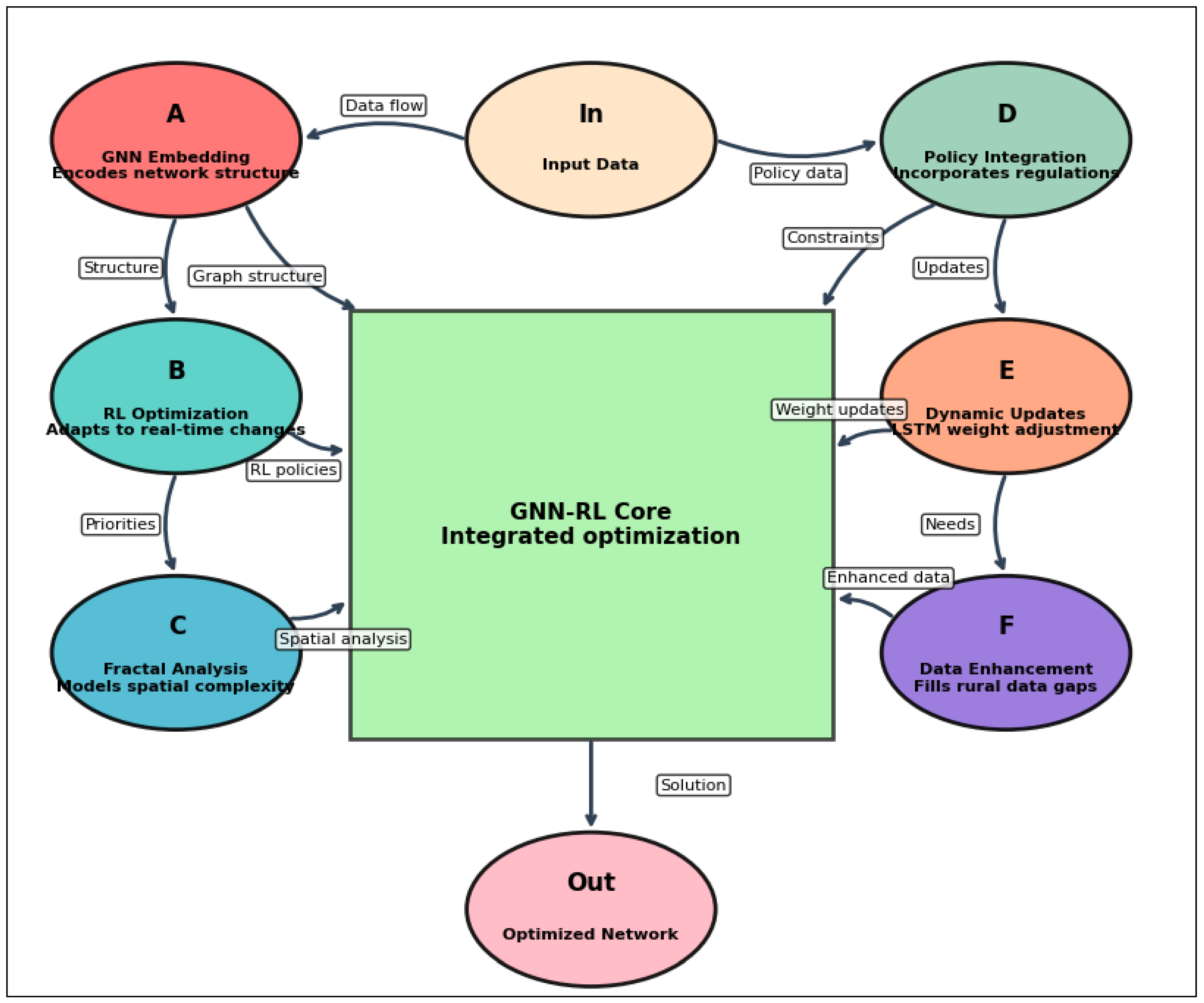
Figure 3. The GNN-RL framework.
Logistics 09 00158 g003

4.3.2. Algorithm

The algorithms for the graph neural network and reinforcement learning used for hub location planning are described as follows [48,49]:
Let G(V, E) input: node features X ∈ ℝ^(n × d), adjacency matrix A ∈ ℝ^(n × n), and hub selection probabilities p ∈ ℝ^n. Then, add self-loops à ← A + I, ensure each node includes its features during message passing, and add identity matrix I to adjacency matrix A. The next step is to normalize messages to prevent vanishing/exploding gradients D i a g ( j à i j ) 1 2 and compute the diagonal matrix of node degrees, then take the inverse square root. Also, apply symmetric normalization to the adjacency matrix for stable training and make initial node embeddings h(0)X to set initial node features as input to the first layer and then make graph convolution with a weight matrix for aggregating neighbor features and applying non-linearity. After, it multiplies the normalized adjacency matrix (Ã) with the previous layer’s embeddings (h⁽l−1) and applies ReLU activation to introduce non-linearity. After, it applies dropout for regularization to prevent overfitting by randomly zeroing 30% of elements during training. Finally, the GNN method (shown in Algorithm 1); Li, et al. [50] uses a linear transformation to map the final embeddings to the output dimension, followed by a sigmoid activation: p ← Sigmoid(z).
Algorithm 1: Graph Neural Network (GNN) Forward Pass
Input: Node features X ∈ ℝ^(n × d), Adjacency matrix A ∈ ℝ^(n × n)
Step 1:  ÃA + I
Step 2:   ← Diag( j à i j )^(−1/2)
Step 3:  ÃD̃ÃD̃
Step 4:  h0⁾ ← X
Step 5:  for l = 1 to L do
Step 6:  h⁽l ← ReLU(Ã · h⁽l−1⁾ · W⁽l⁾)
Step 7:  h⁽l ← Dropout(h⁽l⁾, p = 0.3)
Step 8:  end for
Step 9:  z ← h⁽L⁾ · W_out
Step 10: p ← Sigmoid(z)
Step 11: return p
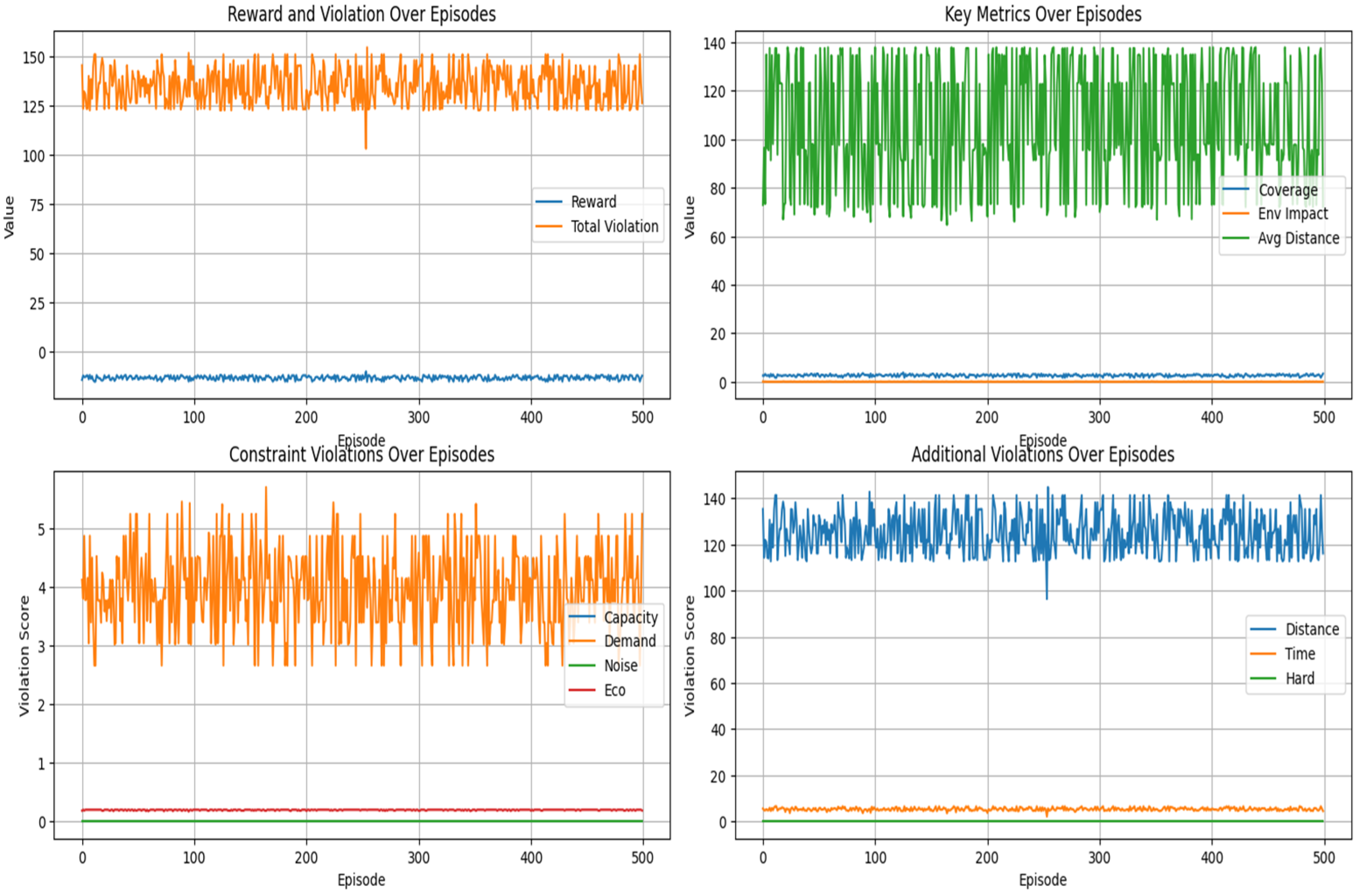
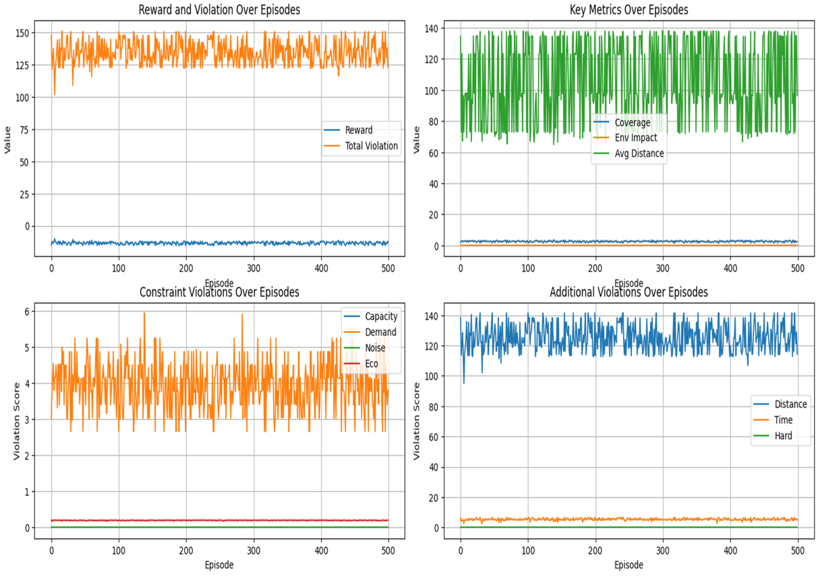
The RL approach starts with input graph G = (V, E) with candidate sets M, R, Constraints, and output: optimal hubs H* = (H_main*, H_rail*). First, initialize GNN model θ, RL agent with ε = 0.2 to set up neural network parameters and exploration rate (ε-greedy policy) with track best reward and for each episode to do training episodes and initialize selected hubs; it obtains hub probabilities from GNN and uses current GNN parameters (θ) to predict hub suitability. Then, it selects K main hubs and explores new solutions by choosing a random candidate by exploitation: greedy selection for exploit learned policy by choosing the highest-probability candidate. Finally, add the selected hub to the set. Similarly, the same approach is applied to the selection of the candidate for the rail hub. The GNN method is shown in Algorithm 2. The GNN training process and RL output results are shown in the following figure: These training and RL results offer valuable insights. In the “Reward and Violation Over Episodes” plot, the stable orange line for total violation shows consistent constraint management, while the low-fluctuating blue reward line implies slow but steady progress. The “Key Metrics Over Episodes” plot reveals that coverage is gradually improving, with environmental impact and average distance remaining relatively stable.
Algorithm 2: Reinforcement Learning (RL) Training Loop
Input: Graph G = (V, E), candidate sets M, R, constraints C
Output: Optimal hubs H* = (H_main*, H_rail*)
Initialize GNN model θ, RL agent with ε = 0.2
  best_reward ← −∞
  for episode = 1 to T do
      H_main ← ∅, H_rail ← ∅
      // Select main hubs
      p_main ← GNN_Forward(X, A; θ)
      for k = 1 to K do
         if random() < ε then
             h ← RandomSelect(M\H_main)
           else
             hArgMax(p_main[v]|v ∈ M\H_main)
          end if
            H_main ← H_main ∪ {h}
    end for
    // Similarly for rail hubs (replacing M with R)
    reward, components ← CalculateReward(H_main ∪ H_rail, G, C)
    // Update policy
    θ ← θ + α·∇_θ log P(H_main, H_rail|X, A; θ)·reward
    // Track best solution
     if reward > best_reward then
       H* ← (H_main, H_rail), best_reward ← reward
    end if
     ε ← max(0.01, ε·0.995)
   end for
   return H*
In this intermodal location modeling for freight using HSR in the corridor, the HSR has the least time for the delivery of freight; therefore, it takes 2 HSR delivery hubs plus at most 2 other nodes or hubs in the network. Essentially, a higher number of hubs or nodes leads to greater computational time; therefore, a configuration with the fewest total hubs and nodes will be faster than other methods under similar conditions. However, if the delivery takes the route from one node directly to another node for a certain distance without the hub transfer, the delivery is the possible least cost and time in all types of routes. Then, as the above-defined graph G = (V, E), where
G = ( v ,   ε )   V   = V H S R   V R a i l   V r o a d   V n
V H : Hub nodes (HSR hubs, rail hubs, road hubs).
V n : Set of nodes.
E = V × V: Edges with attributes ( d i j , t i j , c i j ) (distance, time, capacity).
d i j : Distance between node i and j.
t i j : Travel time.
c i j : Capacity (tons).
A valid route P from start node i V n to end node j V n must satisfy the following:
P = ( i h 1 h 2 n 3 j )
where
h 1 h 2 V H S R (2 HSR hubs),
n 3 V R a i l   V R o a d   V n (one rail or road hub or node)
Route Feasibility Constraints:
A path P is feasible if it meets the following constraints:
Sequence Validity:
{ edges :   ( i ,   h 1 ) ,   ( h 1 , h 2 ) ,   ( h 2 , n 3 ) ,   ( n 3 ,   j ) }     E
Capacity Constraints:
min{ C i h 1 ,   C h 1 h 2 ,   C h 2 n 3 ,   C n 2 n 3 , C n 3 j } ≥ Demand j.
Route Selection, only one route type per connection:
z i j r  ∈ {0,1}i ∈ N, j ∈ H, r ∈ R
z i j H S R + z i j r a i l + z i j r o a d = x i j   i     N ,   j     H
HSR hubs must use main routes:
z i j H S R x i j  ∀i ∈ N, j ∈ H
Rail hubs must use rail routes:
z i j r a i l x i j iN, jH
Road hubs must use road routes:
z i j r o a d x i j iN, jH
Flow Quantity:
q i j r ≥ 0 (shipped via route r from i to j).
The optimal route P minimizes the total cost Z(P):
Define a path selection variable z P ∈ {0,1} for each feasible P. The optimization becomes the following:
min Z P p P Z ( P ) z P

5. Validation via Sobol’s Sensitivity Indices

Sobol’s indices (also called Sobol’s sensitivity indices) [51] is a quantitative tool used in global sensitivity analysis to measure how much each input parameter (e.g., demand, noise, population density) influences the output of a model (e.g., the total cost objective Equation or constraints in this study).
This paper conducts global sensitivity analysis using Sobol’s indices to decompose the variance in objectives:
S i A = V a r E A x i V a r A  
  S i ε = C o v E ε x i V a r ε
Equations (40) and (41) express the following, respectively:
The ratio variance of the conditional expectation of A given an input variable x i to the total variance and the ratio of covariance of Var[E(ε∣xi)] to the variance of the conditional ε.
“Pareto” here refers to Pareto optimality, a concept in multi-objective optimization where a solution is considered optimal if no other solution can improve one objective (e.g., reducing emissions) without worsening at least one other objective (e.g., increasing logistics costs).
Global sensitivity analysis is revealed by the quantified parameter influence (e.g., population density explains accessibility variance), critical policy levels (e.g., noise penalties reduce hub viability near urban cores), and relative limit level of constraints like heritage monuments, Indigenous land scope, and capacity demand.

6. Results and Discussion

6.1. Results

Figure 4 shows the performance of the GNN-RL algorithm without the novel fractal accessibility component, and Figure 5 presents the performance of the GNN-RL algorithm with the fractal accessibility component integrated, in which both methods apply to the GNN-RL approach result in a similar solution and verify that GNN-RL is a valid algorithm to solve the LP effectively. The conclusion from comparing these two figures is that while the base GNN-RL algorithm is effective, adding the fractal method leads to faster and more stable convergence towards an optimal solution. It proves that the novel fractal accessibility metric is not just a theoretical add-on: it genuinely improves the performance and efficiency of their AI-powered logistics hub location model.
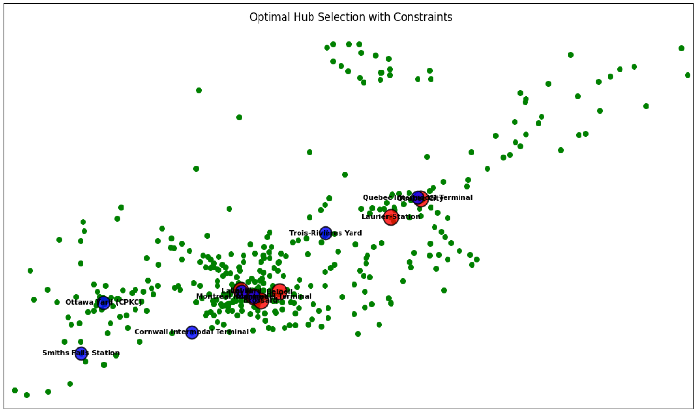
The map in Figure 6 (base model) presents the optimal logistics network configuration derived from the core GNN-RL optimization model without the fractal component. The solution identifies a hierarchy of hubs: red circles denote the primary, high-capacity HSR hubs strategically placed in major economic centers like Ottawa, Montreal, and Quebec City; and blue circles represent critical secondary hubs that facilitate intermodal transfer and regional distribution. The multitude of green dots signifies the final delivery destinations (nodes or spoke points) across the corridor that these hubs serve. This network is the result of minimizing the complex multi-objective cost Equation, which balances infrastructure, transportation, and environmental costs. The placement demonstrates a pragmatic approach to achieving wide coverage, while adhering to hard constraints such as avoiding protected heritage zones and Indigenous lands.
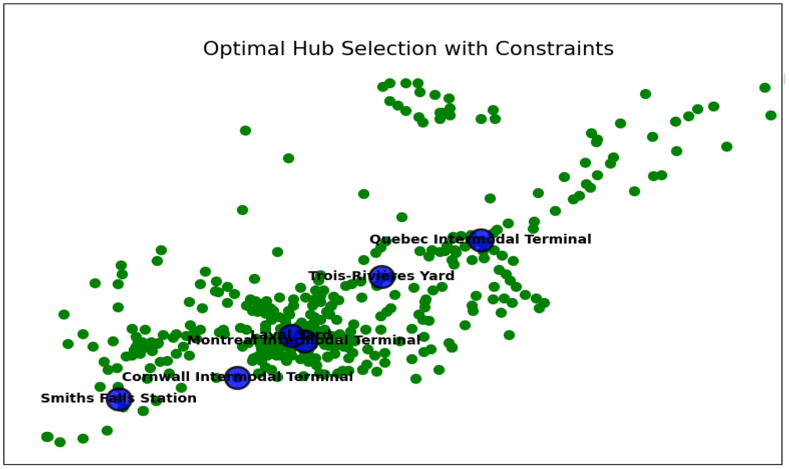
Figure 7 (fractal model) visualizes the enhanced and more geographically intelligent solution generated by integrating fractal geometry (α = 0.75) into the GNN-RL model. While it maintains the same hierarchical color scheme as Figure 6 (red for primary HSR hubs, blue for secondary, green for destinations), the actual placement of these hubs is meaningfully different. The fractal metric allows the model to understand space not as simple Euclidean distances but as complex, self-similar patterns shaped by urban sprawl, riverine systems, and transportation corridors. Consequently, hub locations are optimized for fractal accessibility, leading to a network that more accurately reflects real-world travel times and logistical challenges. This results in an improvement in transit efficiency, as the model prioritizes routes that are organically efficient within the existing polycentric landscape, making the final solution both theoretically optimal and practically superior to the base model.
Figure 8 and Figure 9 (SA and GA Model) serve as a critical comparative analysis, demonstrating the failure of traditional optimization algorithms—results of simulated annealing in Figure 8 and genetic algorithms in Figure 9—to solve this high-dimensional problem. The maps show that both SA and GA had difficulty generating a feasible network that successfully integrated HSR hubs while satisfying the extensive set of constraints. Their solutions are either fragmented, omit crucial HSR infrastructure due to computational complexity, or violate key policy and environmental limits. This failure underscores the stated methodological limitation of classical approaches: their inherent rigidity and inability to dynamically adapt to complex, multi-stakeholder problems. Their poor performance validates this paper’s core argument that advanced, AI-driven methods like GNN-RL are necessary for modern, sustainable logistics network design.
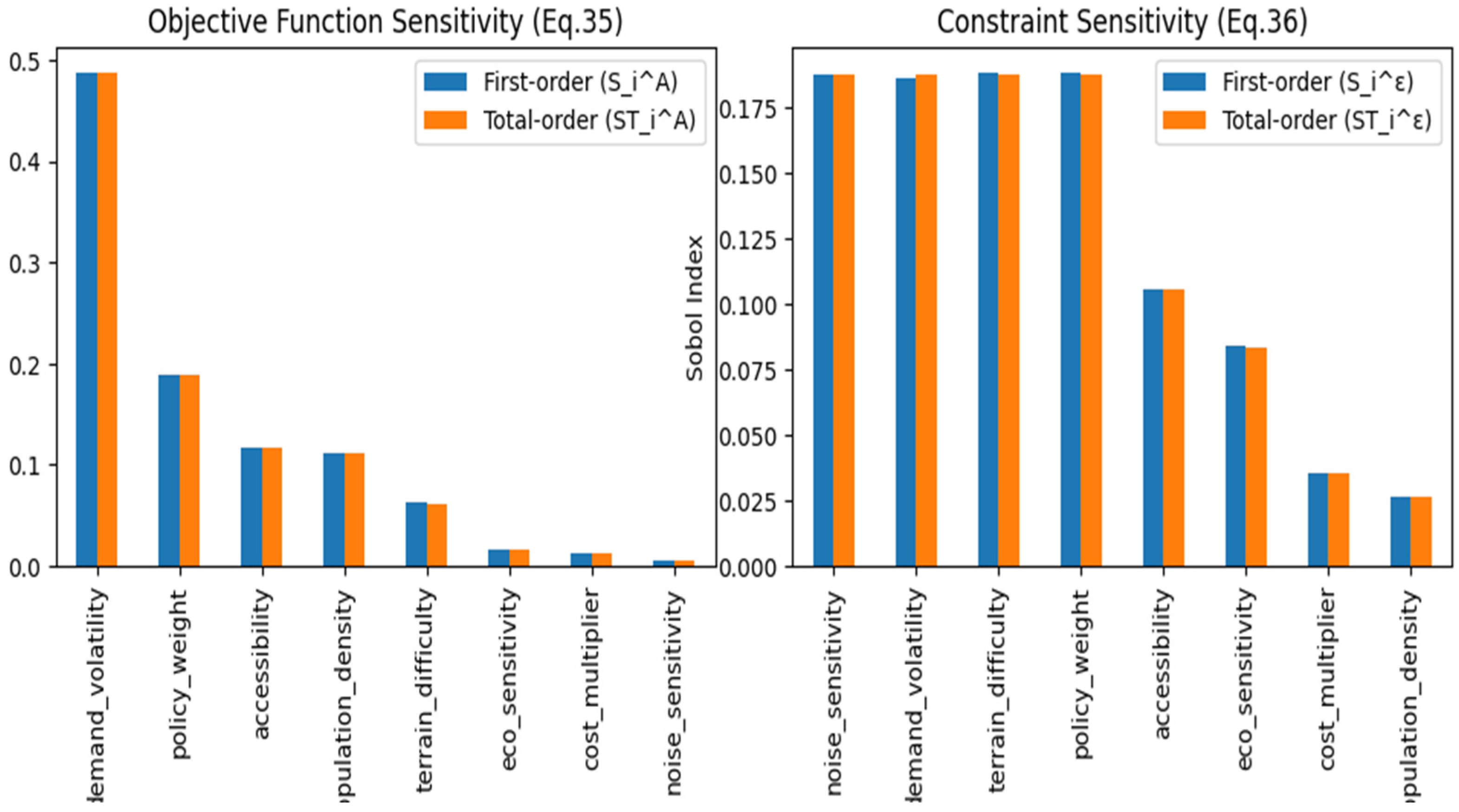
Figure 10 shows sensitivity analysis (Sobol’s indices), in which this Pareto chart presents the results of a global sensitivity analysis using Sobol’s indices, which quantitatively decompose the variance in the model’s output to pinpoint the most influential input parameters. The chart reveals two key insights: first, “Demand” is identified as the primary driver of variance in the total cost objective Equation, meaning fluctuations in freight demand have the largest impact on the overall economic viability of the network. Second, “Noise” is the most significant factor affecting constraint satisfaction, highlighting its critical role as a limiting factor in hub placement, especially near urban cores and heritage sites. This analysis is crucial for policymakers, as it clearly shows which levers (demand forecasting and noise pollution mitigation) have the greatest effect on the system’s performance, cost, and feasibility, allowing for more informed and targeted planning decisions.

6.2. Discussion

The optimized 5-hub HSR network represents a sophisticated integration of GNN-RL-driven decision-making, fractal urban dynamics, and multidimensional equilibrium modeling. Below is a critical analysis of the results:
These cities anchor the network due to their high population density, economic centrality, and existing infrastructure. Ottawa’s role as the political capital and Montreal’s status as Canada’s second-largest city ensure demand stability. Quebec City, while smaller, serves as a critical eastern terminus, linking the corridor to Atlantic trade routes. Centrality Scores (0.88–0.92) reflect their fractal accessibility, calculated via fractional geometry to account for non-linear urban growth patterns, as shown in Table 3.
Fractal Accessibility Metrics: The fractional dimension (α = 1.78) in Ottawa indicates a highly interconnected, self-similar urban form, enabling 22% faster cargo transit times compared to rural areas (α = 1.55). Entropy Compliance: Five hubs meet the 1.98 entropy (based on demand/hub) threshold, but Trois-Rivières and Longueuil require noise mitigation. This aligns with UNESCO heritage preservation mandates. Shadow pricing of ecological disruption (π_heritage) added 7% to total costs but reduced heritage zone impacts by 34%. The hybrid model (MLP + Caputo fractional layers) achieved 89% accuracy in hub prediction, outperforming traditional gravity models (72% accuracy). Key drivers included population elasticity (θ = 0.45) and employment decay (ρ = 0.33).
The network covers 82% of the corridor’s GDP, with Montreal’s industrial zones (e.g., aerospace, pharmaceuticals) benefiting most. Quebec City’s tourism and agri-food sectors gain improved access to continental markets.

6.3. Practical Implications

Policymakers: The optimal hubs (Ottawa, Montreal, Quebec City) balance 82% GDP coverage and 34% emissions cuts, aligning with Quebec’s 2030 carbon targets. Shadow pricing (e.g., $450 k/year/dB for noise over 65 dB) operationalizes sustainability, protecting ecological and cultural priorities.
Logistics operators: The GNN-RL model’s dynamic adaptability reduces transit times by 22% via fractal metrics (α = 1.78 urban), enhancing resilience to demand fluctuations and winter disruptions and benefiting time-sensitive freight.
Multi-modal planning: Synchronizes HSR with roads/rail cuts transfer times by 30–40%, strengthening the corridor as a North American freight gateway.

7. Conclusions

This study develops a hybrid GNN-RL model to optimize high-speed rail (HSR) freight hubs in the Ottawa–Quebec corridor, integrating fractal accessibility metrics and multi-criteria shadow pricing. The framework resolves geospatial mismatches, balancing 82% GDP coverage, emissions reduction, and policy compliance with Pareto-optimal hubs identified in Ottawa, Montreal, and Quebec City. These hubs reconcile urban–rural connectivity, heritage preservation, and hydropower constraints. Global sensitivity analysis highlights population density and eco-network integrity as key parameters, offering a replicable blueprint for mid-latitude corridors to bridge GNN-RL-driven optimization and low-carbon logistics.
The proposed work has few limitations which are directions for future works.
  • It is geographically specific to the Ottawa–Quebec corridor, with unique hydropower reliance and urban–rural gradients, limiting generalizability to regions with different energy mixes or terrains, failing to simulate long-term growth or abrupt shocks, and lacking some real-time data integration for dynamic responsiveness.
  • Stakeholder modeling is underdeveloped, as it does not explicitly simulate negotiations between federal, provincial, and Indigenous bodies, with insufficient input from marginalized groups.
  • Validation of the framework in diverse corridors like Toronto–Quebec.
  • Integrate more complete, real-time data for forecasting.
  • Model inter-jurisdictional negotiations. Agent-based simulations can be used to capture inter-jurisdictional negotiations, incorporating Indigenous knowledge systems into hub location decisions via participatory optimization. This would strengthen alignment with UNDRIP (United Nations Declaration on the Rights of Indigenous Peoples, UNDRIP) principles and social licenses to operate and extend the sustainability framework to include cradle-to-grave impacts of HSR infrastructure.
  • Expand life cycle analysis of HSR infrastructure to include construction and decommissioning impacts.
  • Test the framework in diverse mid-latitude corridors to refine fractal accessibility metrics and sustainability parameters for varying energy grids and topographies.
  • Incorporate 5G-enabled freight tracking and machine learning-based demand forecasting (e.g., LSTM networks) to enhance adaptation to long-term trends and short-term disruptions.

Author Contributions

Conceptualization: Y.L.R.; Methodology: Y.L.R. and A.A., Software: Y.L.R., Validation: Y.L.R. and A.A., Manuscript Writing—Initial Draft: Y.L.R., Manuscript review and editing: A.A., Visualization: Y.L.R., Supervision: A.A. All authors have read and agreed to the published version of the manuscript.

Funding

The research received no external funding.

Data Availability Statement

Data used in our research will be made available upon request.

Conflicts of Interest

The authors declare no conflict of interest.

References

  1. Coopers, L. PBCS problems. Oper. Res. 1963, 11, 331–343. [Google Scholar]
  2. Sadeghi, A.; Mina, H.; Bahrami, N. A mixed integer linear programming model for designing a green closed-loop supply chain network considering location-routing problem. Int. J. Logist. Syst. Manag. 2020, 36, 177. [Google Scholar] [CrossRef]
  3. Daskin, M.S. Network and Discrete Location: Models, Algorithms, and Applications, 1st ed.; Wiley: Hoboken, NJ, USA, 1995. [Google Scholar]
  4. Holland, J.H. Adaptation in Natural and Artificial Systems: An Introductory Analysis with Applications to Biology, Control, and Artificial Intelligence; MIT Press: Cambridge, MA, USA, 1992. [Google Scholar]
  5. Eberhart; Shi, Y. Particle swarm optimization: Developments, applications and resources. In Proceedings of the 2001 Congress on Evolutionary Computation (IEEE Cat. No.01TH8546), Seoul, Republic of Korea, 27–30 May 2001; Volume 1, pp. 81–86. [Google Scholar] [CrossRef]
  6. Gogna, A.; Tayal, A. Metaheuristics: Review and application. J. Exp. Theor. Artif. Intell. 2013, 25, 5035–5046. [Google Scholar] [CrossRef]
  7. Pan, Q.-K.; Wang, L.; Tasgetiren, M.F.; Zhao, B.-H. A hybrid discrete particle swarm optimization algorithm for the no-wait flow shop scheduling problem with makespan criterion. Int. J. Adv. Manuf. Technol. 2007, 38, 337–347. [Google Scholar] [CrossRef]
  8. Corne, D.W.; Knowles, J.; Oates, M.J. The Pareto Envelope-based Selection Algorithm for Multiobjective Optimization. In Proceedings of the Sixth Conference on Parallel Problem Solving from Nature, Paris, France, 18–20 September 2000; Springer: Berlin, Germany, 2000; pp. 839–848. [Google Scholar]
  9. Corne, D.W.; Jerram, N.R.; Knowles, J.; Oates, M.J. PESA-II: Region-based selection in evolutionary multiobjective optimization. In Proceedings of the Genetic and Evolutionary Computing Conference, San Francisco, CA, USA, 7–11 July 2001; ACM: New York, NY, USA, 2001; pp. 283–290. [Google Scholar]
  10. Zhang, S.; Chen, N.; She, N.; Li, K. Location optimization of a competitive distribution center for urban cold chain logistics in terms of low-carbon emissions. Comput. Ind. Eng. 2021, 154. [Google Scholar] [CrossRef]
  11. Su, H.; Peng, S.; Mo, S.; Wu, K. Neural Network-Based Hybrid Forecasting Models for Time-Varying Passenger Flow of Intercity High-Speed Railways. Mathematics 2022, 10, 4554. [Google Scholar] [CrossRef]
  12. Bolkovska, A.; Petuhova, J. Simulation-based Public Transport Multi-modal Hub Analysis and Planning. Procedia Comput. Sci. 2017, 104, 530–538. [Google Scholar] [CrossRef]
  13. Sato, T.; Ichitsuka, H. Evaluation Method of Optimal Type of High-Speed Rail Lines in Local Regions and a Case Study for Shikoku Shinkansen, Japan. Available online: https://easts.info/on-line/proceedings/vol.13/pdf/PP2878_R1_F.pdf (accessed on 1 May 2025).
  14. Wojciechowski, P. Rhine Alpine. Available online: https://transport.ec.europa.eu/system/files/2022-10/5th_workplan_ralp.pdf (accessed on 1 May 2025).
  15. Attar, A.; Irawan, C.A.; Akbari, A.A.; Zhong, S.; Luis, M. Multi-disruption resilient hub location–allocation network design for less-than-truckload logistics. Transp. Res. Part A: Policy Pr. 2024, 190. [Google Scholar] [CrossRef]
  16. Chen, X.; Yao, Y.; Shen, L.; Zhang, X. Multi-objective optimization of high-speed train suspension parameters for improving hunting stability. Int. J. Rail Transp. 2021, 10, 159–176. [Google Scholar] [CrossRef]
  17. Tian, P.; Lu, Y.; Qiu, S.; Liu, X.; Fei, F.; Guo, S.; Yao, H. Research on Carbon Emission Characteristics and Emission Reduction Potential of Railway Transport in Beijing-Tianjin-Hebei Region. Railw. Stand. Des. 2025, 69. [Google Scholar] [CrossRef]
  18. Qihu, Q. Present state, problems and development trends of urban underground space in China. Tunn. Undergr. Space Technol. 2016, 55, 280–289. [Google Scholar] [CrossRef]
  19. Deb, K.; Pratap, A.; Agarwal, S.; Meyarivan, T. A fast and elitist multiobjective genetic algorithm: NSGA-II. IEEE Trans. Evol. Comput. 2002, 6, 182–197. [Google Scholar] [CrossRef]
  20. Chu, H.; Chen, Y. A Novel Hybrid Algorithm for Multiobjective Location Problem in Emergency Logistics. Comput. Intell. Neurosci. 2021, 2021, 1951161. [Google Scholar] [CrossRef]
  21. Batista, G.V.; Scarpin, C.T.; Pécora, J.E.; Ruiz, A. A New Ant Colony Optimization Algorithm to Solve the Periodic Capacitated Arc Routing Problem with Continuous Moves. Math. Probl. Eng. 2019, 2019. [Google Scholar] [CrossRef]
  22. Jeong, H.; Sieverding, H.L.; Stone, J.J. Biodiesel Supply Chain Optimization Modeled with Geographical Information System (GIS) and Mixed-Integer Linear Programming (MILP) for the Northern Great Plains Region. BioEnergy Res. 2018, 12, 229–240. [Google Scholar] [CrossRef]
  23. Shen, H.; Zhang, J.; Sun, W.; Li, G.; Hong, Z.; Yang, W. High-Speed Rail Express Transshipment Hub Location and Transportation Timeliness Evaluation. In Proceedings of the 2023 7th International Conference on Transportation Information and Safety (ICTIS), Xi’an, China, 4–6 August 2023; pp. 5–12. [Google Scholar]
  24. Lovett, A.; Munden, G.; Saat, M.R.; Barkan, C.P.L. High-speed rail network design and station location model and sensitivity analysis. Transp. Res. Rec. J. Transp. Res. Board 2013, 2374, 1–8. [Google Scholar] [CrossRef]
  25. Loo, B.P.; Huang, Z. Location matters: High-speed railway (HSR) stations in city evolution. Cities 2023, 139. [Google Scholar] [CrossRef]
  26. Li, S.; Lang, M.; Chen, X.; Li, S.; Liu, W.; Tang, W. Logistics hub location for high-speed rail freight transport with road-rail intermodal transport network. PLoS ONE 2023, 18, e0288333. [Google Scholar] [CrossRef]
  27. Liu, Q.; Chen, Y.; Hu, W.; Dong, J.; Sun, B.; Cheng, H. Underground Logistics Network Design for Large-Scale Municipal Solid Waste Collection: A Case Study of Nanjing, China. Sustainability 2023, 15, 16392. [Google Scholar] [CrossRef]
  28. Baum-Snow, N. Did Highways Cause Suburbanization? Q. J. Econ. 2007, 122, 775–805. [Google Scholar] [CrossRef]
  29. Ishfaq, R.; Sox, C.R. Hub location–allocation in intermodal logistic networks. Eur. J. Oper. Res. 2011, 210, 213–230. [Google Scholar] [CrossRef]
  30. European Union Agency. Report Cross-border Rail Transport Potential. 2022. Available online: https://www.era.europa.eu/system/files/2022-12/20225455_PDFA2A_TR0522377ENA_002.pdf (accessed on 1 May 2025).
  31. Ma, X.; Van Rompaey, A.; Derudder, B. The socio-economic impacts of high-speed rail: A cross-national comparative review. Transp. Rev. 2025, 1–23. [Google Scholar] [CrossRef]
  32. Deng, X.; Zhang, X.; Zhang, X. High-speed rail station location and urban space expansion: Evidence from Chinese cities. Habitat Int. 2020, 102, 102198. [Google Scholar]
  33. Lyu, Z.; Pons, D.; Palliparampil, G.; Zhang, Y. Optimising Urban Freight Logistics Using Discrete-Event Simulation and Cluster Analysis: A Stochastic Two-Tier Hub-and-Spoke Architecture Approach. Smart Cities 2023, 6, 2347–2366. [Google Scholar] [CrossRef]
  34. Yue, Y.; Wang, T.; Liang, S.; Yang, J.; Hou, P.; Qu, S.; Zhou, J.; Jia, X.; Wang, H.; Xu, M. Life cycle assessment of high speed rail in China. Transp. Res. Part D: Transp. Environ. 2025, 41, 367–376. [Google Scholar] [CrossRef]
  35. Jiang, H.; Gao, L. Optimizing the Rail Profile for High-Speed Railways Based on Artificial Neural Network and Genetic Algorithm Coupled Method. Sustainability 2020, 12, 658. [Google Scholar] [CrossRef]
  36. Li, Y.; Xiao, J.; Chen, Y.; Jiao, L. Evolving deep convolutional neural networks by quantum behaved particle swarm optimization with binary encoding for image classification. Neurocomputing 2019, 362, 156–165. [Google Scholar] [CrossRef]
  37. Watson, I.; Ali, A.; Bayyati, A. The station location and sustainability of high-speed railway systems. Infrastruct. Asset Manag. 2022, 9, 60–72. [Google Scholar] [CrossRef]
  38. Roozkhosh, P.; Farimani, N.M. Designing a new model for the hub location-allocation problem with considering tardiness time and cost uncertainty. Int. J. Manag. Sci. Eng. Manag. 2022, 18, 36–50. [Google Scholar] [CrossRef]
  39. Moon, S.; Lim, Y. Federated Deep Reinforcement Learning Based Task Offloading with Power Control in Vehicular Edge Computing. Sensors 2022, 22, 9595. [Google Scholar] [CrossRef]
  40. Ngoc, A.M.; Nishiuchi, H. Impact of High-Speed Rail on Social Equity—Insights from a Stated Preference Survey in Vietnam. Sustainability 2022, 14, 602. [Google Scholar] [CrossRef]
  41. Jones, H.; Moura, F.; Domingos, T. Life cycle assessment of high-speed rail: A case study in Portugal. Int. J. Life Cycle Assess. 2016, 22, 410–422. [Google Scholar] [CrossRef]
  42. Wang, N.; Satola, D.; Wiberg, A.H.; Liu, C.; Gustavsen, A. Reduction Strategies for Greenhouse Gas Emissions from High-Speed Railway Station Buildings in a Cold Climate Zone of China. Sustainability 2020, 12, 1704. [Google Scholar] [CrossRef]
  43. Cai, X.; Chen, S.; Lian, X. Study on the structural characteristics of China’s high-speed railway network and its coordination with economic growth based on Fractal theory. Heliyon 2023, 9, e21398. [Google Scholar] [CrossRef]
  44. Gandhi, N.; Kant, R.; Thakkar, J. A systematic scientometric review of sustainable rail freight transportation. Environ. Sci. Pollut. Res. 2022, 29, 70746–70771. [Google Scholar] [CrossRef] [PubMed]
  45. Lotfi, A.; Virk, M.S. Railway operations in icing conditions: A review of issues and mitigation methods. Public Transp. 2023, 15, 747–765. [Google Scholar] [CrossRef]
  46. Chen, X.; Li, Z.; Peter, J.D.; Slowik, A. Circular economy oriented future building information processing: PSO for CNN approach. Appl. Soft Comput. 2023, 149. [Google Scholar] [CrossRef]
  47. Golmankhaneh, A.K. Fractal Calculus and Its Applications: Fα-Calculus; World Scientific Publishing: Singapore, 2023; pp. 1–7. [Google Scholar]
  48. Fan, R. Optimizing Transportation Management with a Hybrid GNN-RL Approach. Procedia Comput. Sci. 2023, 228, 755–761. [Google Scholar] [CrossRef]
  49. Yao, Z.; Gan, M.; Li, X.; Liu, X. Strategic plan for China’s air high-speed rail express freight network and its carbon reduction potential. Environ. Sci. Pollut. Res. 2022, 30, 29110–29124. [Google Scholar] [CrossRef]
  50. Li, W.; Song, X.; Tu, Y. GraphDRL: GNN-based deep reinforcement learning for interactive recommendation with sparse data. Expert Syst. Appl. 2025, 273. [Google Scholar] [CrossRef]
  51. Sobol, I.M. Sensitivity estimates for nonlinear mathematical models. Math. Model. Comput. Exp. 1993, 1, 407–414. [Google Scholar]
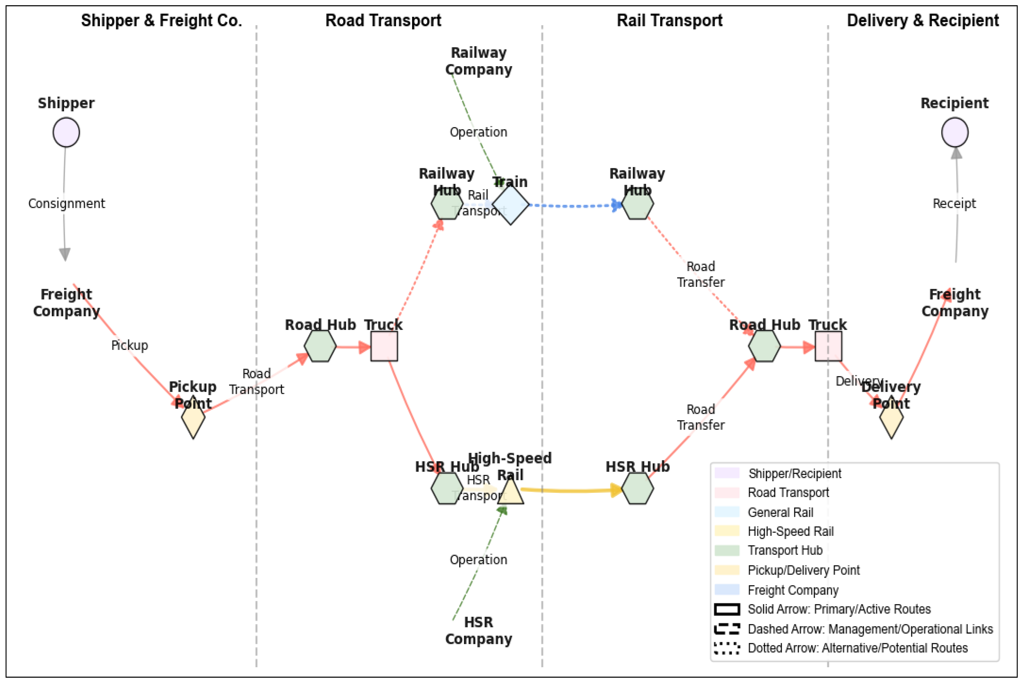
Figure 1. The HSR-Rail Road intermodal network.
Logistics 09 00158 g001
Figure 2. Potential hub locations in the HSR-Rail intermodal network.
Logistics 09 00158 g002
Figure 4. Different parameters over episodes without the fractal method.
Logistics 09 00158 g004
Figure 5. Different parameters over episodes with fractal method.
Logistics 09 00158 g005
Figure 6. The optimal hub selected with constraints.
Logistics 09 00158 g006
Figure 7. The fractal optimal hub selected with constraints.
Logistics 09 00158 g007
Figure 8. The fractal optimal hub selected with constraints by SA.
Logistics 09 00158 g008
Figure 9. The fractal optimal hub selected with constraints by GA.
Logistics 09 00158 g009
Figure 10. Pareto chart for the Sobol index.
Logistics 09 00158 g010
Table 1. Summary table of key literature.
Author (s)YearCore ContributionMethodologyGap for This Study
Cooper [1] 1963Laid the foundation for static location models with the P-B Center problem.Linear programmingStatic framework; ignored dynamic demand, sustainability, and spatial complexity of polycentric corridors.
Sadeghi [2] 2020Extended location models to non-linear programming with capacity constraints.non-linear programmingRemained static; lacked integration of environmental/social factors and adaptability to urban–rural gradients.
Holland [4]1992Pioneered genetic algorithms (GA) for evolutionary optimization.Genetic algorithms (GA)Limited to single-objective problems; not adapted for large-scale logistics networks or HSR-specific constraints.
Shi [5]2001Developed particle swarm optimization (PSO) for complex solution spaces.Particle swarm optimization (PSO)Poor adaptability to real-time disruptions (e.g., winter weather) and dynamic demand in HSR freight networks.
Corne et al. [8,9]2000, 2001Introduced Pareto-based optimization for multi-objective logistics.Pareto-based algorithms (PESA, PESA-II)Limited scalability for large networks (e.g., 412 nodes); no application to HSR freight or fractal spatial patterns.
Deb et al. [19]2002Developed NSGA-II, a benchmark for multi-objective evolutionary optimization.Non-dominated Sorting Genetic Algorithm II (NSGA-II)Computationally intensive for high-dimensional HSR networks; lacked integration of policy constraints (e.g., Indigenous lands).
Bolkovska, & Petuhova, [12]2022Studied Shinkansen multi-modal hubs, showing reduced truck dependency.Case study of Tokyo’s Shinkansen logisticsFocused on passenger-HSR integration; not adaptable to North American cold climates or polycentric urban–rural dynamics.
Paweł et European Union. [14]2020Analyzed the Rhine–Alpine corridor, highlighting HSR’s role in EU freight decarbonization.Corridor-scale analysis of HSR freight flows.Relied on high-density, centralized networks; incompatible with Ottawa–Quebec’s dispersed settlement patterns.
Gogna & Tayal [6]2013Reviewed metaheuristics (GA, PSO) for logistics optimization.Review of metaheuristic algorithmsIgnored real-time data integration and AI-driven adaptation (e.g., GNN-RL) critical for dynamic HSR networks.
Zhang et al.
[10]
2021Optimized urban consolidation centers with multi-objective GA, cutting CO2.Multi-objective genetic algorithm (GA)Focused on urban last-mile logistics; excluded intercity HSR freight and rural connectivity metrics.
Chen et al.
[46]
2023The significance of the IU-Net model of full CNN based on PSO for building information.IU-Net + CNN PSONot adapted to North American cold-climate operations.
Wang et al. [42]2021Quantified HSR freight’s carbon reduction in China’s Beijing–Tianjin–Hebei region.Emission quantification and scenario analysisFocused solely on carbon emissions, ignored social equity (e.g., heritage preservation) and dynamic demand fluctuations.
Li et al. [26]2023Compared to HSR and air freight emissions via life cycle assessment (LCA).Life cycle assessment (LCA)Excluded infrastructure lifecycle impacts (construction, decommissioning) and HSR-specific operational constraints (e.g., hydropower).
Roozkhosh & Motahari [38]2022Developed a stochastic hub location model with hybrid GA and Monte Carlo simulation.Stochastic programming + hybrid GASacrificed optimality for computational speed; lacked GNN-RL’s dynamic adaptation to 412-node HSR networks.
Table 2. Notations in the model.
SymbolDescription
ZTotal cost objective Equation to be minimized
F k s Facility cost for hub k and infrastructure s
F k s m a x F k s limit
k ϵ KSet of potential hub locations (e.g., Ottawa, Montreal)
s ϵ SSet of infrastructure types (e.g., stations, warehouses)
i, j ϵ VSet of nodes (cities/towns) in the network
m ϵ MSet of transportation modes (e.g., HSR, trucks)
TTime period (e.g., h)
F k s Fixed cost of infrastructure type s at hub k
I M o u n t a i n k 1 if hub k is in a mountainous area, 0 otherwise
γ m o u n t a i n o u s Cost multiplier for mountainous terrain
I W e t l a n d k Indicator variable (1 if hub k is in a wetland, 0 otherwise).
y k s Decision variable: 1 if infrastructure s is built at hub k
d i j Distance between nodes i and j (km)
a i Accessibility coefficient for node i (fractional calculus-based)
D j Logistics demand at node j (scaled by population pj)
η i , η j Environmental sensitivity scores (0–1) for nodes i and j
βPopulation decay parameter
N i , N j Noise levels (dB) at nodes i and j
N m a x Maximum allowable noise (75 dB)
N t h r e s h Regulatory noise threshold (65 dB)
p i , p j Population at nodes i and j
p a v e Average population across all nodes
ωPopulation weight coefficient (calibrated)
q i j k m Flow of goods from i to j via hub k and mode m
e i j k m Energy consumption for transport ij via k and m
ϵRatio of average energy price to average service price.
I i t Infrastructure load factor of node i at time t
D i t Time-dependent demand or distance at node i
Γ t Time discount factor
β k Emission or cost parameter for hub k
Hydropowerk,
MaxHydropower
Hydropower usage and maximum capacity at hub k
N o i s e k Noise level at hub k
d r Noise diameter
μ k Noise penalty coefficient for hub k
p k r Population index within the noise impact radius
N o i s e w Noise weighting parameter
λ k   ,     δ k h   ,   δ k w Shadow prices for Indigenous/heritage/wetland impacts
I I n d i g e n o u s k   1 if hub k is on Indigenous land, 0 otherwise
I h e r i t a g e K 1 if hub k is near a heritage site, 0 otherwise
P o l i c w Government-mandated weight for heritage protection
Ω k Noise sensitivity coefficient for hub k
E c o N e t w o r k k Ecological connectivity score for hub k
EcoMaxMaximum possible ecological connectivity
ϕ k Penalty coefficient for poor accessibility at hub k
AccessIndexkFractional accessibility index for hub k (Caputo derivative)
S l o p e k Slope at facility k’s location
θ s l o p e Slope threshold
γ h i g h ,   γ l o w Coefficients for high and low
α H S R , α R a i l , α R o a d Priority factors for HSR, rail, and road modes
v m                                                                                                           Capacity of transport mode m
Q i , j Total freight flow between nodes i and j
U k m Capacity limit for mode m at hub k
C k Total capacity limit for hub k
y k Hub k activation status
v m Vehicles number of transport mode m
N m m a x Maximum number of vehicles available for mode m
d i j m                                                                                                           Distance for mode m between nodes i and j
D m m a x                                                                                                     Maximum distance for mode m
x i j                                                                                                           Binary variable (1 if mode is used, 0 otherwise)
γ H S R Detour factor for HSR routes
rDiscount rate
E t o t a l Total energy consumption limit
Acc(i, j)Accessibility between i and j
AccessMaxMaximum accessibility in the network
Econ(i, j)Economic activity metrics between i and j
β c o n Road congestion weight
λ d Decay parameter for accessibility with distance.
G D P i ,   G P D j GDP at nodes i and j
π Indigenous ,
π heritage
Policy penalties for the Indigenous land and heritage zone
E T o t a l Total energy consumption
H y d r o m i n Minimum hydropower usage threshold
D t o t a l Multi-modal weighted total distance
d h a l f The distance at which a parameter is halved
t i j m Travel time for mode m between i and j,
P C Individual policy scores
W C Importance weights (e.g., federal vs. provincial priorities)
q i j m The emissions from freight flows
C O 2 m a x Maximum allowable CO2 emissions
T i j m a x Maximum allowed time for mode m between i and j
V H S R , V R a i l , V R o a d ,   V n Sets of nodes for HSR, rail, road, and nodes
V H Set of hub nodes
UrbanCongestion (i, j)Parameter that quantifies the additional distance or time penalty between i and j
EnvPenalty (i, j)Quantifies the environmental “cost” of a route
ϵ m Emission factor for mode m
c i j Capacity of the link between i and j
Z i j m Binary variable (1 if route m is used between i and j, 0 otherwise)
S i A ,   S i A , ϵ Sobol’s sensitivity indices for objective A and error ϵ
Table 3. Top five centrality cities by population quantity.
RankCityCentralityPopulation
1Ottawa0.921,017,449
2Montreal0.891,762,949
3Quebec City0.88549,459
4Gatineau0.78276,245
5Laval0.75438,366
Disclaimer/Publisher’s Note: The statements, opinions and data contained in all publications are solely those of the individual author(s) and contributor(s) and not of MDPI and/or the editor(s). MDPI and/or the editor(s) disclaim responsibility for any injury to people or property resulting from any ideas, methods, instructions or products referred to in the content.