Abstract
The reliability of the “last mile” of cold-chain logistics is crucial for food safety. This study investigated the effect of different packaging treatments on the quality of anhydrously preserved live Ruditapes philippinarum (R. philippinarum) in “last mile” cold chain disruption. The temperature profiles of three packaging treatments at ambient temperature (25 °C) were monitored. Quality assessment was conducted based on sensory scoring, survival rate, total viable count (TVC), water-holding capacity (WHC), pH, total volatile basic nitrogen (TVB-N), thiobarbituric acid-reactive substances (TBA), color, and texture. Low-frequency nuclear magnetic resonance (LF-NMR) and magnetic resonance imaging (MRI) were utilized to characterize the water state profile. The findings demonstrated a progressive increase in internal package temperature throughout the “last mile”, with packages containing additional ice packs more effectively maintaining lower temperature and restricting the migration of “hot spots” towards the center. Specifically, the package with three ice packs maintained a markedly lower temperature, which effectively inhibited microbial activity, lipid oxidation, and the production of alkaline substances, resulting in higher survival rates, water-holding capacity, texture, sensory acceptability, and immobilized water fraction. Furthermore, LF-NMR relaxation parameters showed strong correlations with various physicochemical indices, suggesting a potential approach for real-time quality monitoring. This study provides insights for maintaining live R. philippinarum quality during the “last mile”.
1. Introduction
The consumption of shellfish has increased over time, accounting for 26% of aquatic animal food consumption in 2021 [1]. China boasts abundant live aquatic resources, yielding a total of 68.659 million tons in 2022, with live shellfish accounting for 23.86% of the total output [2]. Live shellfish have gained popularity due to their delicious taste [3] and rich nutritional value [4]. However, such products are highly perishable, geographically specific, and seasonal and have a short shelf life. The transportation of live shellfish products poses challenges in maintaining their survival rates and freshness. Furthermore, with the growing trend towards omni-channel retailing, e-commerce has become increasingly common for the sale of live aquatic products. This shift underscores the need for effective and scientifically grounded preservation and delivery methods for live shellfish.
Previous studies [5,6] have demonstrated that anhydrous preservation is a more cost-effective technique for live shellfish compared to water preservation, resulting in lower mortality rates and reduced nutrient loss [7]. It remains critical to maintain low temperatures during the delivery process, from producers to consumers, to preserve the freshness and quality of the shellfish [8]. For example, Bi et al. [9] found that anhydrous delivery at low temperature (4 °C) effectively maintains the high quality and physiological conditions of clams. Similarly, Jiang et al. [10] found that live Patinopecten yessoensis can be preserved for up to 5 days on ice. Thus, the cold chain logistics system plays a vital role in ensuring the quality and longevity of live shellfish products during distribution.
Currently, domestic delivery of live seafood during business-to-business (B2B) operations primarily relies on conventional refrigerated trucks [11]. This process has garnered significant attention, with numerous studies [12,13,14] focusing on improving refrigeration equipment and delivery technologies. However, in the business-to-consumer (B2C) process, frequent “cold chain breakage” occur due to the absence of professional transport equipment. Typically, only insulated containers and ice packs are used to maintain the cold chain. This challenge during the final stage of the delivery process, often referred to as the “last mile” phenomenon, is marked by temperature fluctuations caused by uncertainties in delivery time, delayed receipt, and a lack of cold storage facilities [15]. The distribution of temperature within the container is also influenced by the number and placement of ice packs. Such fluctuation is known to accelerate deterioration of live shellfish quality. For instance, Teng et al. [16] found that repeated freeze–thaw cycles significantly reduced the protein content, fat content, malondialdehyde (MDA) levels, sulfhydryl (-SH) levels, and Ca2+-ATPase activity in live pacific oysters. Therefore, maintaining a stable, low temperature field is vital for preserving the quality and freshness of the stored shellfish during “last mile” delivery [17,18]. In addition to traditional quality change investigation, analysis of temperature distribution is helpful for identifying the optimal placement and quantity of ice packs needed to maintain a stable, low temperature field. Although COMSOL Multiphysics® has been successfully employed as the thermal modeling software package to study the “last mile” distribution method [19] based on temperature considerations, few studies have simulated the temperature field in the “last mile” for determining suitable packaging.
There has been no systematic study on the effects of temperature fluctuation during the “last mile” of the cold chain on live R. philippinarum. Therefore, this study aims to investigate quality changes in anhydrous-preserved live R. philippinarum during express delivery in the “last mile” of the cold chain. The live clams were preserved using different express packaging treatments. Firstly, COMSOL Multiphysics® was used to simulate the temperature field in the box. Then, quality assessment was conducted based on sensory scoring, survival rate, TVC, and various physicochemical parameters, including WHC, pH, TVB-N, and TBA. Additionally, color analysis, texture profile, LF-NMR, and MRI were employed for further evaluation of quality alterations in live R. philippinarum. This study provides a reference for optimizing logistics distribution conditions and improving the quality of live R. philippinarum.
2. Materials and Methods
2.1. Materials and Reagents
Thiobarbituric acid, trichloroacetic acid, sodium chloride, boric acid, 1,1,2,3-tetraethoxypropane, and hydrochloric acid was purchased from Sinopharm Chemical Reagent Co., Ltd. (Shanghai, China). All materials were of at least analytical purity.
2.2. Sample Preparation
Live Ruditapes philippinarum (R. philippinarum) specimens (shell length: 40 mm, thickness: 5 mm) were purchased from the Oriental International Aquatic Center in Shanghai. After being placed in an ice container, they were transported to the laboratory within 1 h and stored at 4 °C. Live specimens with good activity, similar size, and other characteristics were selected from the same batch as the experimental samples. To simulate potential cold chain disruptions during business-to-consumer (B2C) transactions, four experimental groups were established. The samples were randomly assigned to four groups, each weighing 1000 g. Every 250 g portion was packaged in sterile polyethylene (PE) food-safe plastic bags.
One group was kept at 4 °C in a refrigerator as a control (CK), while the remaining three groups were each placed in an aluminum foil insulation bag with one, two, or three ice packs (dimensions: 150 × 105 × 2.5 mm). These insulated bags were then transferred to foam boxes (outer dimensions: 340 × 220 × 165 mm, internal dimensions: 300 × 180 × 145 mm) with foam lids (dimensions: 340 × 220 × 22 mm). The walls, lid, and base of the foam boxes all had the same thickness of 22 mm. The groups were labeled as R-1, R-2, and R-3 according to the number of ice packs used. The quality of the sample was assessed at four time points (0 h, 12 h, 24 h, and 48 h) at ambient temperature (25 °C).
2.3. Temperature Measurement
To monitor temperature changes during storage, a copper–constantan thermocouple probe (KEYSIGHT 34970, Keysight Technologies, Santa Rosa, CA, USA) was calibrated with an ice–water mixture prior to use. The probe was connected to a portable data logger and placed at the center of the clam shells. This method followed the protocol described by Manzocco et al. [20]. Monitoring continued until the samples were deemed inedible.
2.4. Modeling
2.4.1. Physical Model
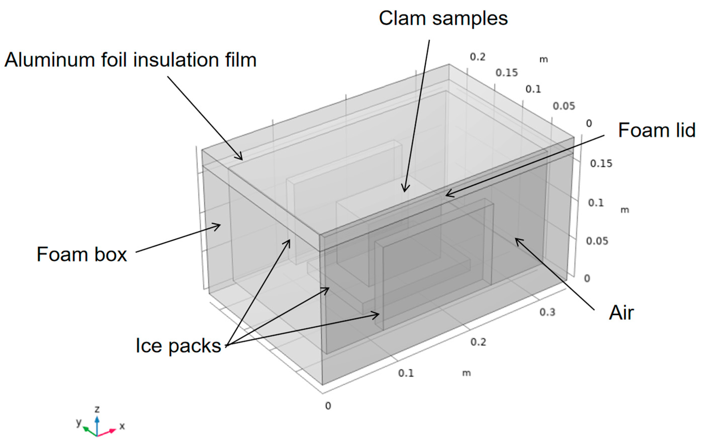
Figure 1 presents the physical geometry of the foam box. The outer dimensions of the box were 340 mm (length) × 220 mm (width) × 165 mm (height), while the internal dimensions were 300 mm (L) × 180 mm (W) × 145 mm (H). The thermostat requires insulation, such as foam, to separate the contents from the outside environment. To reduce heat transfer, aluminum foil insulation was then added to form a composite insulation layer with foam. This was followed by the addition of a source of cold, such as ice packs at −5 °C, which were placed vertically around the contents (clams). The remaining space in the interior was filled with air. The initial temperature of the contents was 5 °C.
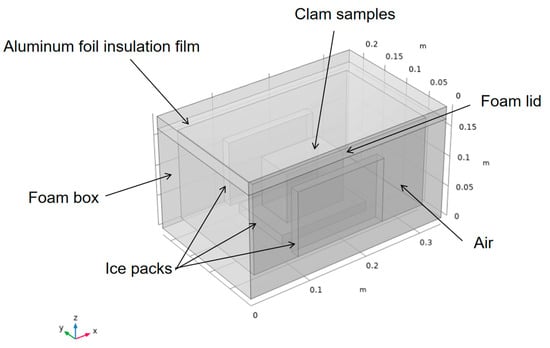
Figure 1.
Physical geometry of the box.
2.4.2. Assumptions and Governing Equation
To simplify the modelling process, the following assumptions were made:
- (1)
- All materials are considered isotropic.
- (2)
- The air inside the foam box is regarded as an incompressible fluid.
- (3)
- The initial temperature of the ice packs and the box interior is assumed to be uniform.
- (4)
- Changes in the density of the ice packs are neglected, thus assuming a constant volume for the ice packs [21].
The primary modes of heat transfer in the foam box include natural convection of the air inside the box and heat conduction between the internal components. In the context of cold food storage, the latent heat of phase change in the ice packs should also be considered.
The heat transfer within the solid and liquid phases follows the energy balance Equations (1) and (2):
The model fluid heat transfer Equations (3) and (4) are as follows:
where , , T, u, q, Q, , and are the density, specific heat capacity, temperature, external field dependent variable, heat flux, heat flow generated internally, internal energy, and kinetic energy, respectively. Because of the small effect of natural convection and the incompressible nature of air, and are negligible.
In addition, phase transition heat transfer is also involved. The phase change heat transfer Equations (5)–(9) are as follows:
where the subscript symbols phase1 and phase2 are liquid water and solid water (ice), respectively. , , , and are a percentage, the density, the specific heat capacity at constant pressure, and the thermal conductivity, respectively. The parameters for the phase change material (ice packs) used in the model, as provided by Perrot [22], are given in Table 1. The samples placed in the box are clams. Table 2 presents the characteristics of the clams.

Table 1.
Parameters of the phase change material (ice packs) used in the model.
Table 2.
Characteristics of the clams.
2.4.3. Initial Conditions and Boundary Conditions
The box walls consisted of insulation materials, and the ice packs were in direct contact with the internal surfaces of the box. The air temperature outside the box was constant, at 25 °C. The heat transfer boundary condition between the box surface and the air was set as natural convection with a convection heat transfer coefficient of 5 W·m−2·K−1, which was calculated using the following Equation (10):
where Q is the amount of heat exchanged between the clams and the atmosphere per unit time (W); h is the convective heat transfer coefficient (W·m−2·K−1); A is the surface area of the boundary between the food and the atmosphere (m2); T is the temperature of the food surface (°C), and T0 is the ambient temperature (°C). The box enclosure was set as thermal insulation.
The heat is transferred through the wall to the product at the bottom and then through the height of the product to the ice, causing it to melt and thereby inducing a phase change [24]. Under the relevant assumptions, the phase change heat transfer problem of water melting is simplified to a transient heat transfer problem, which only involves the first kind and third kind of boundary conditions.
2.4.4. Geometric Model Meshing and Numerical Solution
The box was nearly cuboid; thus, this shape was considered to simulate the geometric model of the box. A finite element method was employed to solve the transient heat transfer problem, enabling the calculation of temperature–time histories within the three-dimensional box model. The numerical solution was obtained using COMSOL Multiphysics Software 6.2. The model mesh was divided before model computing. A physics-controlled mesh consisting of tetrahedral area elements was generated for the simulations. For phase change materials, “finer” meshes must be used to accurately simulate the melting front. To reduce the amount of computer calculation and shorten the calculation time, other domains were set as “fine” tetrahedral meshes. The final grid system consisted of 57,481 domain elements (tetrahedral), 10,390 boundary elements (triangular), 916 edge elements (linear), and 60 vertex elements. The heat transfer inside the box varies with time, which requires instantaneous solving. In addition, the total time of the solution, initial time step, and relative tolerance were 48 h, 1 h, and 0.001, respectively. The server configuration for computing was a Lenovo processor, 13th Gen Intel (R) Core (TM) i9-13900HX, 2200 Mhz, 32 GB RAM, and a Win11 Server Standard 64-bit operating system.
2.4.5. Verification of Heat Transfer Model
Numerical and experimental results were compared to evaluate the accuracy of the model. One measure of forecast consistency, i.e., the root mean squared error (RMSE), was used to assess the reliability and accuracy of the heat transfer model [25], which can be calculated using the following Equation (11):
where Qi and Pi are the values of observed and predicted temperatures (°C); n is the number of observations; and Qi is the average of observed values. Values of RMSE close to 0 are considered to indicate better model prediction.
2.5. Sensory Evaluation
Sensory evaluations were conducted according to the method of Manousaridis et al. [26], with slight modifications. The sensory panel consisted of eight trained members. The results were recorded using a 10-point scale across four categories: color (0: dull, 10: milky white), smell (0: spoilage odor, 10: no off-odor), appearance (0: flesh detachment, 10: intact), and texture (0: high viscosity, 10: firm). The scores from these categories were averaged to calculate the overall “sensory score” (ranging from 0 to 10), and the acceptability was determined as having a score of over 6. Data were compiled from the independent evaluations of the eight panel members and presented as the mean score.
2.6. Survival Rate Assessment
Survival rate was measured according to the method of Gonçalves et al. [27], where the survival of clams was determined by observing their valve responses. Clams with open shells were gently tapped with a glass rod to monitor their reactions. The clam was considered dead if its shell remained open for an extended period. The survival rate was calculated using Equation (12):
Survival rate (%) = (live animals/total animals) × 100
2.7. TVC Measurements
The total viable count was determined using the method described by Alcicek [28]. Live clams were initially selected, and a 10 g sample of clam flesh was homogenized with 90 mL of sterile saline. After homogenization, the mixture underwent 10-fold serial dilutions, with each dilution prepared in triplicate. From each dilution, 100 μL was plated onto the agar plates (PCA) and incubated aerobically at 30 ± 1 °C for 72 ± 3 h. The bacterial population on each plate was counted and expressed as logarithmic colony-forming units per gram (log CFU/g).
2.8. Determination of Physicochemical Properties
2.8.1. WHC Measurements
WHC was assessed by measuring cooking loss and drip loss. Cooking loss was determined based on the method of Wang et al. [29], with slight modifications. A 5 ± 0.1 g sample of clam flesh was heated at 80 °C for 5 min, then cooled and weighed. Each sample group was in triplicate, and cooking loss was calculated using Equation (13):
where and represent the weight of the sample before and after cooking, respectively.
Drip loss was determined according to the modified method of Gudjónsdóttir et al. [30]. A 2 ± 0.1 g sample of clam flesh was placed in a 15 mL centrifuge tube with two layers of filter paper at the bottom. The samples were centrifuged at 1500 rpm for 10 min using a KA-1000 centrifuge (Shanghai Anting Scientific Instrument Factory, Shanghai, China), and the weight was recorded. Drip loss rate was calculated according to Equation (14):
where and represent the weight of the sample before and after centrifugation, respectively.
2.8.2. pH Measurements
The pH was measured according to the method of Liu et al. [31], with slight modifications. A 10 ± 0.1 g sample of clam flesh was mixed with 100 mL of distilled water and allowed to stand for 30 min. The pH of the resulting filtrate was then determined using a pH meter (S210K, Mettler Toledo International Ltd., Zurich, Switzerland).
2.8.3. TVB-N Measurements
TVB-N was measured according to the method of Sun et al. [32], with slight modifications. A 10 g sample of clam flesh was homogenized with 75 mL of distilled water, followed by the addition of 1.0 g of MgO. The mixture was processed in an automatic Kjeldahl apparatus (K1100, Hanon Advanced Technology Group Co., Ltd., Jinan, China) for nitrogen determination. The liquid was collected in a bottle containing 25 mL of a 2% (m/v) boric acid solution, which was subsequently titrated with 0.0101 mol/L hydrochloric acid (HCl) until a pink endpoint was achieved. The volume of HCl used was recorded and the TVB-N content was calculated using Equation (15):
where was the volume of HCl consumed by the samples, was the volume of HCl consumed by the blank, c was the concentration of HCl, and was the mass of the samples.
2.8.4. TBA Measurements
TBA was measured following the method of Liu et al. [33]. A 5 g sample of ground clam flesh was mixed with 50 mL trichloroacetic acid and shaken for 30 min at 0 °C, then filtered. Subsequently, 5 mL of the filtrate was mixed with 5 mL of thiobarbituric acid (TBA) solution and heated at 90 °C for 30 min. After cooling, the absorbance of the supernatant was measured at 532 nm using a UV 9100D spectrophotometer (LabTech, Inc., Hopkinton, MA, USA). A standard curve was prepared using 1,1,2,3-tetraethoxypropane, and the absorbance values were used to calculate the TBA content.
2.9. Color Analysis
Referring to the method of Chen et al. [34], color measurements, including lightness (L*), redness (a*), and yellowness (b*), were determined using a chromameter (CR-400, Chroma Japan Corp., Yokohama, Japan). The instrument was calibrated with a white ceramic plate prior to measurement.
2.10. Texture Measurements
After removing the shells and blotting excess moisture from the surface of the clam flesh, the texture profile of the samples was analyzed according to the method described by Yang at al. [35], with slight modifications. The texture characteristic parameters (hardness, viscosity, elasticity, cohesiveness, chewiness, and resilience) were determined using a TA-XTplus texture analyzer (Stable Micro Systems Ltd., Godalming, UK) equipped with a P/50 flat-bottomed cylindrical probe in TPA mode. The measurement settings were as follows: test speed of 1 mm/s, pre-test and post-test speeds of 2 mm/s, and a deformation rate of 60%. Each sample was tested at least eight times, and the average value was calculated.
2.11. LF-NMR and MRI Measurements
2.11.1. LF-NMR Measurements
LF-NMR was performed according to the method of Wang et al. [36], with minor modifications. A PQ-001 NMR analyzer (Shanghai Niumag Analytical Instrument Co., Shanghai, China) with a magnetic field strength of 0.5 T and a proton resonance frequency of 21.3 MHz was employed. A 5.0 ± 0.01 g sample of minced clam flesh was transferred to a 15 mm NMR tube and equilibrated to 35 °C before measurement. Transverse relaxation (T2) was determined using the Carr–Purcell–Meiboom–Gill pulse sequence (CPMG). Data were collected from 2000 echoes across eight scans, with a repetition time of 4500 ms between scans and an interval of 300 μs between the 90° and 180° pulses.
T-invfit software V2.1, based on Simultaneous Iterative Reconstruction technique (SIRT), was used to obtain the single component relaxation time (T2W) and the transverse relaxation time (T2) distribution through mono-exponential or multi-exponential fitting. The peak area (A2i), normalized peak proportion (S2i), and transverse relaxation time (T2i) were obtained from the transverse relaxation time (T2) distribution.
2.11.2. MRI Measurements
Proton density imaging of the samples was conducted using MRI, following the parameters outlined by Cheng et al. [37]. T2 weighted images were obtained using a spin-echo (SE) imaging sequence with the following settings: field of view (FOV) = 80 mm × 80 mm, three slices with a slice thickness of 1.5 mm, repetition time (TR) = 500 ms, and echo time (TE) = 20 ms. Shelled samples were placed in a nuclear magnetic tube, and adjustments were made to the signal-to-noise ratio and image clarity to obtain optimal imaging. The resulting grayscale images were then subjected to pseudo-color processing to enhance visual interpretation.
2.12. Statistical Analysis
Each experiment was conducted in triplicate, with results expressed as the mean ± standard deviation. For statistical analysis, one-way analysis of variance (ANOVA) was performed using SPSS 18.0 (SPSS Inc., Chicago, IL, USA). Duncan’s test was applied at a 95% confidence level (p < 0.05), and Pearson correlation analysis was carried out to examine relationships between variables. Data fitting and plotting were performed using Origin 2023 software.
Pearson correlation analysis was used to explore the relationship between LF-NMR results and physicochemical parameters. In this analysis, the effects of the treatments were not considered, and the mean values across all treatments were used.
3. Results and Discussion
3.1. Temperature Distribution and Validation of the Model
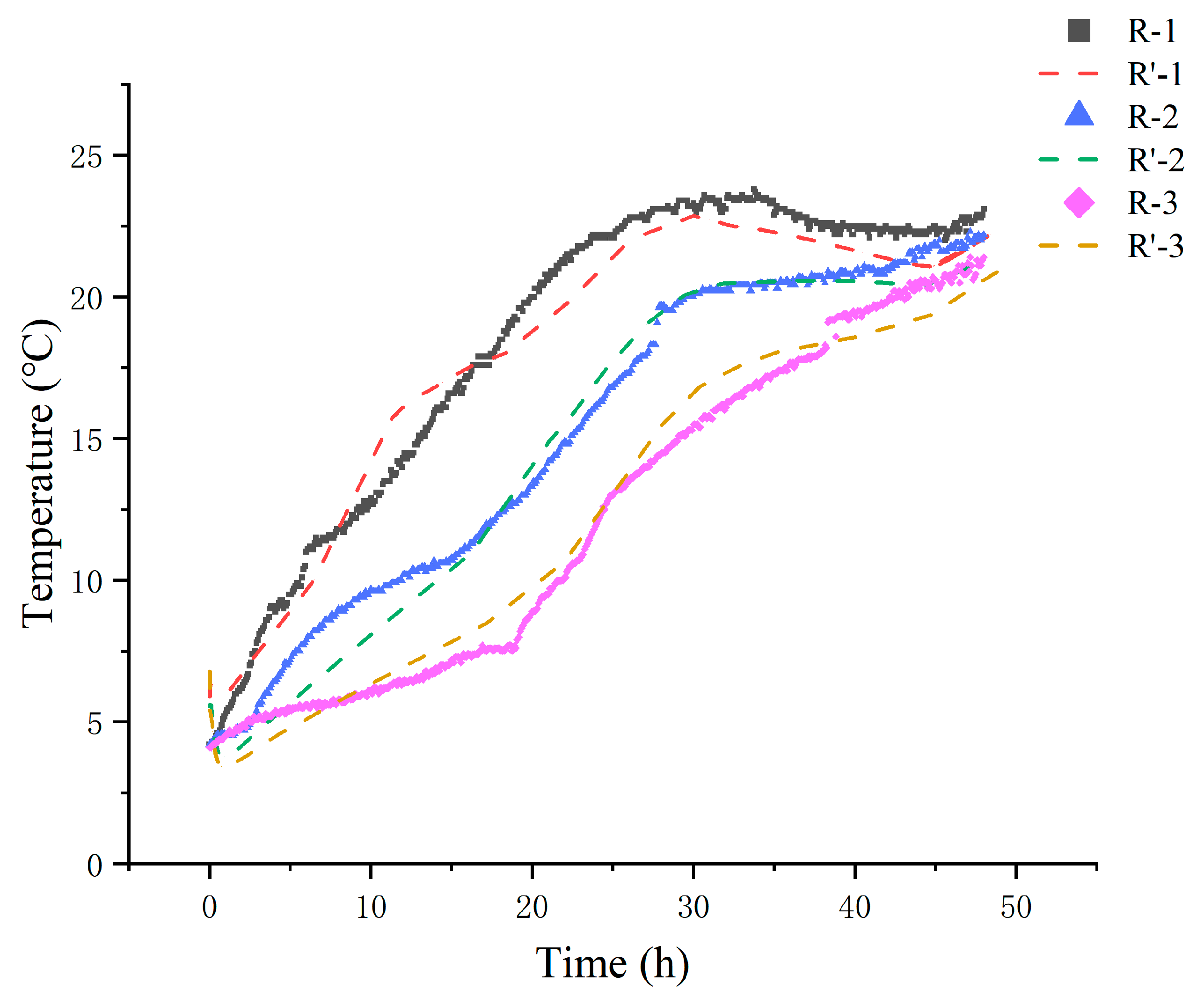
The National Shellfish Sanitation Program (NSSP) recommends that live shellfish should be stored in an environment kept at or below 7.2 °C using ice or mechanical refrigeration [38]. Monitoring temperature fluctuations during delivery is, therefore, crucial. The temperatures of live clams in the R-1, R-2, and R-3 groups were recorded throughout the delivery process and compared to the simulated values (Figure 2). The internal temperature, initially at 5 °C, increased progressively over time. In the R-1 and R-2 groups, which were supplied with fewer ice packs, the temperature rose rapidly, surpassing the recommended threshold by reaching 7.4 °C within 3 h and 7.2 °C within 5 h. Conversely, the R-3 group, with more ice packs, only reached 7.3 °C after 15 h. As the process continued up to 48 h, temperature stabilization occurred, which led to a reduced temperature differential. By the end of the 48 h period, the measured temperatures of the R-1, R-2, and R-3 groups were 23.1 °C, 22.2 °C, and 21.4 °C, respectively.
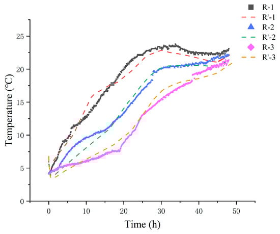
Figure 2.
Comparison of experimental (R-) and simulated (R’-) internal temperatures of different treatments. R-1 is the group with one ice pack, R-2 is the group with two ice packs, and R-3 is the group with three ice packs.
A comparison between the simulated and experimental values (Figure 2) shows strong alignment. Across all groups, the temperature difference between the experimental and simulated results was generally less than 1.5 °C. This agreement was further quantified by the RMSE coefficient at different times (Table 3), which was within the range of 0.10–0.97 °C, with a gradual decrease observed over time. Slight deviations are observed in the temperature curves during the phase transition period of the ice packs, which is consistent with the research by Pattanaik and Jenamani [39]. Analysis of unstable natural convection is subject to disturbances and boundary condition settings. Factors such as airflow and heat conduction cause non-uniform heat transfer, condensation, deformation, and changes in ice pack contact conditions with the insulation material. Overall, the results indicate that the heat transfer model well represented the temperature distribution in the box with satisfactory accuracy.
Table 3.
RMSE coefficients of predicted and measured temperatures at different times.
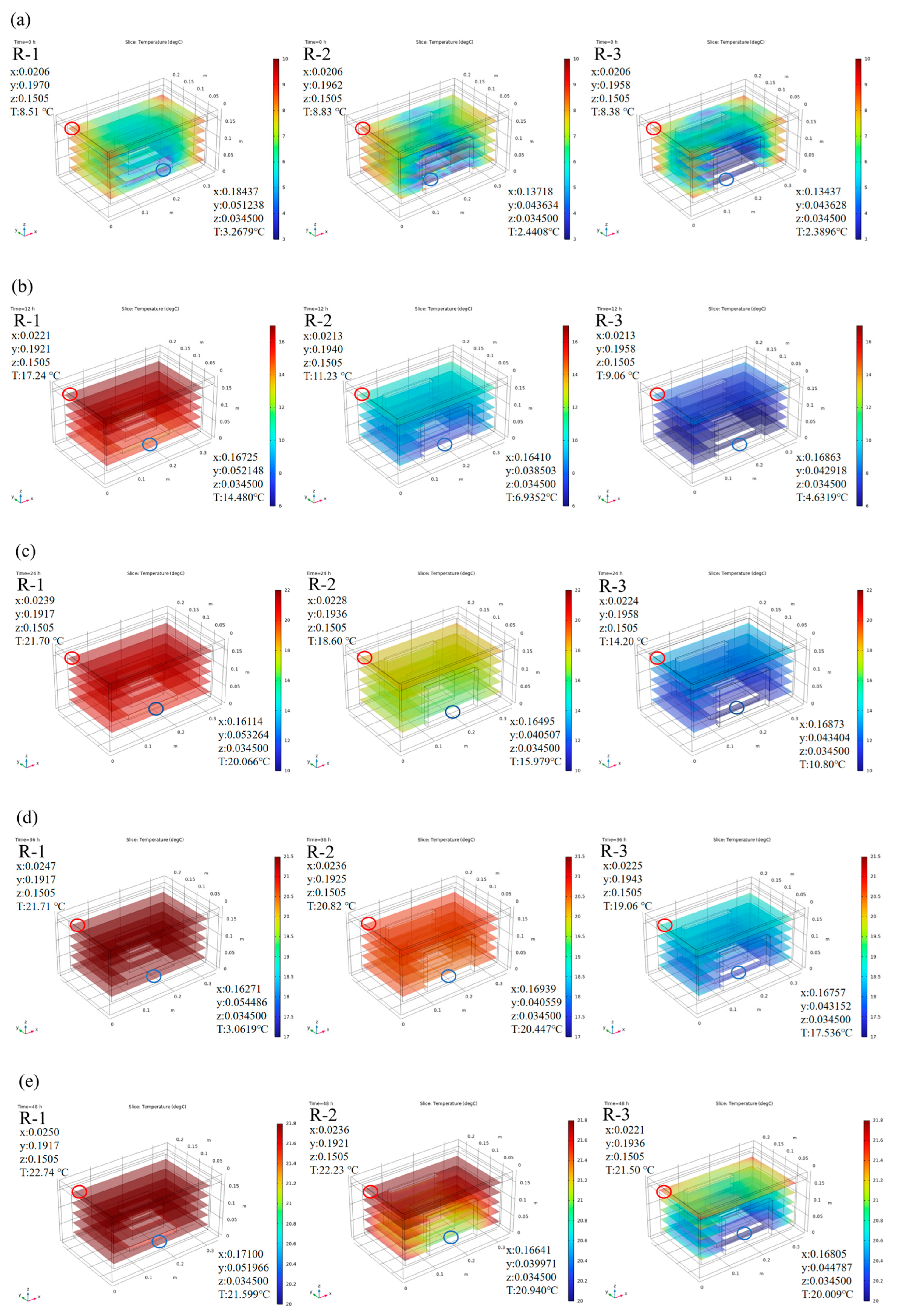
Based on the model calculations, we analyzed the effect of different packing schemes. Figure 3 shows the predicted temperature distribution in the R-1, R-2, and R-3 groups during cold chain breakage, where red presents higher temperatures and blue indicates lower temperatures. Considering that all ice packs were positioned near the bottom of the box, slightly lower temperatures at the bottom were observed due to direct contact between the samples and the ice packs. As expected, the addition of more ice packs resulted in greater cold air release, leading to lower temperatures at any given time point. The R-1 group, with only one ice pack positioned at the bottom, exhibited the highest temperatures among all groups. The temperature difference between the groups was most pronounced within the first 24 h. The highest temperature area was located at the top interior of the container in the R-1 group, and the lowest temperature area was located at the bottom in the R-3 group. A maximum difference of 10 °C was observed between the R-1 (21.7 °C) and R-3 (10.8 °C) groups at the 24 h mark. As the temperature changes in each group began to stabilize, the temperature gap narrowed; this trend was consistent with the earlier temperature curves.
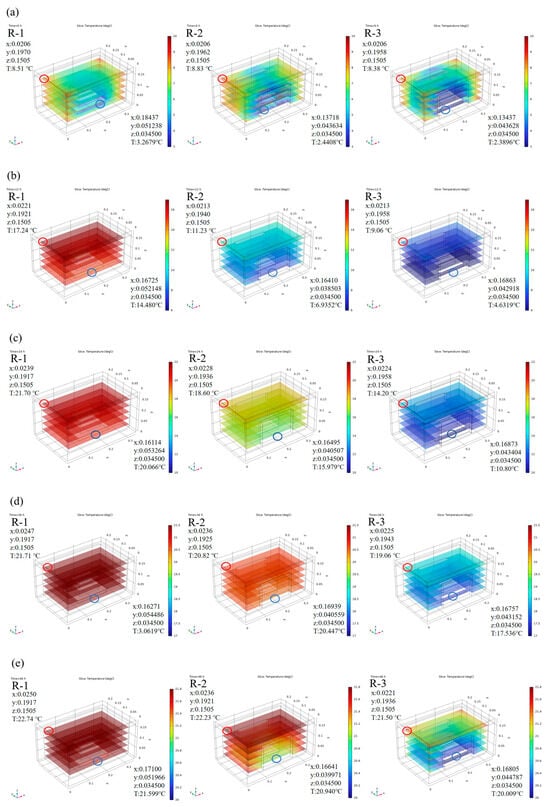
Figure 3.
Predicted internal temperature distribution of different groups at 0 h (a), 12 h (b), 24 h (c), 36 h (d), and 48 h (e). R-1 is the group with one ice pack, R-2 is the group with two ice packs, and R-3 is the group with three ice packs. The red circle indicates the location of hot spots, and the blue circle indicates the location of cold spots.
Meanwhile, the temperature distribution within the container was not uniform, and “hot spots” were noticed, which were further investigated to understand their behavior. Due to the regular symmetry of the model, hot spots were evenly distributed in the four corners of the top interior of the container. For detailed analysis, one corner was taken as a representative example. In the R-1 group, the temperature in the hot spot increased to 21.70 °C at 24 h, while that for the R-3 group was only 14.20 °C. Movement of hot spots over time was also noted. For instance, in the R-1 group, the hot spot initially started in the corner with coordinates 0.0206, 0.1970, 0.1505 and a temperature of 8.51 °C. It gradually shifted toward the center and eventually reached 22.74 °C at coordinates 0.0250, 0.1917, 0.1505 by 48 h. In comparison, the hot spots of the groups with fewer ice packs were positioned closer to the center, while in groups with more ice packs, the hot spots remained near the corners. For example, the hot spots in the R-1, R-2, and R-3 groups were located at 0.0247, 0.1917, 0.1505; 0.0236, 0.1925, 0.1505; and 0.0225, 0.1943, 0.1505, with corresponding temperatures of 21.71 °C, 20.82 °C, and 19.06 °C at 36 h, respectively.
The simulation results provide valuable insights into the temperature distribution of the box, which is critical for optimizing the transportation conditions of live R. philippinarum. By analyzing the temperature field of the box, it is evident that the addition of more ice packs can effectively maintain lower temperatures and restrict the movement of hot spots toward the center, therefore improving uniformity of temperature distribution. This is essential for maintaining the viability and quality of the fresh product.
3.2. Sensory Analysis
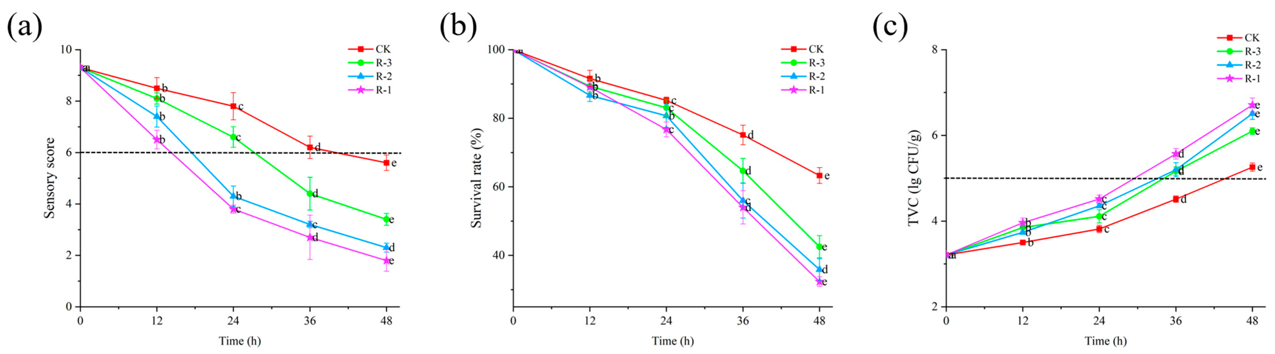
Sensory evaluation serves as the most intuitive indicator of food freshness [40]. As shown in Figure 4a, the sensory scores of live R. philippinarum in each group decreased significantly with the extension of cold chain breakage (p < 0.05). The R-1 group exhibited the most rapid decline in sensory scores, while the R-3 group showed a slower decline. Compared to the CK and R-3 groups, both of which maintained sensory scores above 8, the sensory scores in the R-1 and R-2 groups dropped to 7.4 and 6.5, respectively, after 12 h. At 24 h, the sensory scores in the R-1 and R-2 groups dropped below the rejection limit, reaching 3.8 and 4.3, respectively. As delivery extended, even the CK group, which was stored at 4 °C, experienced a decline in sensory scores below the sensory rejection limit, reaching 5.6 at 48 h. At that time, the R-3 group still exhibited a sensory score of 3.4, while rapid deterioration was observed in the R-1 and R-2 groups, with significantly low scores of 1.8 and 2.3, respectively (p < 0.05). The sensory quality of live R. philippinarum deteriorated to varying degrees due to the action of enzymes and microorganisms [41], and temperature fluctuations can further accelerate deterioration of the sensory quality of clams. These results align with findings by Li et al. [42], who reported that low temperatures can better maintain the overall sensory freshness of razor clams.
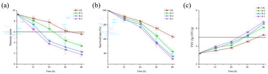
Figure 4.
Effects of different packaging treatments on the sensory score (a), survival rate (b), and TVC (c) of live clams during delivery. Different letters indicate significant differences between different times for the same treatment (p < 0.05). CK is the control group, which was stored at 4 °C. R-1 is the group with one ice pack, R-2 is the group with two ice packs, and R-3 is the group with three ice packs, all of which were stored at 25 °C.
3.3. Survival Rate
The survival rate can directly reflect the overall freshness of R. philippinarum. As shown in Figure 4b, the initial survival rate of R. philippinarum in all groups was 100%. With delivery time extension, the survival rate exhibited a gradual decline initially, followed by a more rapid decrease in the later stages (p < 0.05), with higher mortality observed in groups with fewer ice packs. This indicates that a slow change of temperature is beneficial for improving the survival rate of aquaculture products [43]. During the first 12 h, there was no significant difference in survival rates among the groups. By the 24 h mark, the survival rates of the CK and R-3 groups remained above 83%, whereas those of the R-1 and R-2 groups dropped to 76.72% and 80.72%, respectively. As time progressed, increasing temperatures stimulated the activity of spoilage bacteria and enzymes, accelerating mortality of the shellfish [44]. After 48 h, the survival rates of the R-1 and R-2 groups, which had fewer ice packs and were exposed to higher temperatures, dropped significantly, to 32.33% and 35.84%, respectively.
3.4. Microbiological Analysis
Microbial proliferation is a major factor contributing to the spoilage of aquatic products. According to the U.S. Food and Drug Administration (FDA) microbial standard [45], the threshold for Total Viable Count (TVC) in shellfish is set at 5 × 10⁵ CFU/g. As illustrated in Figure 4c, the TVC in all four groups of R. philippinarum exhibited a continuous increase throughout the delivery period. Compared to the initial TVC for the sample, that is 3.21 lg CFU/g, the TVC of the CK reached 3.82 log CFU/g after 24 h, while the R-1, R-2, and R-3 groups showed slightly higher values of 4.51 log CFU/g, 4.35 log CFU/g, and 4.11 log CFU/g, respectively. As the delivery time progressed, internal temperatures within the packaging gradually increased, which created favorable conditions for bacterial growth. This result is consistent with the findings of Fernandez-piquer et al. [46], who reported that high temperatures during live oyster storage can lead to an increase in TVC, decreasing product shelf life. By the 48 h mark, the TVC levels had increased significantly in all groups, reaching 5.26, 6.71, 6.51, and 6.10 log CFU/g for the CK, R-1, R-2, and R-3 groups, respectively. All values exceeded the FDA limit of 5 × 10⁵ CFU/g. Notably, the R-1 group, which contained fewer ice packs, recorded the highest TVC at 6.71 log CFU/g, surpassing the other groups. Bernardez and Pastoriza [47] reported that elevated temperatures, along with the accumulation of waste or decomposition products from dead mussels within containers, promote microbial growth. This finding aligns with our survival rate results. Furthermore, these outcomes are consistent with the study by Love et al. [48], which demonstrated that cold chain management can effectively inhibit the growth of Vibrio parahaemolyticus in live oysters.
3.5. Physical and Chemical Analysis
3.5.1. WHC
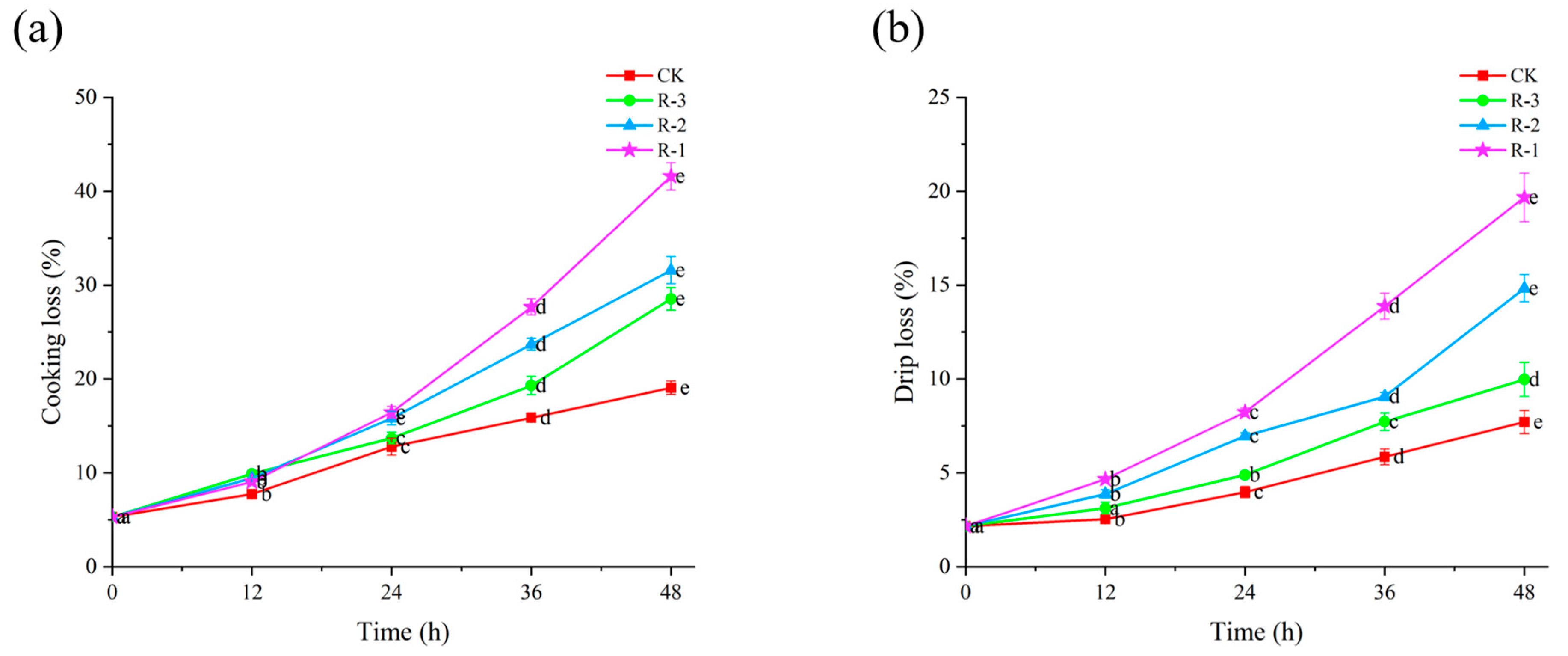
Cooking loss and drip loss can reflect the ability of shellfish to retain their intrinsic water content during delivery [49]. Figure 5 shows the cooking and drip loss of the four groups. Initially, the cooking loss and drip loss for live samples were measured at 5.32% and 2.16%, respectively. With the extension of delivery time, both cooking loss and drip loss increased significantly (p < 0.05). As seen in Figure 5a, within the first 24 h, cooking loss in the CK (3.97%) and R-3 (4.89%) groups remained below 5%, while the R-1 and R-2 groups recorded higher values of 8.23% and 6.95%, respectively. However, cooking loss rose sharply to 19.07%, 41.63%, 31.58%, and 23.53% for the CK, R-1, R-2, and R-3 groups at 48 h, respectively (p < 0.05). Among the groups, R-1, which contained fewer ice packs, experienced the most rapid temperature increase, resulting in the highest cooking loss. The rise in temperature during delivery contributed to structural degradation of muscle cells, leading to increased water loss and a consequent decline in overall quality [50].
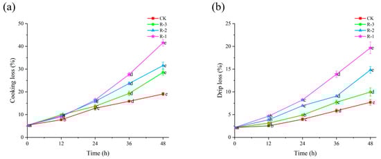
Figure 5.
Effects of different packaging treatments on cooking loss (a) and drip loss (b) of live clams during delivery. Different letters indicate significant differences between different times for the same treatment (p < 0.05). CK is the control group, which was stored at 4 °C. R-1 is the group with one ice pack, R-2 is the group with two ice packs, and R-3 is the group with three ice packs; all were stored at 25 °C.
As shown in Figure 5b, the trends for drip loss followed a pattern similar to that observed for cooking loss. The CK group exhibited relatively lower drip loss, while the R-1 group showed the highest and most rapid increase. In the first 12 h, the drip loss in all groups remained below 5%. However, the drip loss in the R-1 and R-2 groups increased significantly to 19.67% and 14.83% after 48 h delivery, respectively, while that for the CK and R-3 groups remained under 10%. This sharp increase in drip loss is likely due to the reduction in ice packs leading to a rise in temperature, which in turn significantly accelerated proteolysis and degradation of the muscle structure, leading to tissue collapse and a subsequent decline in WHC [51,52].
3.5.2. pH
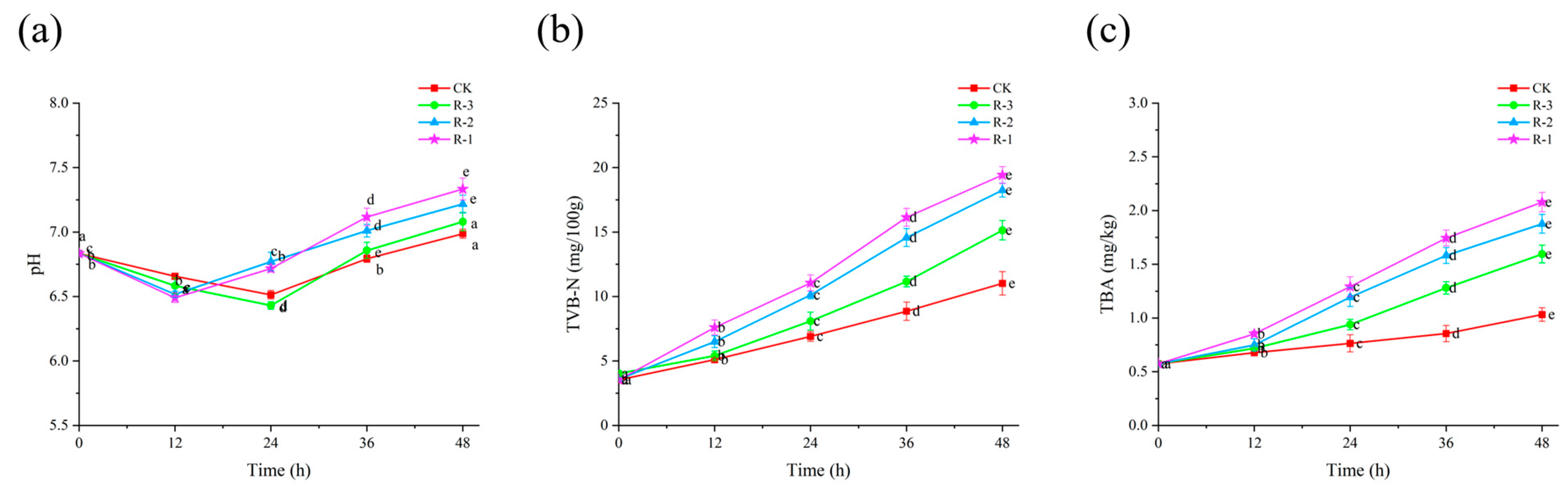
Microbial growth and subsequent protein degradation lead to an increase in pH, making it a valuable indicator of the freshness of R. philippinarum [53]. As shown in Figure 6a, the initial pH of live R. philippinarum was 6.83, followed by a slight decline before rising again as delivery time extended. The inflection points of pH changes varied between groups. The pH values of the R-1 and R-2 groups reached their lowest values (6.49 and 6.52, respectively) at 12 h, but then rapidly increased to 7.33 and 7.22 by 48 h. In contrast, the lowest pH values for the CK and R-3 groups appeared at 24 h (6.51 and 6.43), and their pH values increased more slowly, reaching 6.99 and 7.08 at 48 h, respectively. This can be explained by the use of more ice packs ensuring lower temperatures throughout cold chain logistics, therefore suppressing the production of alkaline substances from microbial activity [54].
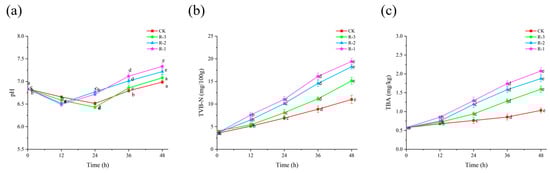
Figure 6.
Effects of different packaging treatments on the pH (a), TVB-N (b), and TBA (c) of live clams during delivery. Different letters indicate significant differences between different times for the same treatment (p < 0.05). CK is the control group, which was stored at 4 °C. R-1 is the group with one ice pack, R-2 is the group with two ice packs, and R-3 is the group with three ice packs; all were stored at 25 °C.
3.5.3. TVB-N
Protein degradation leads to the accumulation of volatile basic nitrogenous compounds, and TVB-N is a reliable indicator of freshness in aquatic products [55]. As shown in Figure 6b, the initial TVB-N value of the live R. philippinarum samples was only 3.54 mg/100 g. With the extension of delivery time, the TVB-N levels increased significantly (p < 0.05), showing a slow rise initially followed by a rapid increase during the later stages of delivery. In the first 12 h, no significant differences were observed among the groups, with all TVB-N values remaining under 8 mg/100 g. This observation aligns with findings from [56], which reported that low temperatures limit the accumulation of TVB-N by inhibiting microbial activity and reducing enzyme activity. Consequently, only small amounts of amines were produced during this period. However, after 36 h, the R-1 group exhibited the highest TVB-N levels, reaching 16.14 mg/100 g. By 48 h, the TVB-N values for the CK, R-1, R-2, and R-3 groups were 11.02, 19.42, 18.25, and 15.13 mg/100 g, respectively. Notably, all groups except CK exceeded the national standard for marine shellfish (TVB-N ≤ 15 mg/100 g) [57]. This rise in TVB-N is largely attributable to metabolites produced by spoilage bacteria that induce protein degradation. Although low temperatures may not completely prevent the increase in TVB-N, they can significantly slow bacterial proliferation and delay protein degradation, as observed in [58].
3.5.4. TBA
TBA is a key indicator of lipid oxidation [59]. Compared to the initial TBA value of live R. philippinarum (0.57 mg/kg), shown in Figure 6c, the TBA values of all the groups all increased along with extension of the delivery period (p < 0.05). Within the first 24 h, the TBA values in the R-1 and R-2 groups had already surpassed 1 mg/kg, reaching 1.29 mg/kg and 1.19 mg/kg, respectively. In contrast, the CK and R-3 groups exhibited lower TBA values of 0.76 mg/kg and 0.94 mg/kg. At 48 h, the TBA values of the CK, R-1, R-2, and R-3 groups reached 1.31, 2.08, 1.88, and 1.59 mg/kg, respectively, all of which exceeded the critical threshold for spoilage in aquatic products (1.0 mg/kg) [60]. Studies on mussels (Perna canaliculus) [61] and Pacific oysters (Crassostrea gigas) [62] have shown that elevated temperatures exacerbate unsaturated fatty acid metabolism, leading to accelerated lipid oxidation and the development of off-odors.
3.6. Color Measurements
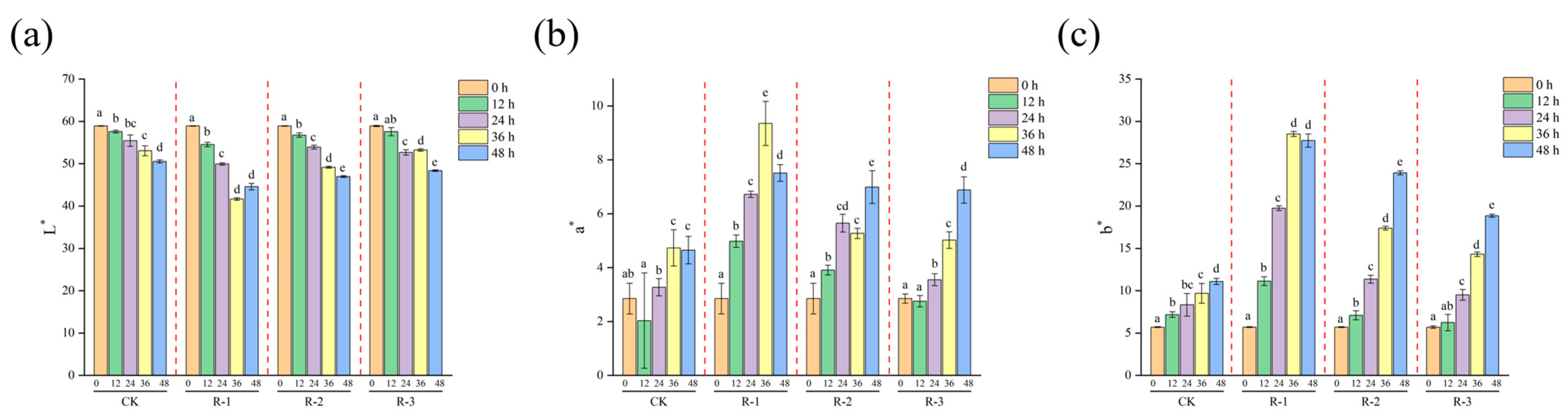
Color is a key quality attribute that consumers often associate with taste and overall product quality [63]. As presented in Figure 7, a significant decline in L* values (p < 0.05) was observed with prolonged delivery time, alongside a significant increase in a* and b* values (p < 0.05). Overall, the color differences in the R-1 and R-2 groups were more pronounced during the delivery period, whereas the CK and R-3 groups showed minimal color variation, indicating that having fewer ice packs exacerbated the color changes. Specifically, the L* value in the R-1 group significantly decreased from 58.91 to 41.65, while the a* value increased from 2.85 to 9.35 and the b* value increased sharply from 5.69 to 28.51 after 36 h. In contrast, the R-3 group exhibited more stable color changes, with L* decreasing to 48.37, and the a* and b* values increasing to 6.88 and 18.85 at 48 h, respectively. Color changes are influenced by pigment activity, protein denaturation, the presence of bioactive compounds [64], and hormonal regulation related to environmental stress [65], which can be accelerated by elevated temperatures; therefore, maintaining a low-temperature environment effectively inhibited color changes in live R. philippinarum.
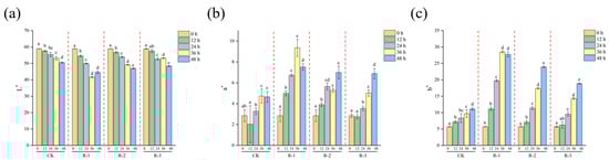
Figure 7.
Effects of different packaging treatments on the color parameters L* (a), a* (b), and b* (c) during delivery. Different letters indicate significant differences between different times for the same treatment (p < 0.05). CK is the control group, which was stored at 4 °C. R-1 is the group with one ice pack, R-2 is the group with two ice packs, and R-3 is the group with three ice packs; all were stored at 25 °C.
3.7. Texture Properties
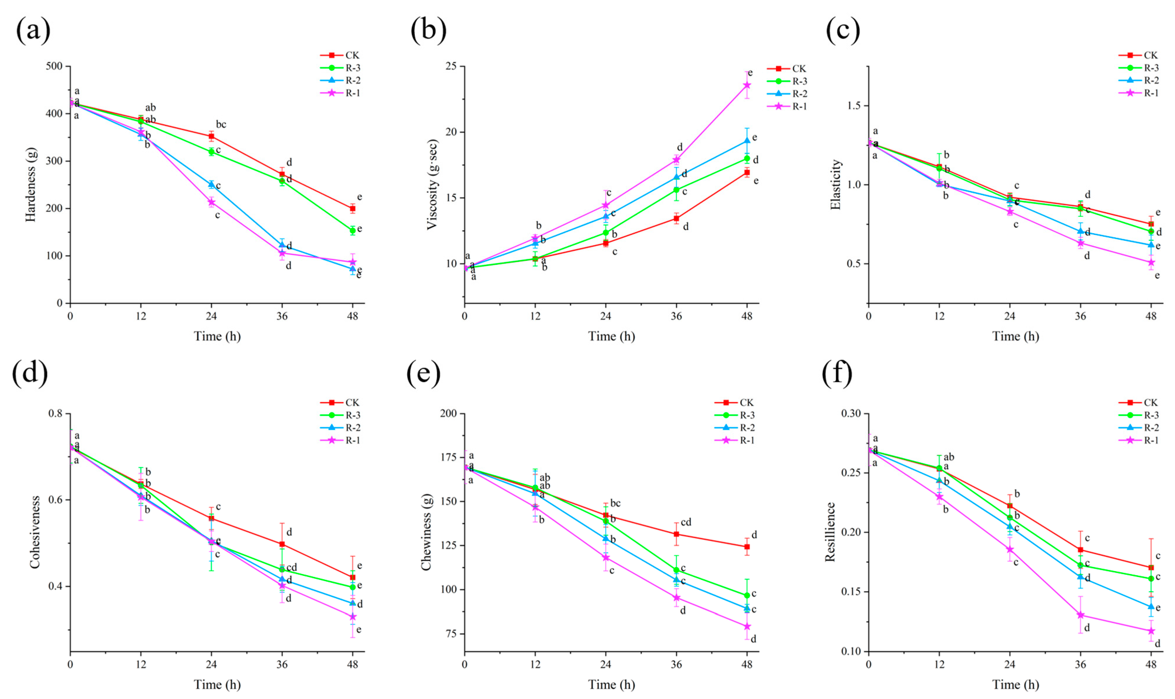
As shown in Figure 8, the hardness, elasticity, cohesiveness, chewiness, and resilience of the samples significantly decreased (p < 0.05), while viscosity significantly increased (p < 0.05), as delivery progressed. The higher the sample temperature, the more change occurred in texture properties. Groups with higher internal temperatures exhibited more pronounced changes in these textural parameters.
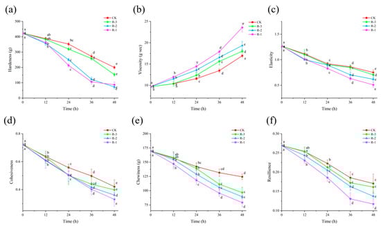
Figure 8.
Effects of different packaging treatments on the texture properties of hardness (a), viscosity (b), elasticity (c), cohesiveness (d), chewiness (e), and resilience (f) during delivery. Different letters indicate significant differences between different times for the same treatment (p < 0.05). CK is the control group, which was stored at 4 °C. R-1 is the group with one ice pack, R-2 is the group with two ice packs, and R-3 is the group with three ice packs; all were stored at 25 °C.
Hardness, in particular, is a key index reflecting the internal binding force that allows food to maintain its structure [66]. As shown in Figure 8a, compared with the initial hardness value of the sample (423.29 g), the decrease in hardness was minor during the first 12 h, with all groups maintaining values above 350 g. However, a rapid decline occurred thereafter, especially the hardness in the R-1 and R-2 groups, which significantly fell below 250 g at 24 h, with R-3 maintaining a slightly higher value of 319.41 g. After 48 h, the hardness values in the CK, R-1, R-2, and R-3 groups dropped significantly to 199.73, 76.84, 92.50, and 153.17 g, respectively (p < 0.05). Figure 8c–f show that the changes in elasticity, cohesiveness, chewiness, and resilience followed a pattern similar to that of hardness, with all exhibiting a significant downward trend (p < 0.05). After 48 h, the elasticity in the CK, R-1, R-2, and R-3 groups decreased from an initial value of 1.267 to 0.752, 0.508, 0.618, and 0.705, respectively (p < 0.05), and the cohesiveness decreased from 0.722 to 0.421, 0.331, 0.361, and 0.398 in the CK, R-1, R-2, and R-3 groups, respectively (p < 0.05). Similarly, the chewiness and resilience of the CK group remained the highest, while the R-1 group experienced the greatest decline. However, the trends in viscosity were different. As shown in Figure 8b, the viscosity of the test groups was higher than that of the CK group, and the R-1 group exhibited the most rapid changes. After 24 h, the viscosity values for the R-1, R-2, and R-3 groups were 14.458, 13.59, and 12.358 g·s, respectively, while that of the CK group remained below 12 g·s. The viscosity values in the CK, R-1, R-2, and R-3 groups significantly increased to 15.94, 23.57, 19.34, and 18.00 g·s at 48 h, respectively (p < 0.05). These alterations can be attributed to the denaturation and aggregation of muscle proteins at elevated temperatures, leading to progressive softening of the tissue structure [67,68].
3.8. Water Distribution Analysis
LF-NMR can quickly and non-destructively determine the water state and fluidity in aquatic products [69], and MRI can directly obtain visualization image information from the sample.
3.8.1. LF-NMR Analysis
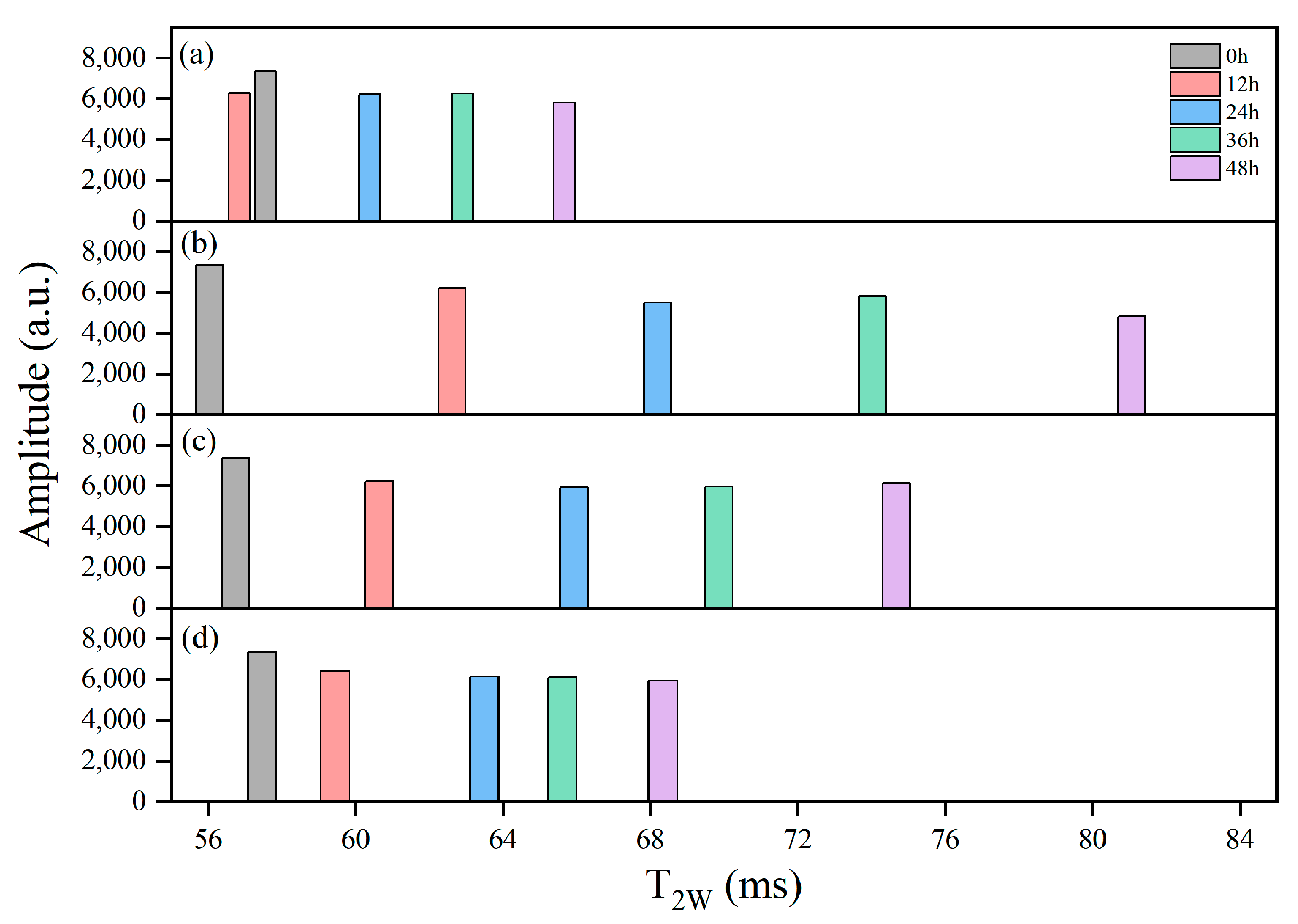
LF-NMR was employed to assess moisture status and mobility of the samples. As shown in Figure 9, T2W generally increased with extended delivery time, and the groups experienced higher internal temperatures that corresponded to greater T2W values. After 48 h, the T2W of the R-1 and R-2 groups increased to 78.85 ms and 73.18 ms, respectively, compared to 64.98 ms in the CK group. In contrast, the R-3 group, which maintained a lower temperature, effectively slowed down water mobility, and exhibited a T2W of 67.56 ms, closely resembling the CK group.

Figure 9.
Distribution of single-component relaxation time (T2w) spectra for the CK (a), R-1 (b), R-2 (c), and R-3 (d) groups during delivery.
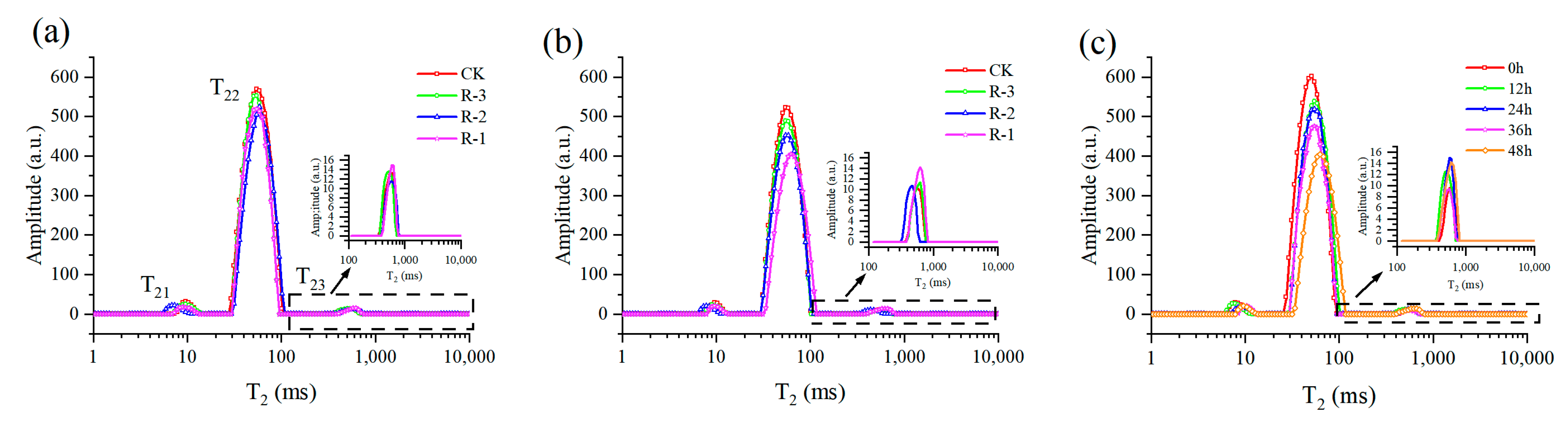
Figure 10 showed the multicomponent relaxation distribution (T2) of the four groups during delivery. Overall, three relaxation peaks were observed and named as peak T21, T22, T23, suggesting three water populations with different proton mobilities. The shorter the T2 is, the lower the mobility of water fraction is, and the faster relaxation is, or vice versa. The T21 peak (1–10 ms) was normally considered to represent the bound water, which was tightly associated with macromolecules. The protons of water trapped within the myofibrillar protein network were shown in the T22 peak, which is the dominant relaxing component, ranging from 10 to 100 ms. Meanwhile, the T23 peak (100–1000 ms) was related to the water outside the myofibrillar lattice and muscle cells [70].

Figure 10.
Distribution of multicomponent relaxation spectra (T2) for all four groups at 24 h (a) and 48 h (b), and for the R-1 group (c) during transport. CK is the control group, which was stored at 4 °C. R-1 is the group with one ice pack, R-2 is the group with two ice packs, and R-3 is the group with three ice packs; all were stored at 25 °C.
Almost no shift occurred in the T2 relaxation distribution of the four groups at 24 h, as shown in Figure 10a; however, the transverse relaxation distribution exhibited a significant rightward shift, especially the T22 peak, after 48 h (Figure 10b). The rightward shift of the T22 peak was more pronounced in the R-1 and R-2 groups compared to the CK group, demonstrating the increased water mobility of samples experiencing higher temperatures. Taking the R-1 group, for instance (Figure 10c), with extension of delivery time, the T2 relaxation distribution gradually shifted to the right, and the amplitude of the T22 peak obviously decreased, suggesting an increase of water mobility and a reduction in the immobilized water population.
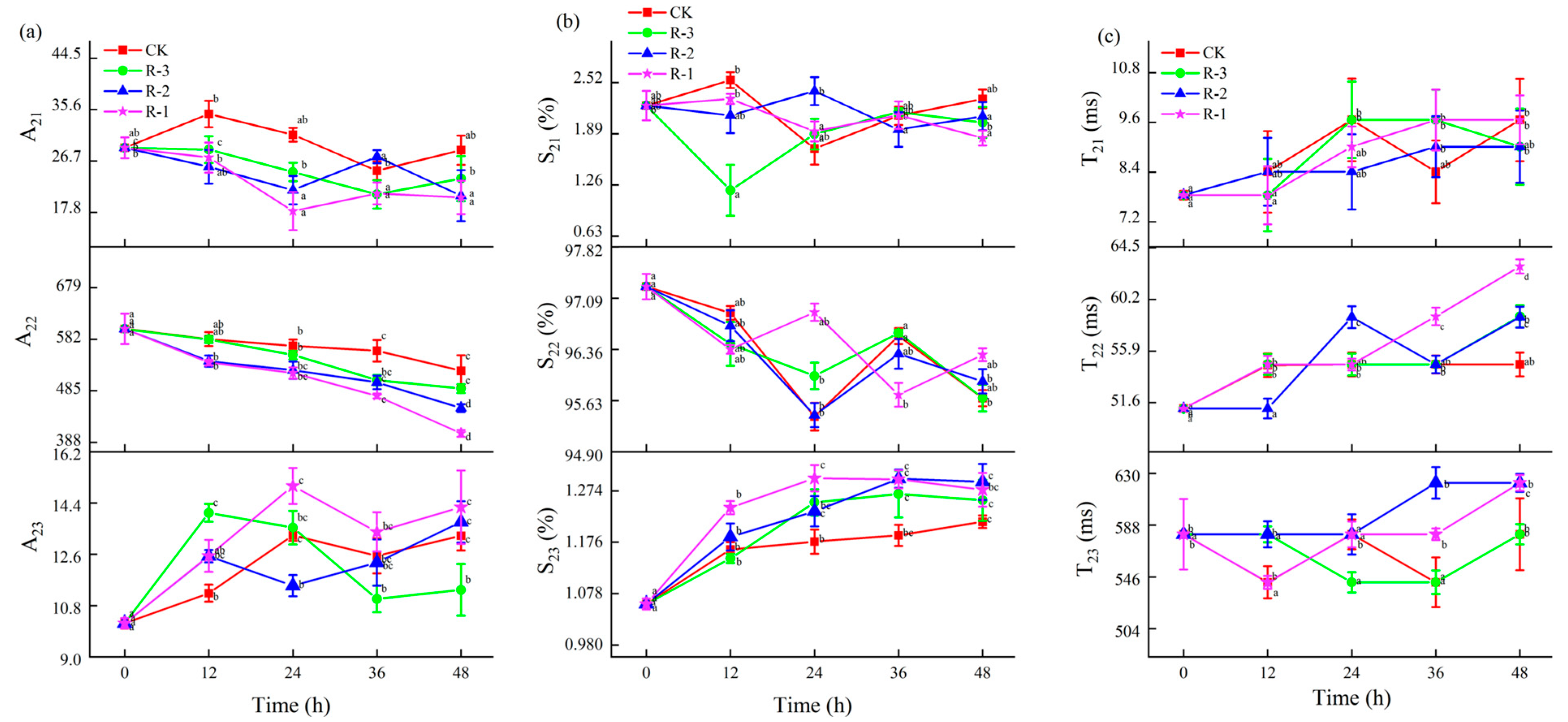
The changes in the T21, T22, and T23 relaxation time constants, relative peak proportions (S21, S22, and S23), and peak areas (A21, A22, and A23) for the samples under different treatments were further analyzed, as shown in Figure 11. Changes in T21, A21, and S21 values were not obvious among the R-1, R-2, and R-3 groups compared to the CK group, suggesting that the binding strength between water and macromolecules remained relatively stable during delivery. However, as shown in Figure 11a,b, both the relative peak proportion (S22) and the peak area (A22) of the immobilized water showed overall decreasing trends along with the extension of delivery time, while S23 and A23, corresponding to free water, increased. Among the test groups, the R-3 group exhibited the smallest changes in S2i and A2i, demonstrating a pattern more similar to the CK group, while the R-1 group demonstrated the most pronounced change. Taking A22 for instance, A22 significantly decreased from 601.35 to 522.62, 489.16, 452.30, and 404.85 in the CK, R-3, R-2, and R-1 groups after 48 h of transport, respectively (p < 0.05), while A23 significantly increased from 10.18 to 13.25, 11.35, 13.74, and 14.25 in the CK, R-3, R-2, and R-1 groups. The changes in A22 and A23 confirmed the dynamic changes in the water proton populations; that is, immobilized water transferred into free water during transport. As shown in Figure 11c, the T22 time constant for each treatment showed an increase. At 24 h, the T22 values of the R-1 and R-3 groups were similar to that of the CK group (54.79 ms), whereas the R-2 group had a slightly higher value of 58.73 ms. At the end of the transport period (48 h), the R-1 group demonstrated a pronounced change compared to the CK group, and the T22 values of the CK, R-1, R-2, and R-3 groups were 54.79 ms, 62.95 ms, 58.73 ms, and 58.79, respectively, showing an increase in water mobility. Compared to the CK and R-3 groups (541.59 ms), the T23 values for the R-1 and R-2 groups at 36 h were much higher, at 580.52 ms (R-1) and 622.26 ms (R-2), respectively. At 48 h, the T23 values for the R-1 and R-2 groups had all increased to 622.26 ms, which was significantly higher than that of the CK and R-3 groups (580.52 ms). This finding is consistent with a report by Sánchez-Valencia et al. [71], which noted that the relative abundance of immobilized water in hake decreased as delivery time increased. This phenomenon indicated that the trapped water was altered to free water during delivery, due to the destruction of myofibril structure [72], while sustained low temperatures hindered excessive water loss by slowing muscle fiber degradation.
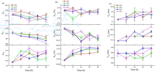
Figure 11.
Changes in the relaxation parameters A2i (a), S2i (b), and T2i (c) in the different groups during delivery. Different letters indicate significant differences between different times for the same treatment (p < 0.05). CK is the control group, which was stored at 4 °C. R-1 is the group with one ice pack, R-2 is the group with two ice packs, and R-3 is the group with three ice packs; all were stored at 25 °C.
3.8.2. MRI Analysis
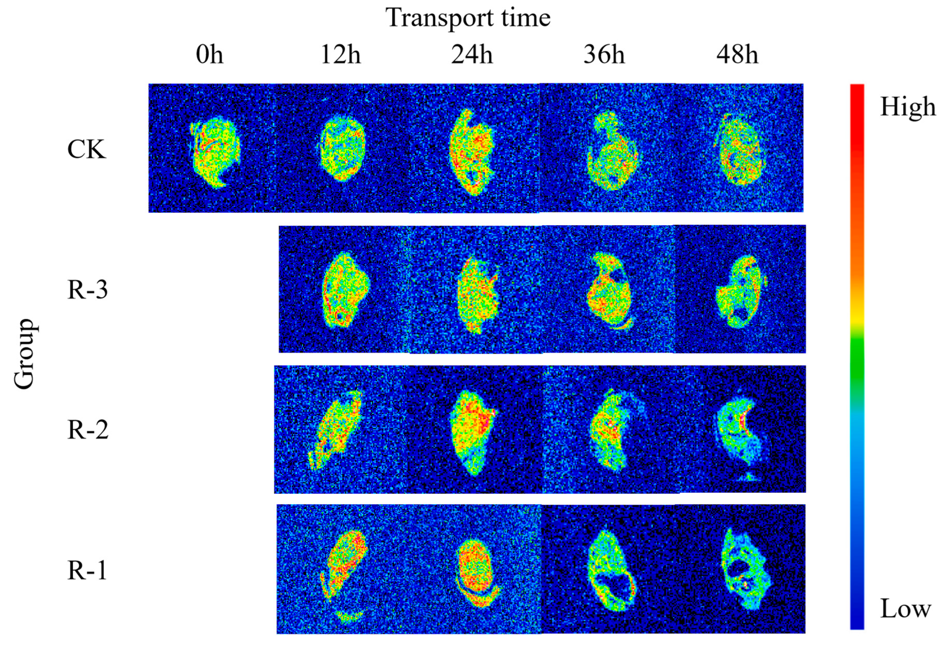
MRI was employed to visualize the water distribution, and the pseudo-color proton density-weighted images are displayed in Figure 12. The image contrast is dominated by the number of detectable protons in the voxel, and red areas indicate a higher density of hydrogen protons, signifying higher moisture content, while blue areas represent lower proton density, and therefore lower moisture content [73].
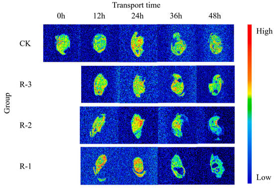
Figure 12.
Proton density–weighted images of live clams in different packaging groups during delivery. CK is the control group, which was stored at 4 °C. R-1 is the group with one ice pack, R-2 is the group with two ice packs, and R-3 is the group with three ice packs; all were stored at 25 °C.
The T2-weighted image of CK appeared yellowish-green, reflecting a low proton signal and minimal water fluidity. However, visible color changes were observed as the transport time increased, and the variation was more pronounced for the groups with fewer ice packs. As shown in the pseudo-color images for groups R-1 and R-2 at 12 h, the water distribution inside the samples became uneven, and the enhanced proton signal resulted in more prominent red and yellow regions.
As the transport time extended from 12 to 24 h, the pseudo-color images showed a significant expansion in red regions across the sample sections. The R-1 and R-2 groups exhibited markedly larger red regions compared to the CK group, indicating a more pronounced rise in free water content and further highlighting the uneven water distribution throughout the sample. Particularly, the proton density in the 36–48 h pseudo-color images of the R-1 and R-2 groups showed a declining trend from the edge toward the center of the samples, and the colors progressively darkened to blue-green. During this period, significant water loss occurred in the muscle tissue, leading to a weakening of the signal intensity on the MRI images. This decrease may be due to the breakdown and denaturation of muscle proteins [74]. Meanwhile, as delivery time extended, formation of cavities in the pseudo-color images of the sample cross-sections was observed, especially in the samples exposed to higher temperatures. This might be related to the action of an endogenous protease that degrades isolated myofibrils, causing more rapid breakdown of the structures and thus the formation of the cavities [75]. Notably, the pseudo-color images of the R-3 group, which maintained a low temperature after 48 h, remained more similar to those of the CK group, suggesting that the quality of the R-3 group was better preserved.
3.8.3. Correlation Analysis Between LF-NMR and Physicochemical Properties
Pearson correlation analysis was conducted to examine the relationship between LF-NMR measurements and physicochemical properties, and the results are presented in Figure 13 and Table A1. Positive or negative values indicate the direction of the correlation between the indicators, while the absolute values represent the strength of these correlations.
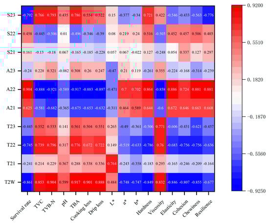
Figure 13.
Pearson correlations between quality characteristics and LF-NMR relaxation.
The survival rate was found to be negatively correlated with T2W (r = −0.861 *), T22 (r = −0.745 *), and S23 (r = −0.792 *) (p < 0.05), but positively correlated with A22 (r = 0.904 **) (p < 0.01). Additionally, TVC, TVB-N, and TBA were significantly negatively correlated with A22 (r = −0.888 **, r = −0.921 **, and r = −0.917 **), while being positively or significantly positively correlated with T2W (r = 0.853 *, r = 0.904 **, and r = 0.917 **) and S23 (r = 0.766 *, r = 0.793 *, and r = 0.786 *). Moreover, TBA exhibited a positive correlation with T22 (r = 0.776 *).
WHC showed a strong correlation with LF-NMR. Both cooking loss and drip loss were significantly positively correlated with T2w (r = 0.901 **, r = 0.888 **) (p < 0.01) and negatively correlated with A22 (r = −0.883 **, r = −0.897 **) (p < 0.01). In addition, drip loss was positively correlated with T22 (r = 0.722 *) (p < 0.05).
With regard to texture properties, hardness exhibited significant positive correlations with A22 (r = 0.864 **) and S23 (r = 0.721 *) (p < 0.05 or p < 0.01). However, hardness was negatively correlated with T2w (r = −0.849 *) and T22 (r = −0.786 *) (p < 0.05). Viscosity demonstrated a positive correlation with T2W (r = 0.832 *), T22 (r = 0.760 *) and T23 (r = 0.771 *) (p < 0.05), while negatively correlating with A22 (r = −0.858 *) (p < 0.05). Elasticity showed a significant positive correlation with A22 (r = 0.886 **) (p < 0.01) and a negative correlation with T2w (r = −0.846 *) (p < 0.05). Cohesion was negatively correlated with T2w (r = −0.807 *) and T22 (r = −0.756 *) (p < 0.05). Chewiness was significantly positively correlated with A22 (r = 0.881 **) (p < 0.01) and negatively correlated with T2w (r = −0.855 *) and T22 (r = −0.756 *) (p < 0.05). Resilience also demonstrated a significant positive correlation with A22 (r = 0.881 **) (p < 0.01) and a negative correlation with S23 (r = −0.776 *) (p < 0.05). In contrast, among the color indices, only the a* and b* values exhibited negative correlations with T2W (r = −0.748 *, r = −0.747 *, respectively) (p < 0.05), while the L* value was positively correlated with T21. These findings are similar to those reported by Tan et al. [76] and Xie et al. [77], suggesting that LF-NMR can serve as a reliable tool for monitoring the physicochemical changes and quality deterioration of R. philippinarum during delivery.
4. Conclusions
The results from this study indicate that different packaging treatments significantly influence the quality of anhydrously preserved live R. philippinarum during disruption in the “last mile” of the cold chain. The study revealed significant variations in temperature field distribution according to the different packaging treatments, as assessed by COMSOL Multiphysics®. The R-3 group with three ice packs exhibited the lowest temperatures and restricted the movement of hot spots toward the center. Using different physicochemical indices to assess quality changes in live R. philippinarum with the three packaging treatments, we found that, with the extension of cold chain breakage time, the survival rate and sensory score of live R. philippinarum significantly decreased, while an increasing trend was observed in TVC, TVB-N, TBA, cooking loss, and drip loss. Fewer ice packs, which promotes a faster rise in temperature intensified changes in the above indices. In addition, the texture of live R. philippinarum deteriorated to different degrees; the hardness, elasticity, chewiness, cohesion, and resilience were significantly decreased (p < 0.05), whereas the viscosity was significantly increased (p < 0.05), although small changes occurred in elasticity and resilience. The a* and b* values significantly increased, whereas the L* values decreased. After 48 h, accompanied by severe corruption, the R-1 group turned dark and yellowish. The change in color in the CK group was small, with a changing trend similar to that seen in the R-3 group. Moreover, the water state profile during delivery was characterized by LF-NMR and MRI. The relaxation characteristics of live R. philippinarum demonstrated that T2w increased, and the T22 peak signal amplitude decreased and shifted to the right, indicating that the proportion of bound water decreased, while the proportion of free water increased. The overall change in the regularity of the CK and R-3 groups was small, contrary to that of the R-1 and R-2 groups, which was caused by maintaining a lower temperature. With a decrease in sample quality, the MRI pseudo-color images showed an expansion of red and yellow regions, followed by cavity formation due to tissue collapse and a decrease in proton density due to the high degree of water loss, causing the pseudo-color map to change to blue-green. The relaxation parameters assessed by LF-NMR exhibited good correlation with survival rate, microbial and classical physicochemical indices, color difference, and texture. These findings underscore the fact that using more ice packs, such as in the R-3 group, can not only maintain lower temperature but also reduce losses caused by “last mile” cold chain breakage, providing a reference for optimizing distribution conditions for live R. philippinarum.
Author Contributions
Y.H.: writing—original draft, data curation, visualization. X.X.: investigation, methodology, resources. S.Y.: writing—reviewing and editing. C.L.: resources, visualization. X.W.: conceptualization, project administration, funding acquisition, writing—review and editing. All authors have read and agreed to the published version of the manuscript.
Funding
This work was supported by the grants from the National Key Research and Development Program of China (2022YFF1101104).
Institutional Review Board Statement
Not applicable.
Informed Consent Statement
Informed consent was obtained from all subjects involved in this study.
Data Availability Statement
The original contributions presented in the study are included in the article, further inquiries can be directed to the corresponding author.
Conflicts of Interest
The authors declare no conflicts of interest.
Appendix A
Table A1.
Correlation equations between the LF-NMR relaxation characteristics and physicochemical and quality characteristics.
References
- FAO. The State of World Fisheries and Aquaculture 2024—Blue Transformation in Action; FAO: Rome, Italy, 2024. [Google Scholar]
- National Bureau of Statistics of China. China Statistical Yearbook; National Bureau of Statistics of China: Beijing, China, 2023.
- Zdrojewska, I.; Lebiedzinska, A.; Szefer, P. Selected seafoods as the components of a highly nutritional diet. [Wybrane owoce morza jako skladniki diety o wysokiej wartosci odzywczej]. Rocz. Panstw. Zakl. Hig. 2005, 56, 131–137. [Google Scholar] [PubMed]
- Barrento, S.; Lupatsch, I.; Keay, A.; Christophersen, G. Metabolic rate of blue mussels (Mytilus edulis) under varying post-harvest holding conditions. Aquat. Living Resour. 2013, 26, 241–247. [Google Scholar] [CrossRef]
- Chen, L.; Shi, H.; Zhang, X.; Xue, C.; Nie, C.; Yang, F.; Shao, Y.; Xue, Y.; Zhang, H.; Li, Z. The effect of depuration salinity on the survival, nutritional composition, biochemical responses and proteome of Pacific oyster (Crassostrea gigas) during anhydrous living-preservation. Food Control 2022, 138, 108977. [Google Scholar] [CrossRef]
- Ekanem, E.O.; Achinewhu, S.C. Mortality and quality indices of live West African hard-shell clams (Galatea paradoxa Born) during wet and dry postharvest storage. J. Food Process. Preserv. 2006, 30, 247–257. [Google Scholar] [CrossRef]
- Chen, S.Q.; Zhang, C.H.; Xiong, Y.F.; Tian, X.Q.; Liu, C.C.; Jeevithan, E.; Wu, W.H. A GC-MS-based metabolomics investigation on scallop (Chlamys farreri) during semi-anhydrous living-preservation. Innov. Food Sci. Emerg. Technol. 2015, 31, 185–195. [Google Scholar] [CrossRef]
- Li, M.; Xie, B.S.; Li, Y.X.; Cao, P.H.; Leng, G.H.; Li, C.C. Emerging phase change cold storage technology for fresh products cold chain logistics. J. Energy Storage 2024, 88, 111531. [Google Scholar] [CrossRef]
- Bi, S.J.; Xue, C.H.; Xu, L.L.; Wen, Y.Q.; Wang, L.H.; Li, Z.J.; Liu, H.Y. Physiological Responses of Clam (Ruditapes philippinarum) to Transport Modes with Different Temperatures. J. Ocean Univ. China 2023, 22, 517–526. [Google Scholar] [CrossRef]
- Jiang, P.H.; Qin, X.M.; Fan, X.P.; Zhang, C.F.; Chen, D.J. The impact of anhydrous storage and transportation at ice temperatures on the post-capture viability and quality of Patinopecten yessoensis. J. Agric. Food Res. 2024, 18, 101277. [Google Scholar] [CrossRef]
- Bai, B.; Zhao, K.; Li, X.Z. Application research of nano-storage materials in cold chain logistics of e-commerce fresh agricultural products. Results Phys. 2019, 13, 102049. [Google Scholar] [CrossRef]
- Meng, X.C.; Xie, R.H.; Liao, J.; Shen, X.; Yang, S.C. A cost-effective over-temperature alarm system for cold chain delivery. J. Food Eng. 2024, 368, 111914. [Google Scholar] [CrossRef]
- Youngtae, P.; Siku, K.; Kwangyeol, R. Prediction of Refrigerated Vehicle Environment for Optimization of Cold-Chain Logistics. ICIC Express Lett. Part B Appl. 2023, 14, 193–199. [Google Scholar] [CrossRef]
- Zhao, X.; Pei, L.; Jia, X.; Qu, M.; Zhang, Z.; Wang, Y. Study the Test Method of Temperature and Humidity Monitoring Equipment in the Cold Chain Transportation Process. J. Phys. Conf. Ser. 2023, 2437, 012065. [Google Scholar] [CrossRef]
- Skudlarek, J.G.; Coyle, S.D.; Bright, L.A.; Tidwell, J.H. Effect of Holding and Packing Conditions on Hemolymph Parameters of Freshwater Prawns, Macrobrachium rosenbergii, during Simulated Waterless Transport. J. World Aquac. Soc. 2011, 42, 603–617. [Google Scholar] [CrossRef]
- Teng, X.Y.; Cong, X.H.; Chen, L.P.; Wang, Q.; Xue, C.H.; Li, Z.J. Effect of repeated freeze-thawing on the storage quality of pacific oyster (Crassostrea gigas). J. Food Meas. Charact. 2022, 16, 4641–4649. [Google Scholar] [CrossRef]
- Alfaro, A.C.; Nguyen, T.V.; Mellow, D. A metabolomics approach to assess the effect of storage conditions on metabolic processes of New Zealand surf clam (Crassula aequilatera). Aquaculture 2019, 498, 315–321. [Google Scholar] [CrossRef]
- Huo, Z.M.; Li, Y.; Rbbani, M.G.; Wu, Q.D.; Yan, X.W. Temperature challenge on larvae and juveniles of the Manila clam Ruditapes philippinarum. Aquac. Res. 2018, 49, 1727–1731. [Google Scholar] [CrossRef]
- So, J.H.; Joe, S.Y.; Hwang, S.H.; Jun, S.J.; Lee, S.H. Analysis of the Temperature Distribution in a Refrigerated Truck Body Depending on the Box Loading Patterns. Foods 2021, 10, 2560. [Google Scholar] [CrossRef]
- Manzocco, L.; Alongi, M.; Cortella, G.; Anese, M. Optimizing radiofrequency assisted cryogenic freezing to improve meat microstructure and quality. J. Food Eng. 2022, 335, 111184. [Google Scholar] [CrossRef]
- Hu, W.J.; Song, M.J.; Jiang, Y.Q.; Yao, Y.; Gao, Y. A modeling study on the heat storage and release characteristics of a phase change material based double-spiral coiled heat exchanger in an air source heat pump for defrosting. Appl. Energy 2019, 236, 877–892. [Google Scholar] [CrossRef]
- Perrot, P. A to Z of Thermodynamics; Oxford University Press: Oxford, UK, 1998; ISBN 0-19-856552-6. [Google Scholar]
- Gulati, T.; Datta, A.K. Enabling computer-aided food process engineering: Property estimation equations for transport phenomena-based models. J. Food Eng. 2013, 116, 483–504. [Google Scholar] [CrossRef]
- Laguerre, O.; Chaomuang, N.; Derens, E.; Flick, D. How to predict product temperature changes during transport in an insulated box equipped with an ice pack: Experimental versus 1-D and 3-D modelling approaches. Int. J. Refrig. Rev. Int. Du Froid 2019, 100, 196–207. [Google Scholar] [CrossRef]
- Zhao, S.Q.; Ding, W.M.; Zhao, S.Q.; Gu, J.B. Adaptive neural fuzzy inference system for feeding decision-making of grass carp (Ctenopharyngodon idellus) in outdoor intensive culturing ponds. Aquaculture 2019, 498, 28–36. [Google Scholar] [CrossRef]
- Manousaridis, G.; Nerantzaki, A.; Paleologos, E.K.; Tsiotsias, A.; Savvaidis, I.N.; Kontominas, M.G. Effect of ozone on microbial, chemical and sensory attributes of shucked mussels. Food Microbiol. 2005, 22, 1–9. [Google Scholar] [CrossRef]
- Gonçalves, A.; Pedro, S.; Duarte, A.; Nunes, M.L. Effect of enriched oxygen atmosphere storage on the quality of live clams (Ruditapes decussatus). Int. J. Food Sci. Technol. 2009, 44, 2598–2605. [Google Scholar] [CrossRef]
- Alcicek, Z. Effects of Different Liquid Smoke Flavor Levels on the Shelf Life of Venus Clam (Chamelea gallina, L 1758) Meat. J. Food Process. Preserv. 2014, 38, 964–970. [Google Scholar] [CrossRef]
- Wang, T.T.; Li, Z.X.; Mi, N.S.; Yuan, F.Z.; Zou, L.; Lin, H.; Pavase, T. Effects of brown algal phlorotannins and ascorbic acid on the physiochemical properties of minced fish (Pagrosomus major) during freeze-thaw cycles. Int. J. Food Sci. Technol. 2017, 52, 706–713. [Google Scholar] [CrossRef]
- Gudjónsdóttir, M.; Lauzon, H.L.; Magnússon, H.; Sveinsdóttir, K.; Arason, S.; Martinsdóttir, E.; Rustad, T. Low field Nuclear Magnetic Resonance on the effect of salt and modified atmosphere packaging on cod (Gadus morhua) during superchilled storage. Food Res. Int. 2011, 44, 241–249. [Google Scholar] [CrossRef]
- Liu, S.; Zhang, L.; Li, Z.; Liu, M.; Chen, J.; Hong, P.; Zhong, S.; Huang, J. Effect of temperature fluctuation on the freshness, water migration and quality of cold-storage Penaeus vannamei. LWT Food Sci. Technol. 2024, 193, 115771. [Google Scholar] [CrossRef]
- Sun, Y.; Jia, Y.; Song, M.; Liu, Y.; Xin, L.; Chen, X.; Fu, H.; Wang, Y.; Wang, Y. Effects of radio frequency thawing on the quality characteristics of frozen mutton. Food Bioprod. Process. 2023, 139, 24–33. [Google Scholar] [CrossRef]
- Liu, J.L.; Huang, J.Y.; Jiang, L.; Lin, J.H.; Ge, Y.L.; Hu, Y.Q. Chitosan/polyvinyl alcohol food packaging incorporated with purple potato anthocyanins and nano-ZnO: Application on the preservation of hairtail (Trichiurus haumela) during chilled storage. Int. J. Biol. Macromol. 2024, 277, 134435. [Google Scholar] [CrossRef]
- Chen, Y.C.; Yao, X.Y.; Sun, J.L.; Ma, A.J. Effects of different high temperature-pressure processing times on the sensory quality, nutrition and allergenicity of ready-to-eat clam meat. Food Res. Int. 2024, 185, 114263. [Google Scholar] [CrossRef]
- Yang, B.; Zhang, Y.; Jiang, S.; Lu, J.; Lin, L. Effects of different cooking methods on the edible quality of crayfish (Procambarus clarkii) meat. Food Chem. Adv. 2023, 2, 100168. [Google Scholar] [CrossRef]
- Wang, X.; Xie, X.R.; Zhang, T.; Zheng, Y.; Guo, Q.Y. Effect of edible coating on the whole large yellow croaker (Pseudosciaena crocea) after a 3-day storage at −18 °C: With emphasis on the correlation between water status and classical quality indices. LWT Food Sci. Technol. 2022, 163, 113514. [Google Scholar] [CrossRef]
- Cheng, S.; Zhang, T.; Yao, L.; Wang, X.; Song, Y.; Wang, H.; Wang, H.; Tan, M. Use of low-field-NMR and MRI to characterize water mobility and distribution in pacific oyster (Crassostrea gigas) during drying process. Dry. Technol. 2018, 36, 630–636. [Google Scholar] [CrossRef]
- NSSP. Guide for the Control of Molluscan Shellfish 2023 Revision; U.S. Food and Drug Administration: Silver Spring, MD, USA; Interstate Shellfish Sanitation Conference: Richmond, VA, USA, 2023. [Google Scholar]
- Pattanaik, S.; Jenamani, M. Identifying the cooling heterogeneity and quality decay of Indian mangoes during cold chain export by multiphysics modeling. J. Food Process Eng. 2023, 46, e14250. [Google Scholar] [CrossRef]
- Jang, W.; Choi, J.; Yu, H.; Kim, S.; Ha, S.-D.; Lee, J. Determination of naturally derived propionic, benzoic, and sorbic acids in seafood, meats, and fruits during storage. J. Food Compos. Anal. 2025, 137, 106897. [Google Scholar] [CrossRef]
- Songsaeng, S.; Sophanodora, P.; Kaewsrithong, J.; Ohshima, T. Quality changes in oyster (Crassostrea belcheri) during frozen storage as affected by freezing and antioxidant. Food Chem. 2010, 123, 286–290. [Google Scholar] [CrossRef]
- Li, Z.Y.; Li, L.Q.; Zhang, Y.C.; He, Q. Frozen kinetics models for sensory, chemical, and microbial spoilage of preserved razor clam (Sinonovacula constricta) at different temperatures. Int. J. Food Eng. 2020, 16, 20190288. [Google Scholar] [CrossRef]
- Bi, S.; Xue, C.; Sun, C.; Chen, L.; Sun, Z.; Wen, Y.; Li, Z.; Chen, G.; Wei, Z.; Liu, H. Impact of transportation and rehydration strategies on the physiological responses of clams (Ruditapes philippinarum). Aquac. Rep. 2022, 22, 100976. [Google Scholar] [CrossRef]
- Braun, P.; Fehlhaber, K. Amount of lipolytes and proteolytes in food of animal origin. Dtsch. Tierarztl. Wochenschr. 2001, 108, 371–375. [Google Scholar]
- Chen, J.; Kudo, H.; Kan, K.; Kawamura, S.; Koseki, S. Growth-Inhibitory Effect of d-Tryptophan on Vibrio spp. in Shucked and Live Oysters. Appl. Environ. Microbiol. 2018, 84, e01543-18. [Google Scholar] [CrossRef] [PubMed]
- Fernandez-piquer, J.; Bowman, J.P.; Ross, T.; Estrada-flores, S.; Tamplin, M.L. Preliminary Stochastic Model for Managing Vibrio parahaemolyticus and Total Viable Bacterial Counts in a Pacific Oyster (Crassostrea gigas) Supply Chain. J. Food Prot. 2013, 76, 1168–1178. [Google Scholar] [CrossRef]
- Bernardez, M.; Pastoriza, L. Effect of oxygen concentration and temperature on the viability of small-sized mussels in hermetic packages. LWT Food Sci. Technol. 2013, 54, 285–290. [Google Scholar] [CrossRef]
- Love, D.C.; Lane, R.M.; Davis BJ, K.; Clancy, K.; Fry, J.P.; Harding, J.; Hudson, B. Performance of Cold Chains for Chesapeake Bay Farmed Oysters and Modeled Growth of Vibrio parahaemolyticus. J. Food Prot. 2019, 82, 168–178. [Google Scholar] [CrossRef] [PubMed]
- Xuan, X.T.; Cui, Y.; Lin, X.D.; Yu, J.F.; Liao, X.J.; Ling, J.G.; Shang, H.T. Impact of High Hydrostatic Pressure on the Shelling Efficacy, Physicochemical Properties, and Microstructure of Fresh Razor Clam (Sinonovacula constricta). J. Food Sci. 2018, 83, 284–293. [Google Scholar] [CrossRef]
- Ersoy, B.; Özeren, A. The effect of cooking methods on mineral and vitamin contents of African catfish. Food Chem. 2009, 115, 419–422. [Google Scholar] [CrossRef]
- Lonergan, S.M.; Topel, D.G.; Marple, D.N. The Science of Animal Growth and Meat Technology, 2nd ed.; Elsevier Inc.: Amsterdam, The Netherlands; Iowa State University: Ames, IA, USA, 2019. [Google Scholar]
- Wang, S.; Zhang, D.; Yang, Q.; Wen, X.; Li, X.; Yan, T.; Zhang, R.; Wang, W.; Akhtar, K.H.; Huang, C.; et al. Effects of different cold chain logistics modes on the quality and bacterial community succession of fresh pork. Meat Sci. 2024, 213, 109502. [Google Scholar] [CrossRef]
- Lu, X.; Zhang, Y.M.; Zhu, L.X.; Luo, X.; Hopkins, D.L. Effect of superchilled storage on shelf life and quality characteristics of M-longissimus lumborum from Chinese Yellow cattle. Meat Sci. 2019, 149, 79–84. [Google Scholar] [CrossRef]
- Chen, B.H.; Xu, T.S.; Yan, Q.; Karsli, B.; Li, D.P.; Xie, J. Effect of temperature fluctuations on large yellow croaker fillets (Larimichthys crocea) in cold chain logistics: A microbiological and metabolomic analysis. J. Food Eng. 2025, 386, 112290. [Google Scholar] [CrossRef]
- Bekhit, A.; Holman BW, B.; Giteru, S.G.; Hopkins, D.L. Total volatile basic nitrogen (TVB-N) and its role in meat spoilage: A review. Trends Food Sci. Technol. 2021, 109, 280–302. [Google Scholar] [CrossRef]
- Gu, M.; Tu, C.; Jiang, H.; Li, T.; Xu, N.; Shui, S.; Benjakul, S.; Zhang, B. Physicochemical characteristics and microbial diversity of sous vide scallops (Chlamys farreri) during chilled storage. LWT Food Sci. Technol. 2024, 204, 116437. [Google Scholar] [CrossRef]
- GB 2733-2015; National Food Safety Standard Fresh, Frozen Aquatic Products of Animal Origin. National Standardization Administration of China: Beijing, China, 2015.
- Muela, E.; Sanudo, C.; Campo, M.M.; Medel, I.; Beltrán, J.A. Effect of freezing method and frozen storage duration on instrumental quality of lamb throughout display. Meat Sci. 2010, 84, 662–669. [Google Scholar] [CrossRef]
- Gunsen, U.; Ozcan, A.; Aydin, A. The Effect of Modified Atmosphere Packaging on Extending Shelf-Lifes of Cold Storaged Marinated Seafood Salad. J. Anim. Vet. Adv. 2010, 9, 2017–2024. [Google Scholar] [CrossRef]
- Hong, H.; Luo, Y.K.; Zhou, Z.Y.; Bao, Y.L.; Lu, H.; Shen, H.X. Effects of different freezing treatments on the biogenic amine and quality changes of bighead carp (Aristichthys nobilis) heads during ice storage. Food Chem. 2013, 138, 1476–1482. [Google Scholar] [CrossRef]
- Muznebin, F.; Alfaro, A.C.; Venter, L.; Young, T. Acute thermal stress and endotoxin exposure modulate metabolism and immunity in marine mussels (Perna canaliculus). J. Therm. Biol. 2022, 110, 103327. [Google Scholar] [CrossRef]
- Delisle, L.; Pauletto, M.; Vidal-Dupiol, J.; Petton, B.; Bargelloni, L.; Montagnani, C.; Pernet, F.; Corporeau, C.; Fleury, E. High temperature induces transcriptomic changes in Crassostrea gigas that hinder progress of ostreid herpesvirus (OsHV-1) and promote survival. J. Exp. Biol. 2020, 223, jeb226233. [Google Scholar] [CrossRef]
- Madigan, T.; Kiermeier, A.; Carragher, J.; Lopes, M.D.; Cozzolino, D. The use of rapid instrumental methods to assess freshness of half shell Pacific oysters, Crassostrea gigas: A feasibility study. Innov. Food Sci. Emerg. Technol. 2013, 19, 204–209. [Google Scholar] [CrossRef]
- Lin, C.-S.; Tsai, Y.-H.; Chen, P.-W.; Chen, Y.-C.; Wei, P.-C.; Tsai, M.-L.; Kuo, C.-H.; Lee, Y.-C. Impacts of high-hydrostatic pressure on the organoleptic, microbial, and chemical qualities and bacterial community of freshwater clam during storage studied using high-throughput sequencing. LWT Food Sci. Technol. 2022, 171, 114124. [Google Scholar] [CrossRef]
- Hoang, T.H.; Stone DA, J.; Duong, D.N.; Harris, J.O.; Qin, J.G. Changes of body colour and tissue pigments in greenlip abalone (Haliotis laevigata Donovan) fed macroalgal diets at different temperatures. Aquac. Res. 2020, 51, 5175–5183. [Google Scholar] [CrossRef]
- Zheng, J.Y.; Tao, N.P.; Gong, J.; Gu, S.Q.; Xu, C.H. Comparison of non-volatile taste-active compounds between the cooked meats of pre- and post-spawning Yangtze Coilia ectenes. Fish. Sci. 2015, 81, 559–568. [Google Scholar] [CrossRef]
- Lee, Y.-C.; Lin, C.-S.; Zeng, W.-H.; Hwang, C.-C.; Chiu, K.; Ou, T.-Y.; Chang, T.-H.; Tsai, Y.-H. Effect of a Novel Microwave-Assisted Induction Heating (MAIH) Technology on the Quality of Prepackaged Asian Hard Clam (Meretrix lusoria). Foods 2021, 10, 2299. [Google Scholar] [CrossRef] [PubMed]
- Ovissipour, M.; Rasco, B.; Tang, J.; Sablani, S.S. Kinetics of quality changes in whole blue mussel (Mytilus edulis) during pasteurization. Food Res. Int. 2013, 53, 141–148. [Google Scholar] [CrossRef]
- Carneiro, C.D.; Mársico, E.T.; Ribeiro, R.D.R.; Conte, C.A.; Alvares, T.S.; de Jesus, E.F.O. Studies of the effect of sodium tripolyphosphate on frozen shrimp by physicochemical analytical methods and Low Field Nuclear Magnetic Resonance (LF 1H NMR). LWT Food Sci. Technol. 2013, 50, 401–407. [Google Scholar] [CrossRef]
- Sun, X.; Xiao, L.; Lan, W.; Liu, S.; Wang, Q.; Yang, X.; Zhang, W.; Xie, J. Effects of temperature fluctuation on quality changes of large yellow croaker (Pseudosciaena crocea) with ice storage during logistics process. J. Food Process. Preserv. 2018, 42, e13505. [Google Scholar] [CrossRef]
- Sánchez-Valencia, J.; Sánchez-Alonso, I.; Martinez, I.; Careche, M. Low-Field Nuclear Magnetic Resonance of Proton (<SUP>1</SUP>H LF NMR) Relaxometry for Monitoring the Time and Temperature History of Frozen Hake (Merluccius merluccius L.) Muscle. Food Bioprocess Technol. 2015, 8, 2137–2145. [Google Scholar] [CrossRef]
- Wang, X.Y.; Geng, L.J.; Xie, J.; Qian, Y.F. Relationship Between Water Migration and Quality Changes of Yellowfin Tuna (Thunnus albacares) During Storage at 0 °C and 4 °C by LF-NMR. J. Aquat. Food Prod. Technol. 2018, 27, 35–47. [Google Scholar] [CrossRef]
- Lan, W.Q.; Liu, J.L.; Wang, M.; Xie, J. Effects of apple polyphenols and chitosan-based coatings on quality and shelf life of large yellow croaker (Pseudosciaena crocea) as determined by low field nuclear magnetic resonance and fluorescence spectroscopy. J. Food Saf. 2021, 41, e12887. [Google Scholar] [CrossRef]
- Wang, X.Y.; Xie, J. Evaluation of water dynamics and protein changes in bigeye tuna (Thunnus obesus) during cold storage. LWT Food Sci. Technol. 2019, 108, 289–296. [Google Scholar] [CrossRef]
- Hultmann, L.; Phu, T.M.; Tobiassen, T.; Aas-Hansen, O.; Rustad, T. Effects of pre-slaughter stress on proteolytic enzyme activities and muscle quality of farmed Atlantic cod (Gadus morhua). Food Chem. 2012, 134, 1399–1408. [Google Scholar] [CrossRef]
- Tan, M.Q.; Lin, Z.Y.; Zu, Y.X.; Zhu, B.W.; Cheng, S.S. Effect of multiple freeze-thaw cycles on the quality of instant sea cucumber: Emphatically on water status of by LF-NMR and MRI. Food Res. Int. 2018, 109, 65–71. [Google Scholar] [CrossRef]
- Xie, J.; Wang, Z.; Wang, S.; Qian, Y.F. Textural and quality changes of hairtail fillets (Trichiurus haumela) related with water distribution during simulated cold chain logistics. Food Sci. Technol. Int. 2020, 26, 291–299. [Google Scholar] [CrossRef] [PubMed]

Disclaimer/Publisher’s Note: The statements, opinions and data contained in all publications are solely those of the individual author(s) and contributor(s) and not of MDPI and/or the editor(s). MDPI and/or the editor(s) disclaim responsibility for any injury to people or property resulting from any ideas, methods, instructions or products referred to in the content. |
© 2025 by the authors. Licensee MDPI, Basel, Switzerland. This article is an open access article distributed under the terms and conditions of the Creative Commons Attribution (CC BY) license (https://creativecommons.org/licenses/by/4.0/).